Investigating the Effect of Cutting Parameters of Ti–6Al–4V on Surface Roughness Based on a SPH Cutting Model

Abstract

This work establishes a 2D numerical model to simulate the cutting process of workpieces made of Ti–6Al–4V, by applying an improved Smoothed Particle Hydrodynamics algorithm together with a modified constitutive model based on the Johnson–Cook model known as Hyperbolic Tangent (TANH). The location information of the surface particles obtained by the SPH cutting model are used to evaluate the variation trend of surface roughness with different parameters. Parameters that affect the surface roughness are investigated in detail by using the Taguchi method and the SPH cutting model. The present work provides an efficient and cost-effective approach to determine the optimal parameters for cutting processes for Ti–6AL–4V workpieces, through computer simulations in virtual environments, instead of expensive and time-consuming cutting experiments using actual workpieces.

1. Introduction

Ti–6AL–4V is one of most popular titanium alloys in many engineering applications. It is an important material for modern mechanical components and equipment, especially in biomedical and aerospace systems, since it not only has superb corrosion resistance, but also has a high strength to weight ratio. Machining of Ti–6AL–4V workpieces, however, is tricky, and it is very difficult to produce the desired components with the required shape and high-quality surface finishing. Cutting is the most popular and important way to fabricate titanium components. As the technology advances, more and higher requirements are necessary for cutting the titanium alloy, especially for quality surfaces. Surface roughness, as an effective measure to evaluate the quality of a surface, is affected by different settings of cutting parameters such as different cutting speed, rake angle and feed [1]. Thus, investigation of the effects and subsequent optimization of the cutting parameters on surface roughness is crucial and, currently, the Taguchi method is one of the most popular methods used. [2,3,4]. It first establishes orthogonal experiment to decrease the number of experiments and, further, to reduce experimental time. The surface roughness is then measured and recorded in these experiments, according to which the effectiveness of each combination of cutting parameters is evaluated and confirmed by Taguchi S/N ratios and the variance analysis (ANOVA) [4]. Finally, an optimal set of cutting parameters is found to achieve the lowest surface roughness. Previous research has conducted experiments to optimize cutting parameters to minimize the surface roughness value based on the Taguchi method [5,6,7,8,9,10,11,12,13]. Sahoo and Pradhan studied the influence of process parameters using the Taguchi method and provided optimized parameters by applying an uncoated tungsten carbide tool in the machining Al/SiCp metal matrix composite without adding cutting fluid [5]. Rao and Padmanabhan applied the Taguchi method to study the influence of cutting parameters on the metal removal rate [6]. Motorcu studied the influence of cutting parameters on surface roughness, such as feed rate, cutting speed, and drill bit angle, and then the optimum levels of control factors are defined to reduce the surface roughness by applying S/N ratios [7].

Measuring surface roughness by conducting experiments is the current practice to study the effects of cutting parameters on surface roughness. It is, however, costly as well as time-consuming, involving a substantial waste of materials. This problem is not negligible especially for some material which is very expensive and very hard to cut such as titanium alloy. Even though the number of experiments can be decreased substantially by applying an orthogonal array of the Taguchi method, the costs and time taken for the experiments may not be acceptable. With the rapid development of computer technology, the advantages of numerical simulation of cutting processes attracts a lot of attention and has become an important means for analyzing the mechanism of cutting processes. This paper proposes an approach to investigate the effects of cutting parameters on surface roughness by combining the numerical simulation of the cutting process and the Taguchi method. Compared to other experiments, our approach is applicable to investigate the effects of cutting parameters with substantially reduced costs and time.

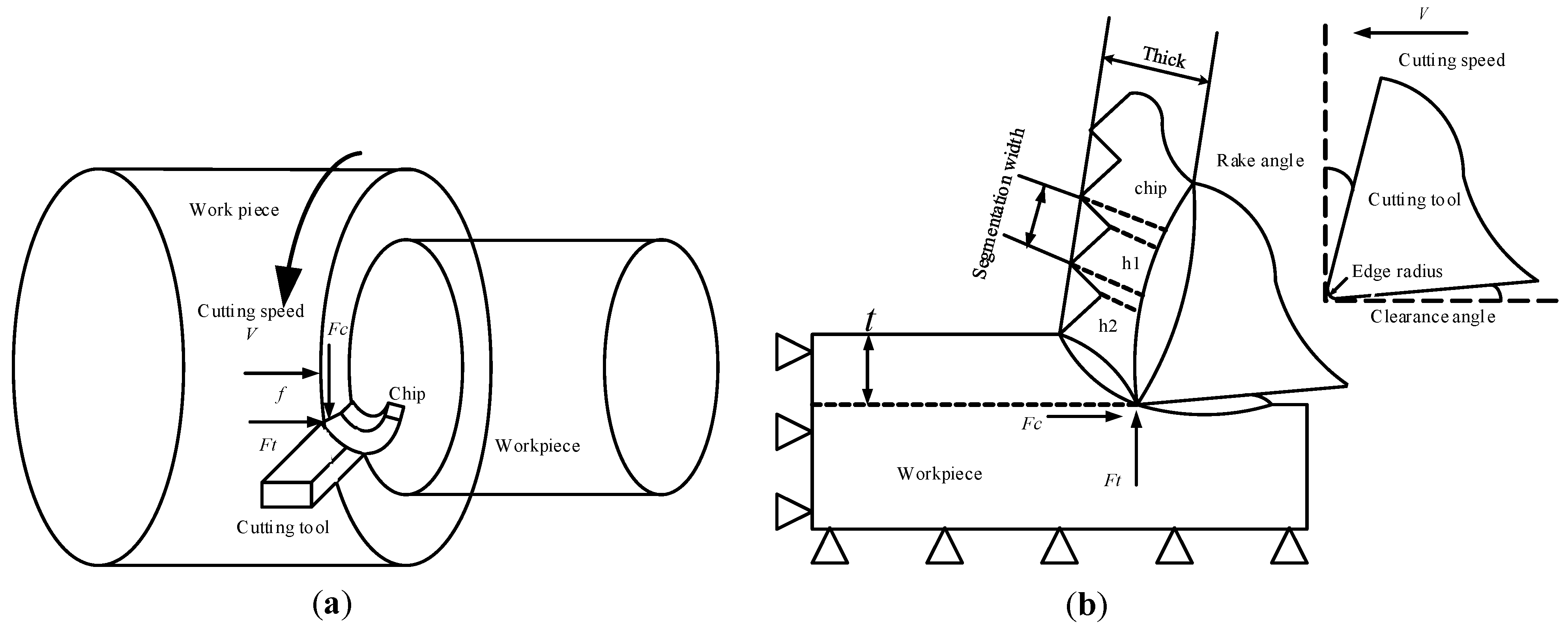
This paper gives an example of turning to show how our method works. First, a cutting model is simplified as the orthogonal cutting model. Then a numerical simulation based on the SPH method is applied to simulate the cutting process as an alternative to the real cutting experiment. Furthermore, the surface roughness of this simulation model is calculated and the variation trend of surface roughness with different cutting parameters is evaluated. After that, we employ the Taguchi method which involves establishing an orthogonal simulation array, applying an S/N ratio and ANOVA to investigate the effects of cutting parameters on surface roughness. Finally, we compare our result with experiments and make evaluations.

There are two key components in our work. The first one is to establish a reliable and accurate numerical cutting model, and the second one is to come up with a method to evaluate the variation trend of surface roughness with different cutting parameters. As for the first component, most of the traditional numerical models apply the Finite Element Method (FEM) which bears problems in handling with large deformations and material fragmentations during the cutting process and sometimes leads to simulation breakdowns caused by excessive mesh distortion [8,9,10,11]. At the same time, the simulation result is sensitive to different ways of generating the mesh, which affect the accuracy of the simulation [14]. 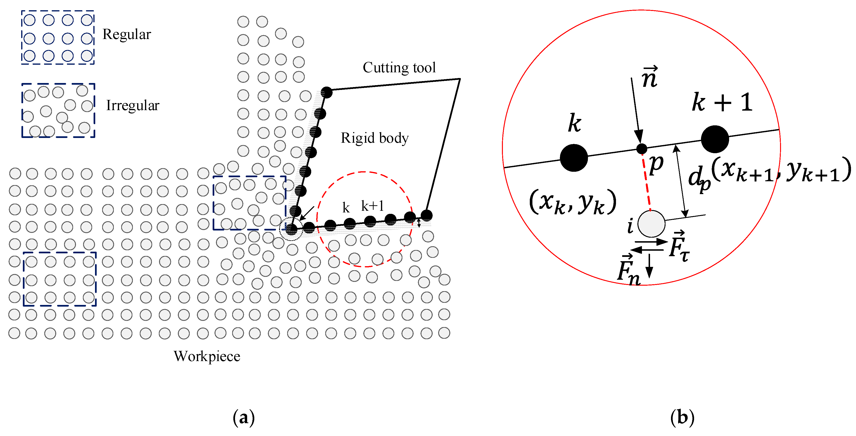Another problem of FEM is that it is not capable of deriving the surface roughness from the simulated surface since FEM simulates the cutting process, including chips formation, through setting chip separation criteria and deleting elements [9]. To avoid these problems, we applied Smoothed Particles Hydrodynamic (SPH) method, a Lagrangian meshfree method, to establish the numerical cutting model.

SPH divides material into individual particles with independent properties, such as density, mass and speed, in the process of simulation instead of generating mesh for materials and cutting tools. Compared with FEM, its adaptivity can be obtained at the early stage of approximation of field variables, and its formula is not affected by the distribution of particles. Thus, SPH is capable of handling large deformation, which always occurs during the cutting process, and at the same time, naturally simulates the process of chip separation. Previous studies have proven that SPH can simulate cutting processes effectively [8,9,10,11,15,16]

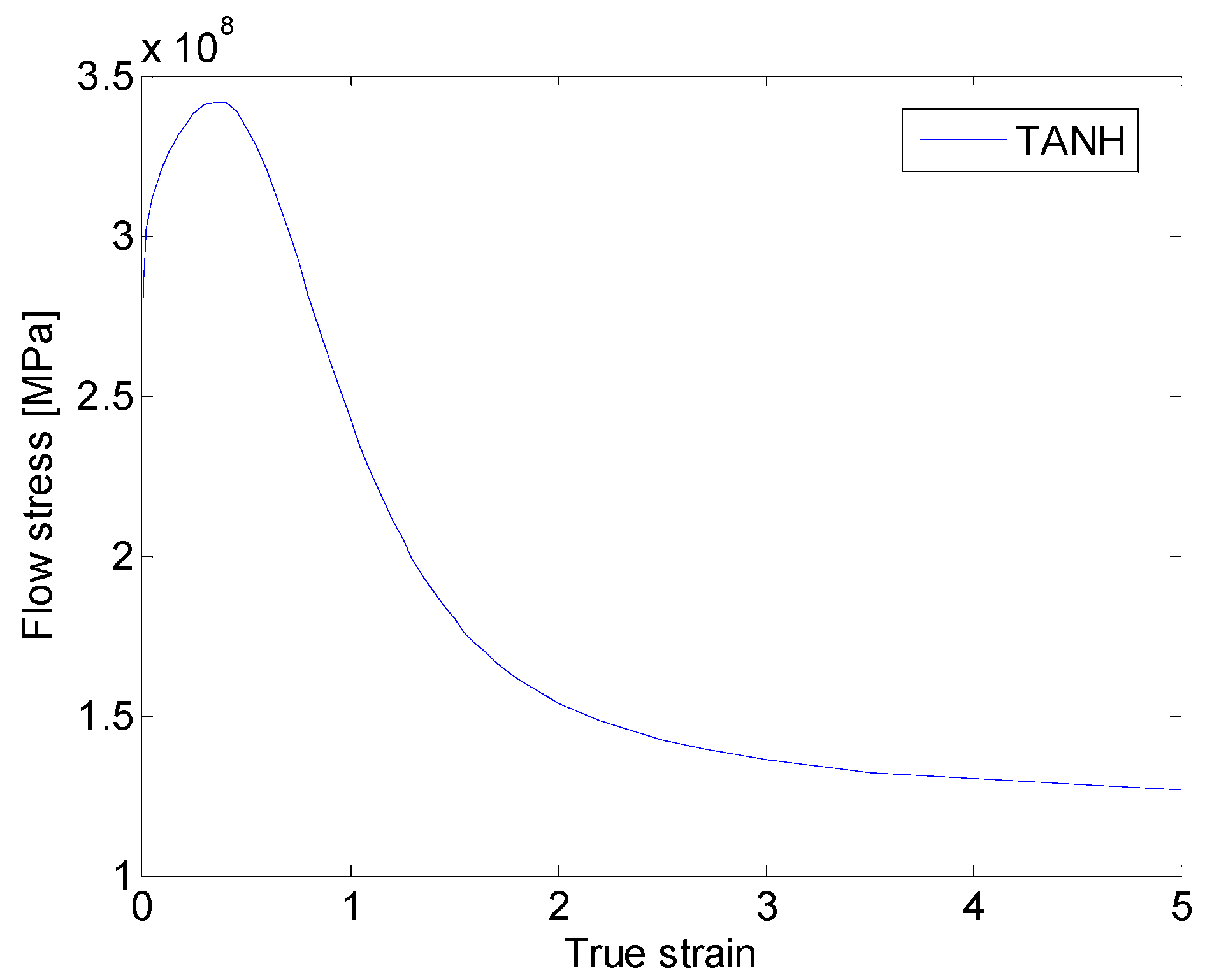
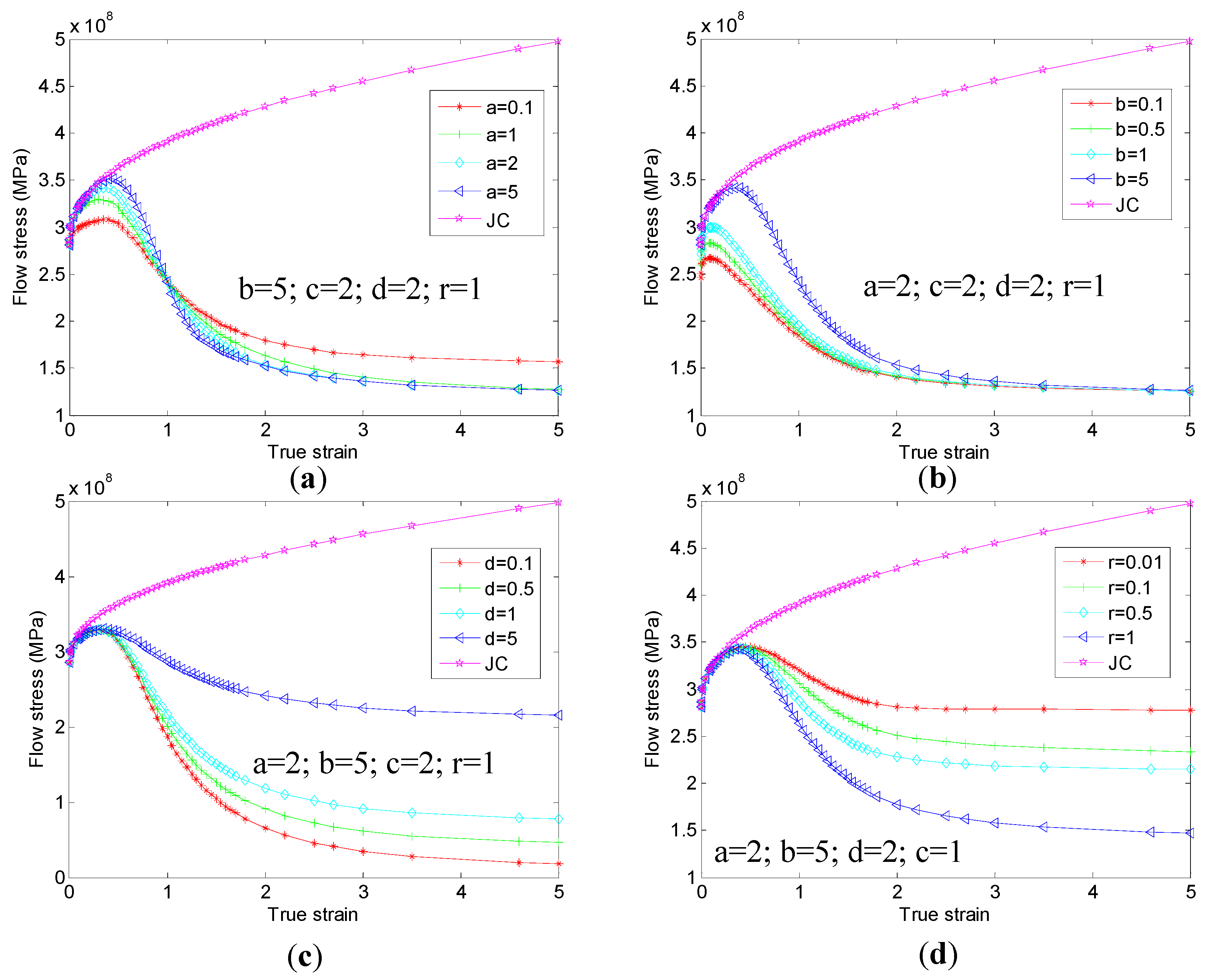
It is well known that the Johnson–Cook (JC) model [17] and Johnson–Cook damage [18,19] model are the most popular constitutive material laws in describing metal behavior. High strain and high strain rates, however, always occur in Ti–6AL–4V machining process, and under this condition, the dynamic mechanical properties of the material, such as strain softening and dynamic recrystallization mechanisms of Ti–6AL–4V materials, cannot be exactly described by JC law. This paper, hence, applies Hyperbolic Tangent (TANH) constitutive law, which was proposed by Calamaz [20] and later further developed by the Sima M and Özel T [21] to describe dynamic mechanical properties of Ti–6AL–4V material. The TANH constitutive model not only considers those problems which are mentioned above, but also describes the process of dynamic recrystallization mechanisms which also always occurs in the cutting Ti–6Al–4V process [22]. In addition, an improved SPH algorithm is adopted through adding modified schemes for approximating density (density correction) and kernel gradient approximation (kernel gradient correction) in this work, which has been proven to be very efficient in improving the accuracy of a cutting model [15]. Since the traditional SPH cannot exactly reproduce linear functions in the entire problem domain, in its initial form particle summation formulation, the SPH does not exactly reproduce a constant near the boundary because of the loss of symmetry in the smoothing operation.

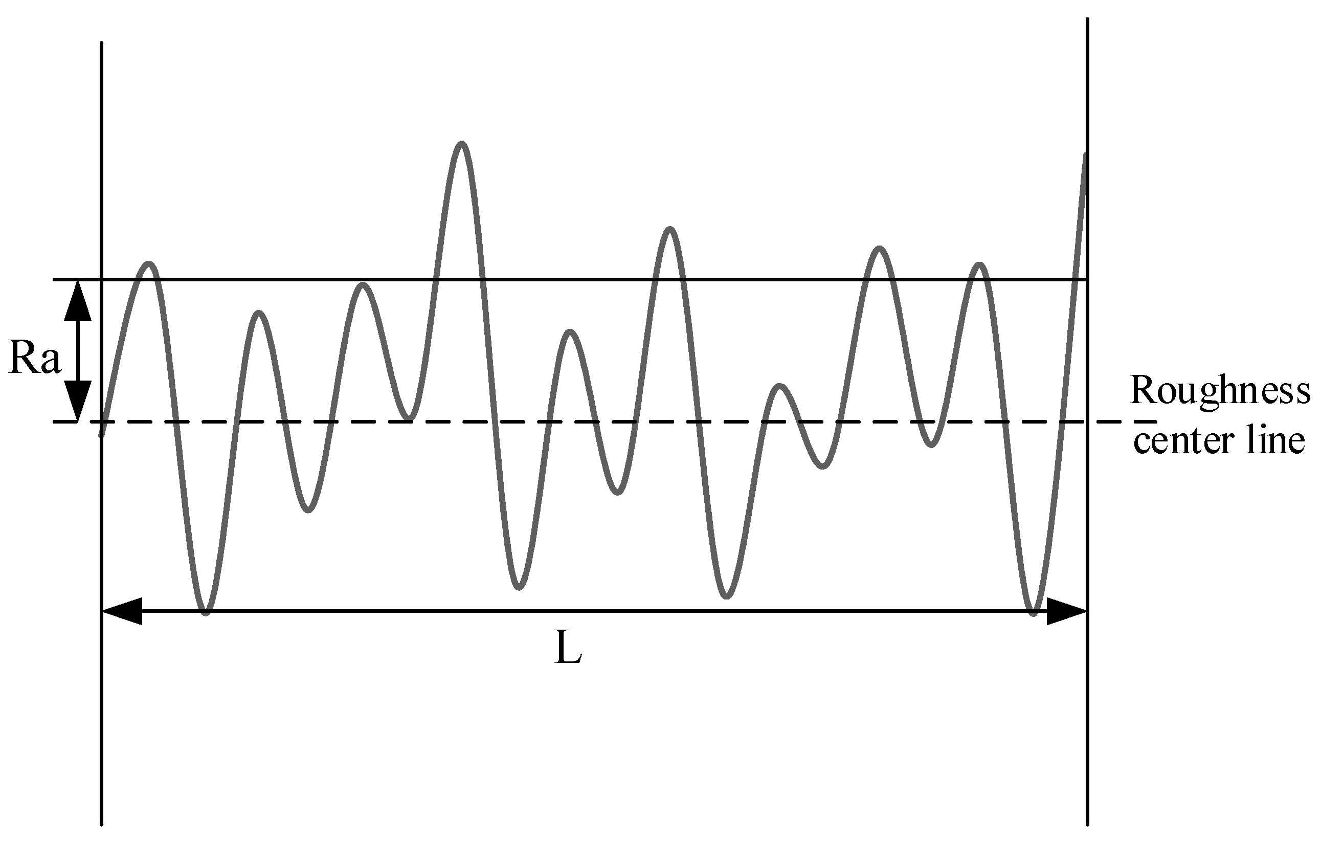
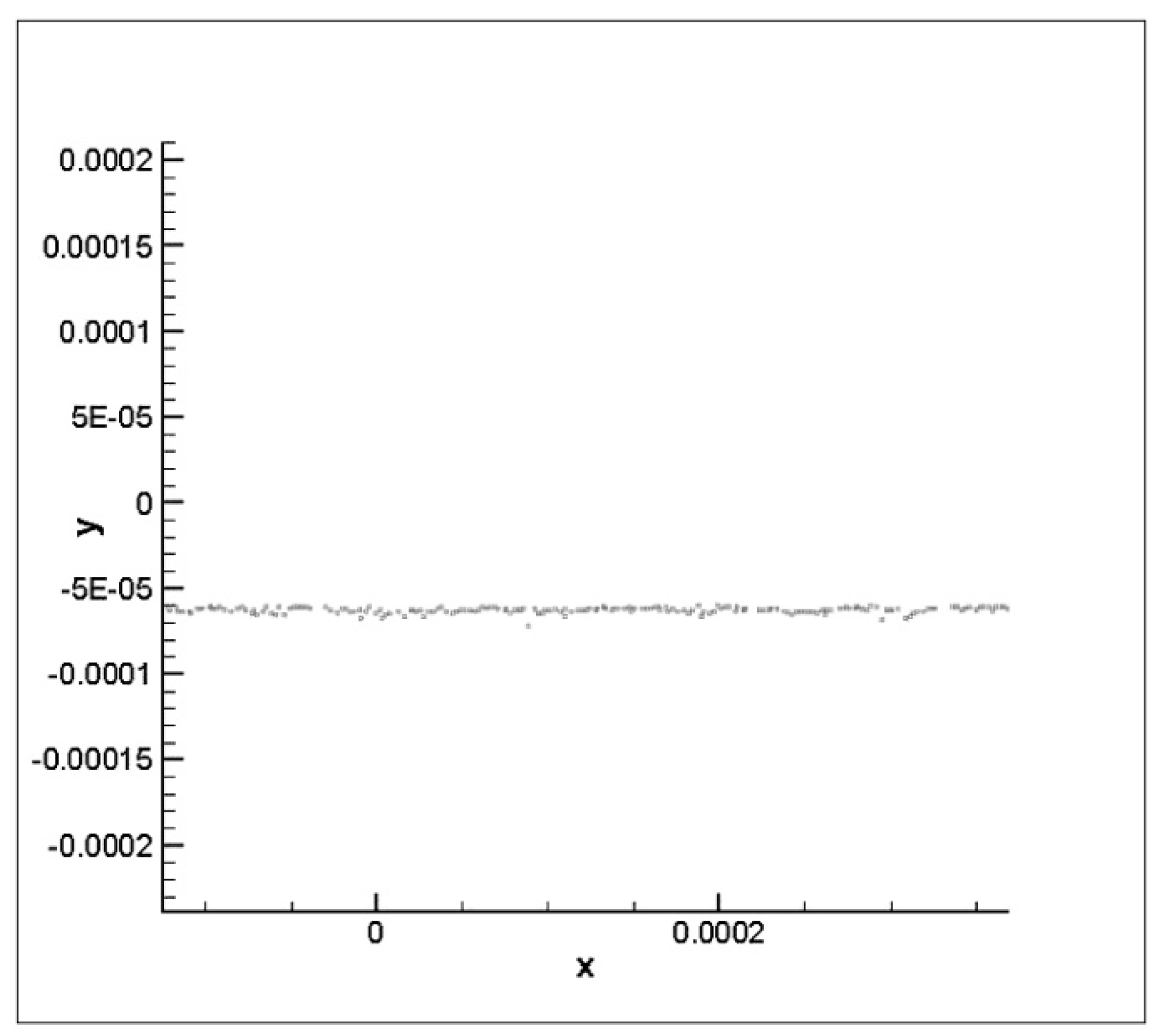
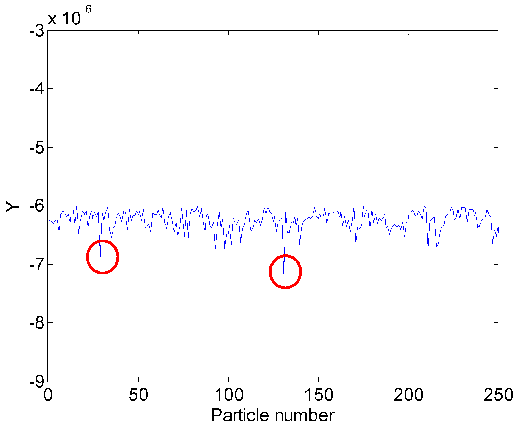
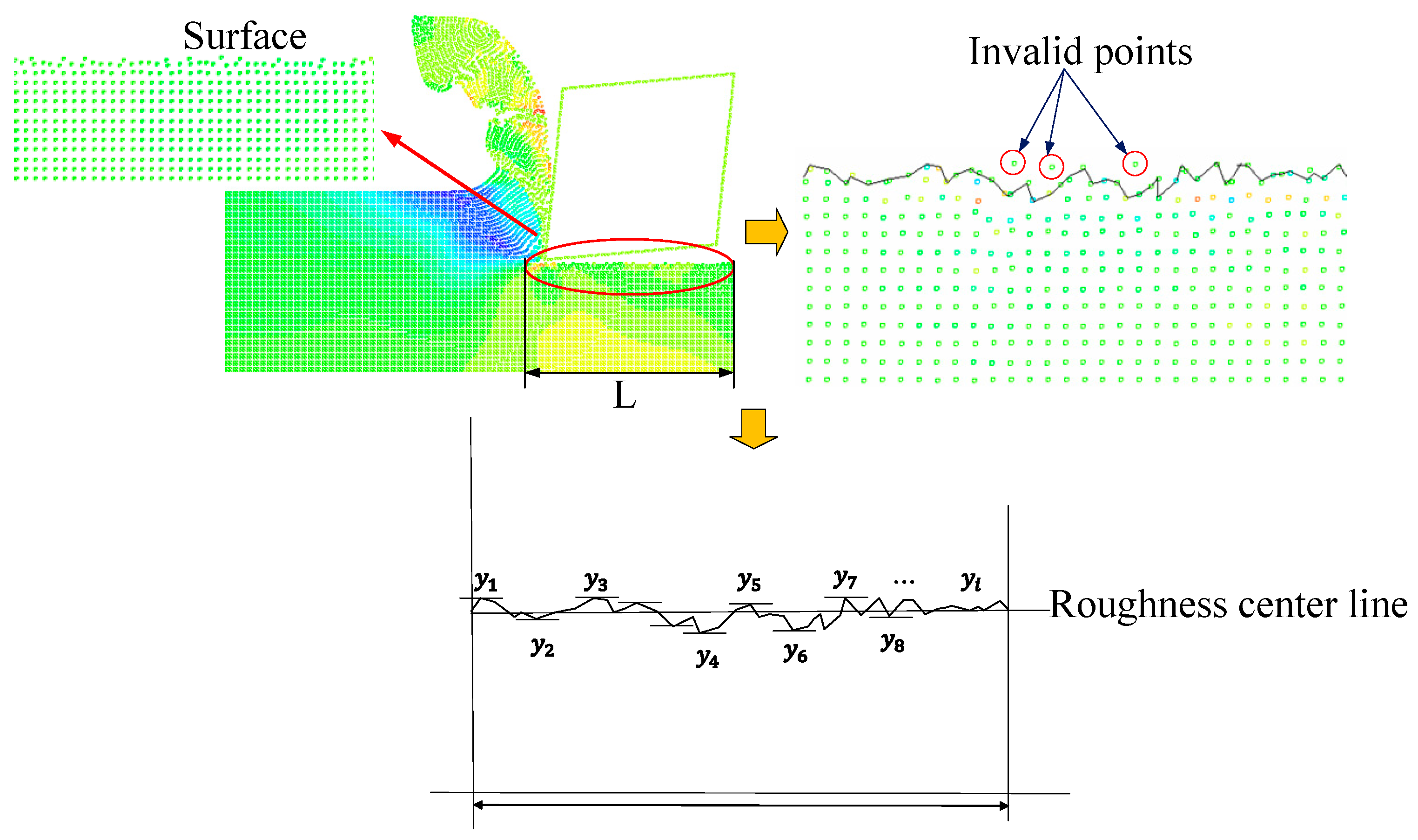
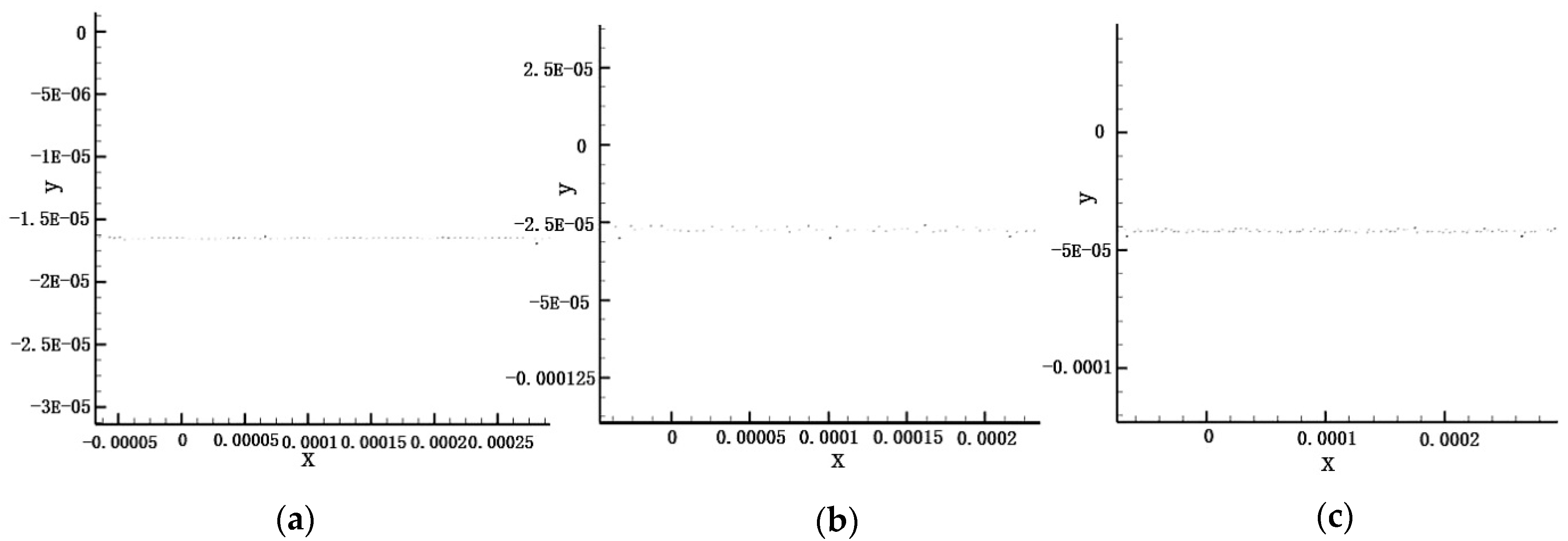
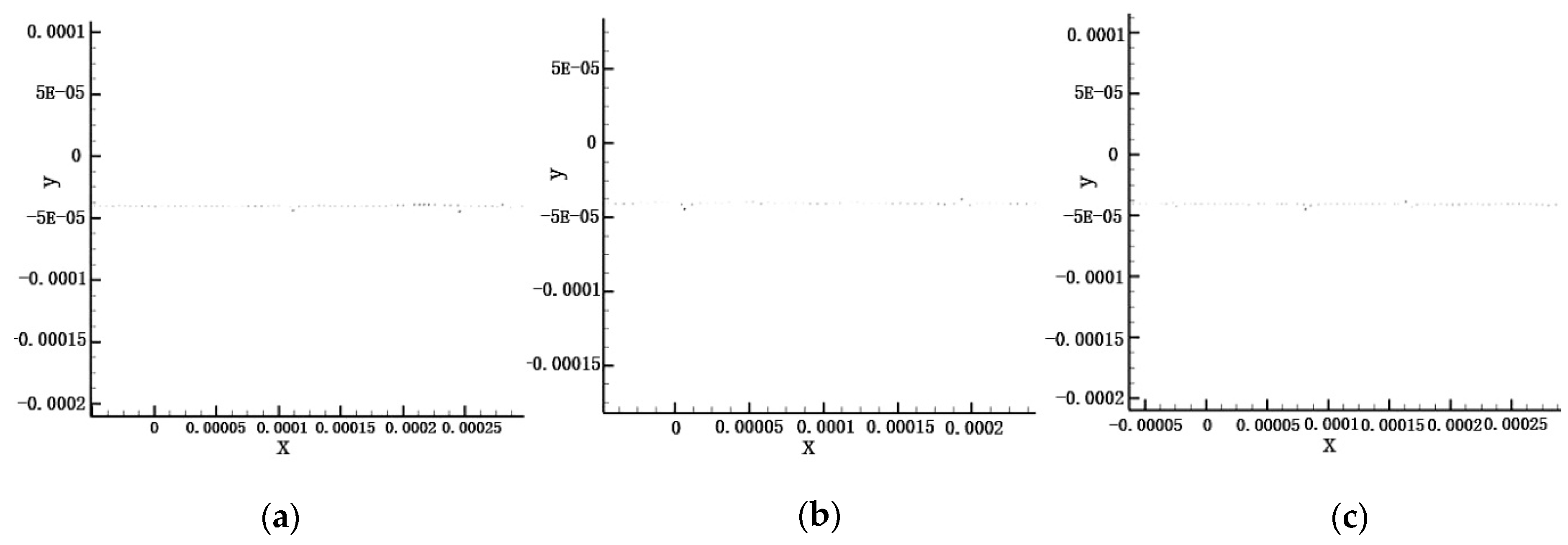
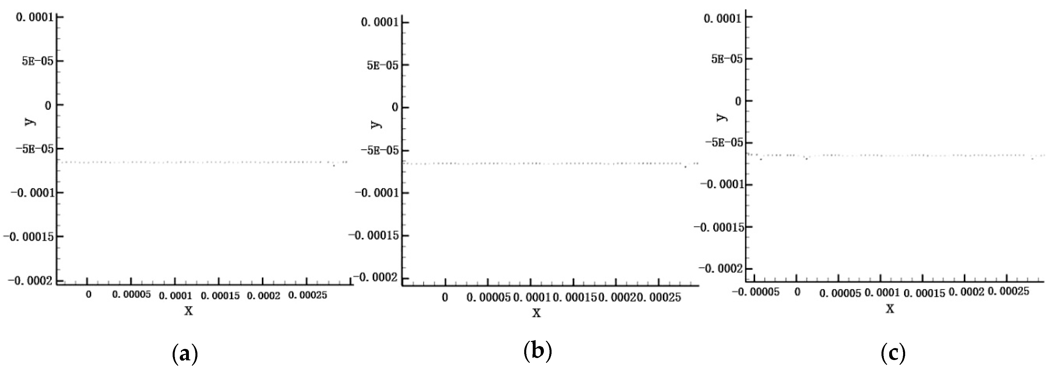
The second component involves the evaluation of the variation trend of surface roughness with different cutting parameters. The SPH algorithm adopted in this paper naturally simulates the separation of chips from the workpiece. Each individual particle carries independent attributes, such as density, mass, speed, and location. After examining the location of each individual particle of the workpiece surface and incorporating it into the definition and calculation of surface roughness, this paper proposes a method, Surface Particles Method (SPM), to calculate the surface roughness of the SPH model. Then we evaluate the variation trend of surface roughness based on the surface roughness of the SPH cutting model by changing the cutting parameters during the simulation of the cutting process.

To summarize, this paper (1) adopts an improved SPH algorithm and the TANH constitutive law to establish an improved SPH cutting model and make the simulation cutting model more accurate; (2) proposes a Surface Particles Method (SPM) to evaluate the variation trend of surface roughness with different parameters instead of the real experiments for cutting Ti–6AL–4V and substantially reduces work time and cost; (3) investigates the influence of cutting parameters on surface roughness during cutting by the Taguchi method and avoids the laborious experimental process; and 4) finally, compares our simulation results with experimental results to testify the effectiveness. The comparison shows that our method is reliable and effective to investigate the effects of cutting parameters on surface roughness.

2. SPH Modeling of Cutting Model

2.1. SPH Basic Principles

Lucy came up with SPH method in 1977 and the original purpose of this method was to solve astrophysical problems [23,24]. It was then extensively used in many different areas, such as fluid mechanics and solid mechanics [25,26]. Previous studies have proven that SPH can solve the fluent problem effectively, such as free surface flow [27,28] and bubble rising [29,30]. The cutting problem can also be regarded as a fluent (“solid-flow”) problem, since the solid deforms drastically when the solid materials are machined by a cutting tool at high speed, and thus it can be treated as a “flow” of solid materials. Therefore, SPH should be an effective method for simulating cutting processes [11,15,31,32]. The kernel approximation and particles approximation are two very important steps in the SPH method:

2.1.1. Kernel Approximation:

$$\langle f\left({\mathit{x}}_{\mathit{i}}\right)\rangle ={\displaystyle \underset{\Omega }{\int }f\left({\mathit{x}}_{\mathit{j}}\right)W\left({\mathit{x}}_{\mathit{i}}-{\mathit{x}}_{\mathit{j}},h\right)d{\mathit{x}}_{\mathit{j}}}$$

(1)

$$\langle \nabla f\left({\mathit{x}}_{\mathit{i}}\right)\rangle =-{\displaystyle \underset{\Omega }{\int }f\left({\mathit{x}}_{\mathit{j}}\right)\nabla W\left({\mathit{x}}_{\mathit{i}}-{\mathit{x}}_{\mathit{j}},h\right)d{\mathit{x}}_{\mathit{j}}}$$

(2)

where x is a three dimension coordinate vector; x_i and x_j are the positions of particles i and j; f is the function of x; f(x_j) is the value of f(x) at particle j; and Kernel function W represent a weighted contribution of particle j to particle i. The gradient of kernel function $\nabla W$ can be expressed as $\nabla W=\frac{{\mathit{x}}_{\mathit{i}}-{\mathit{x}}_{\mathit{j}}}{{\mathit{r}}_{ij}}\frac{\partial W}{\partial r_{ij}}$. h is the smooth length, which is used to define the influence domain of the smooth kernel function. In this work, we choose the cubic spline function [33], which closely resembles a Gaussian function [25], as our smoothing function. It is expressed as following:

$$W_{ij}={\alpha }_d\{\begin{array}{l}\frac{2}{3}-q^2+\frac{1}{2}{q}^3,0\le q\le 1\\ \frac{1}{6}{\left(2-q\right)}^3,1\le q\le 2\end{array}$$

(3)

where ${\alpha }_d$ is the normalization factor that can be expressed as ${\alpha }_d=15/\left(7\pi h^2\right)$. It is always used to solve 2D problems. q is the normalized distance between particle $i$ and $j$, which can be expressed as $q=r_{ij}/h$. The value of the smoothing length is chosen based on actual problems, which means the larger value may affect the computational efficiency, while the smaller value may cause low accuracy of computation. In this study, we choose the 1.5 times particle spacing as the smoothing length [15].

2.1.2. Particle Approximation

In the SPH algorithm, the computation domain can be discretized with a set of particles by using $\Delta V_j$ instead of the dx_i in Equations (1) and (2):

$$\Delta V_j=\frac{m_j}{{\rho }_j}$$

(4)

where m_j is the mass of particle j. ${\rho }_j$ is the density of particle j. N is the total number of particles which are involved in the computational field. Substituting Equation (4) into Equation (1) and Equation (2):

$$\langle f\left({\mathit{x}}_{\mathit{i}}\right)\rangle ={\displaystyle \sum }_{j=1}^N\frac{m_j}{{\rho }_j}f\left({\mathit{x}}_{\mathit{j}}\right)W\left({\mathit{x}}_{\mathit{i}}-{\mathit{x}}_{\mathit{j}},h\right)$$

(5)

$$\langle \nabla f\left({\mathit{x}}_{\mathit{i}}\right)\rangle =-{\displaystyle \sum }_{j=1}^N\frac{m_j}{{\rho }_j}f\left({\mathit{x}}_{\mathit{j}}\right)\nabla W\left({\mathit{x}}_{\mathit{i}}-{\mathit{x}}_{\mathit{j}},h\right)$$

(6)

From above, it should be noticed that some macroscopic variables (temperature, pressure, density, etc.) are expressed as integral form by a set of disorderly point values in the SPH method. In this set of points, the interaction between various points are described and a kernel estimate of a point is obtained by an interpolation function.

In the SPH equation, the governing equation is the Lagrangian form of Navier–Stokes(NS) equations [14], which is used for governing the materials. The mass conservation law and momentum conservation laws can be expressed as following:

$$\frac{d\rho }{dt}=-\rho \frac{\partial v^{\alpha }}{\partial x^{\alpha }}$$

(7)

$$\frac{d{v}^{\alpha }}{dt}=\frac{1}{\rho }\frac{\partial {\sigma }^{\alpha \beta }}{\partial x^{\beta }}+f^{\alpha }$$

(8)

where v is the velocity; t is the time; the coordinate direction can be denoted by $\alpha$ and $\beta$; $f^{\alpha }$ is the component of acceleration; and ${\sigma }^{\alpha \beta }$ is the total stress tensor which consists of two parts:

$${\sigma }^{\alpha \beta }=-P{\delta }^{\alpha \beta }+{\tau }^{\alpha \beta }$$

(9)

where P is pressure; ${\delta }^{\alpha \beta }$ is the Kronecker tensor; and ${\tau }^{\alpha \beta }$ is the deviatoric shear stress.

The shear stresses are generated and change with time when solids are in the dynamic velocity field with spatial gradients. The stress $\tau$ can be expressed as following [14]:

$$\frac{d{\tau }_i{}^{\alpha \beta }}{dt}=2G({\dot{\epsilon }}_i^{\alpha \beta }-\frac{1}{3}{\delta }^{\alpha \beta }{\dot{\epsilon }}_i^{\gamma \gamma })+{\tau }_i{}^{\alpha \gamma }\cdot {\dot{r}}_i^{\beta \gamma }+{\tau }_i{}^{\gamma \beta }\cdot {\dot{r}}_i^{\alpha \gamma }$$

(10)

where ${\dot{\epsilon }}^{\alpha \beta }$ is the strain rate tensor; $G$ is the shear modulus which can be obtained by an experimental test; and ${\dot{r}}^{\alpha \beta }$ is the rotation tensor. After elastic deformation, the material will enter the plastic deformation named plastic behavior and it can be identified by the critical point of plastic deformation [14]:

$$f_y=\frac{{\sigma }_y}{\sqrt{3J_2}}$$

(11)

where J₂ is the second stress tensor invariant. ${\sigma }_y$ is the flow stress and its initial value is the shear stress (${\sigma }_y=\sqrt{{\tau }^{\alpha \beta }·{\tau }^{\alpha \beta }}$). When the value of $f_y$ is lower than 1 ($f_y<1$), the plastic deformation is said to occur.

As mentioned above, the traditional SPH method has low accuracy [34]. Therefore, in this study, we employed an improved SPH method where density and kernel gradient are corrected by Moving Least Squares and a correction matrix. It has been proven to be efficient in improving the accuracy of the cutting model [15].

In the scheme of the improved SPH algorithm, we use the Moving Least Squares (MLS) method to correct the density field periodically; the linear variation of the density field can be exactly reproduced and a smoother pressure can be obtained [35]. The correction scheme is expressed as:

$$\langle {\rho }_i\rangle ={\displaystyle {\sum }_j^N{\rho }_j}{W}_{ij}^{MLS}\frac{m_j}{{\rho }_j}={\displaystyle {\sum }_j^N{m}_j{W}_{ij}{}^{MLS}}$$

(12)

where $W_{ij}^{MLS}$ is the MLS kernel; more details can be found in Reference [35].

The Kernel Gradient Correction (KGC) method is applied to improve the SPH approximation accuracy. The second order accuracy of SPH approximation can also be restored by this correction scheme. The corrected value of ${\nabla }_i^{new}{W}_{ij}$ for arbitrary particle i is expressed as follows:

$${\nabla }_i{}^{new}{W}_{ij}=L{(r_i)}^{-1}{\nabla }_i{W}_{ij}$$

(13)

where $L\left(r_i\right)$ is the correct matrix, which can be expressed as:

$$L(r_i)={\displaystyle {\sum }_j\left[\begin{array}{cc}{x}_{ij}\frac{\partial W_{ij}}{\partial x_i}& y_{ji}\frac{\partial W_{ij}}{\partial x_i}\\ x_{ji}\frac{\partial W_{ij}}{\partial y_i}& y_{ji}\frac{\partial W_{ij}}{\partial y_i}\end{array}\right]}{V}_j$$

(14)

Finally, the SPH computational domain is discretized by a limited number of particles which have their own attributes such as mass (m) and individual space. The continuity equation finally is expressed as following:

$$\frac{d{\rho }_i}{dt}={\rho }_i{\displaystyle \sum _{j=1}^N\frac{m_j}{{\rho }_j}}{v}_j^{\beta }\cdot \frac{\partial W_{ij}}{\partial x_i^{\beta }}$$

(15)

The momentum equation is expressed as following:

$$\frac{d{v}_i^{\alpha }}{dt}={\displaystyle \sum _{j=1}^N{m}_j}\left[-\left(\frac{P_i+P_j}{{\rho }_i{\rho }_j}\right){\delta }^{\alpha \beta }+\frac{{\tau }_i^{\alpha \beta }+{\tau }_j^{\alpha \beta }}{{\rho }_i{\rho }_j}-{\displaystyle {\prod }_{ij}{\delta }^{\alpha \beta }}\right]\cdot \frac{\partial W_{ij}}{\partial x_i^{\beta }}+f_i^{\alpha }$$

(16)

where ${\prod }_{ij}$ is called artificial viscosity and is used to reduce the unphysical oscillations in the numerical results around the shocked region.

2.2. Material Constitutive Model

Johnson–Cook (JC) is the most frequently adapted constitutive law to describe the dynamic mechanism properties (strain hardening, strain hardening rate and thermal softening) of mental material when the elastic deformation transforms to the plastic deformation stage. The JC constitutive law, however, does not take into account the strain-softening of the material under high strain conditions. Cutting Ti–6AL–4V, however, is a high stress and high stress rate process, and JC law cannot describe this process accurately. To solve the problems of JC law, Calamaz proposed a TANH constitutive law which modifies the stress, strain and temperature components of JC law by adding a, b, c, d parameters and a tanh function [20]. Later, Sima M and Özel T introduced exponent r into the TANH constitutive model to further control the tanh function for thermal softening [21]. The TANH constitutive model not only considers the stress softening of the material as shown in Figure 1, but also considers the recrystallization phenomenon. Figure 1 is the flow stress-strain curve with the TANH law.

$${\sigma }_y=\left[A+B{(\frac{1}{\exp ({\epsilon }_{eff}^a)})}^N\right]\left[1+Cln\left(\frac{{\dot{\epsilon }}_{eff}}{{\dot{\epsilon }}_0}\right)\right]\left[1-{\left(\frac{T-T_{room}}{T_{melt}-T_{room}}\right)}^M\right](D+(1-D){(\tanh (\frac{1}{{\left(\epsilon +S\right)}^c}))}^r)$$

(17)

$$D=1-{(\frac{T}{T_m})}^d$$

(18)

$$S={\left(\frac{T}{T_m}\right)}^b$$

(19)

$$T=e/C_p+T_{room}$$

(20)

where ${\epsilon }_{eff}$ is the equivalent plastic strain; ${\dot{\epsilon }}_{eff}$ is the equivalent plastic strain rate; ${\dot{\epsilon }}_0$ is the reference plastic strain rate; A, B, C, N, and M are material-dependent constants which are the same parameters as in the JC equation and are obtained by SHPB tests [36]. $T_{room}$ is the room temperature. $T_{melt}$ is the melting temperature of Ti–6AL–4V. T is the current temperature which is computed by Equation (20). a, b, c, d and r are corrected parameters which are obtained by the control variable method. We vary one parameter while keeping the others constant to investigate the effects of the parameters on strain-stress curves and make the strain-curve of the TANH model be in good agreement with that of the JC model under the low strain (the strain can be considered low strain when the strain is lower than 0.5). As shown in Figure 2a, parameter a controls the strain-hardening part by decreasing flow stress after a critical strain value, and a low value of the parameter will lead to a big difference between TANH and the SHPB test data. As a increases, the maximum stress will increase. Parameter b in (Equation (19)) controls the temperature-dependent flow-softening effect and points out where the maximum flow stress is attained. The lower the value of parameter b is, the lower the strain value of the peak flow stress that occurs, as shown in Figure 2b. Parameter d is an exponent for the temperature that controls the degree of temperature dependency of parameter D as given in (Equation (18)). As shown in Figure 2c, parameter d has a strong impact on the value of flow softening and it determines the minimum flow stress value. As shown in Figure 2d, parameter r controls the softening trend. The higher the parameter r is, the faster the flow stress-strain curve enters the softening region. With the strain increasing, the slope of strain softening curves will decrease and the maximum flow stress remains unchanged. The c has similar effects to r on the flow stress [16]. After observing the trend of the curve with different parameters, the best fit parameters and best stress-strain curve are given in

Table 1. Material properties of Ti–6AL–4V for workpiece [36,37].

Physical Parameter	Constant	Work Material (Ti–6AL–4V)
Density, ρ0 (Kg/m3)		4430
Possion’s ratio v		0.342
Shear modulus (G)		110 Gpa
Specific heat, Cp J/(Kg·K)		580
Thermal conductivity (W/mk)		7.3
Tmelt (°C)		1878
Troom (°C)		25
TANH model (Equation (17))	A	968 $\mathrm{Mpa}$
	B	380 $\mathrm{Mpa}$
	C	0.02
	N	0.577
	M	0.421
	a	0.05
	b	2
	c	1
	d	1
	r	5

and Figure 1.

2.3. Contact Algorithms

Figure 3a provides a conceptual explanation of the particle distribution and interaction and how the contact algorithm is used to calculate the contact force. In this work, the total number of particles is 25,000 and the time step is 3.0^-9 s. (When the number of particles is greater than 25,000 or the time step is less than 3.0^-9 s. The accuracy of the model does not change obviously, while the running time of the program will increase with the increase of particles and decrease of time step). The cutting tool and material are regarded as groups of particles in our improved SPH cutting model. We treat the cutting tool as a rigid body without carrying any attributes as the workpiece material, such as density and quality. The location information $\left(x_k,y_k\right)$ and velocity information $\left(u_k,v_k\right)$ are only needed to set up for the particles of the cutting tool, which is computed by the initial location and velocity of the cutting tool respectively. Then, this information is used to calculate surface vectors (unit tangent vector and unit normal vector). We can use them to determine the direction of the cutting force and contact location between the cutter and workpiece respectively. When the cutter contacts the workpiece, two different kinds of particles (i.e. particles of the workpiece and particles of the cutter) occur contact force. To acquire the contact force, we need to 1) set a threshold $d_0$ to decide when the contact is considered to occur, and 2) calculate the contact force.

Figure 3b illustrates how the cutting tool and workpiece are regarded as the contact. P is the vertical point from particle i to the surface of the cutting tool. $d_p$ is the actual vertical distance between particle i and the cutting tool. $d_0$ is the contact threshold for these two kinds of particles. When $d_p$ is smaller than $d_0$, these two particles contact. The tangent vector ${\mathit{\tau }}_{\mathit{p}}$ and normal vector ${\mathit{n}}_{\mathit{p}}$ at point $\mathit{p}$ are calculated by the following Equation:

$$\{\begin{array}{c}{\mathit{\tau }}_{\mathit{p}}=\left(t_x,t_y\right)=\left(\frac{x_{k+1}-x_k}{\left|{\mathit{x}}_{\mathit{k}+1}-{\mathit{x}}_{\mathit{k}}\right|},\frac{y_{k+1}-y_k}{\left|{\mathit{x}}_{\mathit{k}+1}-{\mathit{x}}_{\mathit{k}}\right|}\right)\\ {\mathit{n}}_p=\left(-t_y,t_x\right)=\left(-\frac{y_{k+1}-y_k}{\left|{\mathit{x}}_{\mathit{k}+1}-{\mathit{x}}_{\mathit{k}}\right|},\frac{x_{k+1}-x_k}{\left|{\mathit{x}}_{\mathit{k}+1}-{\mathit{x}}_{\mathit{k}}\right|}\right)\end{array}$$

(21)

where x_k+1 and x_k are the coordinate values of cutting tool particle k and k + 1.

The next step is to calculate the contact force between the particles of the workpiece and cutting tool. The forces on point i have two parts, the force along the normal direction and the force along the tangential direction. The forces are calculated as the following Equation:

$$\{\begin{array}{c}{\mathit{F}}_{\mathit{n}\mathit{i}}=\left[\frac{m_i}{{\left(\Delta t\right)}^2}\left(d_0-d_p\right)\right]\cdot {\mathit{n}}_{\mathit{p}}\\ {\mathit{F}}_{\mathit{\tau }\mathit{i}}=min\left\{\left(\frac{\mu {\mathit{F}}_{\mathit{\tau }\mathit{i}}}{\left|{\mathit{F}}_{\mathit{\tau }\mathit{i}}\right|}\left|{\mathit{F}}_{ni}\right|\right),\frac{m_i}{\Delta t}\left({\mathit{v}}_{\mathit{p}\mathit{i}}\cdot {\mathit{\tau }}_{\mathit{p}}\right)\cdot {\mathit{\tau }}_{\mathit{p}}\right\}\end{array}$$

(22)

where $m_i$ is the mass of particle $i$; ${\mathit{v}}_{\mathit{p}\mathit{i}}={\mathit{v}}_{\mathit{p}}-{\mathit{v}}_{\mathit{i}}$, ${\mathit{v}}_{\mathit{p}}$ is the velocity at point $\mathit{p}$. ${\mathit{v}}_{\mathit{i}}$ is the velocity of particle i. $\mu =0.3$ is the friction coefficient between the workpiece and cutting tool [15,35]. According to the formulas above, the interaction forces between the cutting tool and workpiece are calculated [15].

3. OptimalC parameters

3.1. Evaluation of the Surface Roughness of the SPH Cutting Model

The surface roughness is the repeating series of peaks and valleys on the surface. It is calculated as the average deviation from the ideal along the direction of the normal vector of the real surface. Figure 4 illustrates the surface profile of a workpiece sample. The x axis is regarded as the central line. In the real measurement, the surface of the workpiece is discretized into measurement points. The vertical distance from the point to the center line is measured, and then the average value of these vertical distances is calculated as surface roughness R_a. The more measurement points there are, the more accurate R_a is. The equation is expressed as:

$$R_a=\frac{1}{N}{\displaystyle {\sum }_i^N\left|y(x_i)\right|}$$

(23)

N is the number of sampling points.

Similar to calculating the surface roughness derived from the vertical distances of measurement points, we extract particles on the simulated surface from the improved SPH cutting model and transform their location information into a coordinate (The SPH cutting model is established in the coordinate system and each particle has the corresponding particle number and coordinate position information. When the surface particles are extracted, the particle number of surface particles are obtained as well as the coordinate information of the particles). Figure 5 demonstrates the particles of the simulated surface after cutting, and Figure 6 illustrates the surface profile of the extracted particles under a coordinate system. We extract the coordinate information of these particles and calculate the surface roughness.

Based on the coordinate, we calculate the vertical distance from each particle to the center line. In Figure 4, the y coordinate value of the center line is the difference between workpiece height and cutting depth.

$$f_{\begin{array}{l}centerline\\ \end{array}}=H-h$$

(24)

where H is the high value of the workpiece and h is the cutting depth. What is worth noting is, since there is a small amount of random errors in the simulating process, a tiny number of particles deviate far from the center line, which does not conform to the real cutting process (When the distance between a surface particle and the roughness center line is greater than 0.5 µm, we consider this particle deviate far from the center line). Thus, we regard these particles as outliers and remove them when calculating surface roughness. Figure 7 is the steps of surface roughness calculation.

Figure 8, Figure 9 and Figure 10 show the distribution of surface particles extracted from the cutting model under different cutting parameters. These figures show that while the higher feed and smaller rake angle lead to a more disordered distribution of the surface particles (i.e., the more rough surface), the cutting speed does not exert a significant effect on the surface roughness since the order of particles did not change too much compared to the other two cutting parameters when cutting speed was changed.

3.2. The Basic Principle of Taguchi Method

Taguchi proposed a method [38] which considers the improvement of product quality. The product quality can be obtained by designing rather than inspecting. In this study, we employed the Taguchi method to investigate the effects of cutting parameters on surface roughness. The Taguchi method has two core analysis tools. The first core is the orthogonal array. Since the orthogonal array can ensure the impartiality and uniformity of the experiment’s data, it is very representative and can comprehensively reflect the impact of various factors and each level on indicators. Therefore, compared to the traditional experimental design which has a large number of experiments and is too complex, the orthogonal array can simplify the complex experimental tests and minimize the effects of the factors which are out of control otherwise. The second core is the signal-to-noise expecting (ined by design rather than the (S/N). The S/N ratio is calculated based on the experimental results of the orthogonal array, which can indicate the loss of product quality [39]. Usually, there are three performance characteristics in analyzing the S/N ratio. They are the smaller-the-better characteristic, the nominal-the-better characteristic and the larger-the-better characteristic. Neglecting the grouping of the above performance characteristic, the greatest S/N value stands for the best performance characteristic. Hence, the higher the S/N ratio is, the better the level of the cutting parameters is. In addition, the variance analysis (ANOVA) is applied to determine which cutting parameters have a significant effect. By analyzing the S/N ratio and variance, we can not only investigate the effects of cutting parameters, but also obtain the optimal cutting parameters. It should be noticed that we need to obtain the cutting parameters which achieve the lowest surface roughness value. The performance characteristic in analyzing the S/N ratio is the smaller-the better. The equations are as following:

$$M.S.D=\frac{1}{n}{\displaystyle \sum _{i=1}^n{y}_i^2}$$

(25)

$$S/N=-10\log (M.S.D)$$

(26)

where M.S.D is the mean-square deviation; n is the total number of experiments; y_i is the measured value of surface roughness; and i is the serial number of the experiment.

In this paper, the turning process (Figure 11a) is approximated as the orthogonal cutting process [40] (Figure 11b). The parameters in turning can be approximated by the orthogonal cutting parameters as shown in

Table 2. Approximation of Turning by Orthogonal Cutting [40].

Turning Operation	Orthogonal Cutting
Feed f=	Chip thickness before cut t
Cutting speed V=	Cutting speed V
Rake angle γ=	Rake angle γ
Clearance angle β=	Clearance angle β
Cutting force Fc=	Cutting force Fc
Feed force Ft=	Feed force Ft

.

As shown above, the three parameters (cutting speed, feed and rake angle) can be controlled by this simulating cutting model. They can also affect surface roughness significantly in the actual turning process. Therefore, the reasonable choice of them would improve the surface quality and decrease the surface roughness. Though the cutting depth and clearance angle in turning are other parameters in the cutting process, the cutting depth cannot be controlled in the 2D simulation model and clearance angle has little effect on surface roughness. In this work, we only consider the above three factors on surface roughness and therefore we choose them as controllable factors in this work. In addition, three levels are also considered in this experiment, as shown in

Table 3. Three levels for cutting parameters.

Symbol	Cutting Parameters	Level1	Level2	Level3
A	Rake angle	0°	3°	7°
B	Cutting speed	240 m/s	120 m/s	60 m/s
C	Feed	0.07 mm	0.1 mm	0.13 mm

. Therefore, as shown in

Table 4. L₉ orthogonal array in simulated experiments.

Experiment Number	Cutting Parameter Level
	A	B	C
	Rake Angle	Cutting Speed	Feed
1	1	1	1
2	1	2	2
3	1	3	3
4	2	1	3
5	2	2	1
6	2	3	2
7	3	1	2
8	3	2	3
9	3	3	1

, we selected L₉ orthogonal array as our experimental design [41]. It should be noticed that to select an appropriate orthogonal array for the experiments, the total degree of freedom needs to be computed. The degrees of freedom are defined as the number of comparisons between the process parameters that need to be made to determine which level is better and specifically how much better it is. In this study, the L₉ array which has four columns and nine rows has eight degrees of freedom and it can handle three-level process parameters (There are six degrees of freedom owing to there being three cutting parameters in the turning operations).

To summarize, we use L₉ orthogonal array to design the simulated experiment, and then we study the influence of different cutting parameters (cutting speed, feed and rake angle) on surface roughness by analyzing the S/N ratio and variance. Based on these results, we obtain the effects of cutting parameters on surface roughness and optimize the cutting parameters to achieve the lowest surface roughness [41,42].

4. Results and Discussion

4.1. Experiment Test for Improved SPH Cutting Model

We established an improved SPH cutting model which incorporated the improved SPH algorithm, TANH constitutive model and contact algorithm. The improved cutting model is validated by comparing results from Calamaz et al [37]. The following Figure 12 is the comparison between the simulated cutting process and the experiment (chips morphology formation is recorded by a camera in the experimental cutting process) both under the same cutting parameters (cutting depth, 0.1 mm; cutting speed, 235 m/min; and edge radius, 20 μm, rank angle 0°, clearance angle 11°). It shows that the simulation results, such as strain localization along a curved shear and the curvature change of a slipped shear band (new segment), match the experiments very well.

In addition, the accuracy of the cutting model can be verified by the segmented chip morphology and cutting force. We can compare three parameters of chip morphology between the simulation and experiments, such as segmentation width (W), maximum segmentation height (h1) and minimum segmentation height (h2), as shown in Figure 12. The comparisons of simulation and experimental chip morphology are presented in Figure 13, Figure 14 and Figure 15.

Table 5. Comparison of errors in the simulation and experimental data for segmentation characteristics.

Speed	h1 (Relative Error %)	h2 (Relative Error %)	W (Relative Error %)
75	9.84%	8.70%	5.19%
94	8.96%	−6.85%	2.41%
116	−19.35%	−13.48%	4.94%
150	2.80%	−2.35%	14.29%
188	13.14%	−8.45%	5.06%
233	12.90%	10.45%	11.11%

shows the comparison of relative error in simulation and experimental data for segmentation characteristics.

The average cutting force and average thrust force are predicted under different cutting speeds by the improved SPH model. Figure 16 and Figure 17 show the comparison between the simulated results and the experimental results [37].

Table 6. Comparison of errors in the simulation and experimental data for cutting force and feed force values.

Speed	Cutting Force (Relative Error %)	Thrust Force (Relative Error %)
75	−7.49%	−11.03%
94	−3.87%	16.34%
116	−7.24%	−11.39%
150	−10.26%	9.42%
188	−8.67%	−7.83%
233	−7.73%	8.64%

compares the quantitative differences in relative errors between the simulation and experimental results for cutting force and thrust force.

Regarding the verification of the model, the h1, h2, and segment width and forces have been proven to be effective and efficient factors for verifying cutting models [15,19,20,37]. From the comparison of the simulation and the experiment in terms of segmentation width, maximum segmentation height (h1) and minimum segmentation height (h2), cutting force and thrust force, we can conclude the improved SPH cutting model simulates the cutting process accurately and effectively.

4.2. Analysis of the S/N Ratio and Variance

The surface particles are extracted and the coordinates of particles are obtained to calculate the surface roughness of the simulation model.

Table 7. Simulation results for surface roughness and S/N ratio.

Experiment Number	Cutting Parameter Level			Model Surface Roughness (10−1 µm)	S/N Ratios for Surface Roughness
	A	B	C
	Rake Angle	Cutting Speed	Feed
1	0°	240 m/s	0.07 mm/rev	2.251	−7.048
2	0°	120 m/s	0.1 mm/rev	6.136	−15.758
3	0°	60 m/s	0.13 mm/rev	12.256	−21.767
4	3°	240 m/s	0.13 mm/rev	3.191	−10.079
5	3°	120 m/s	0.07 mm/rev	5.341	−14.553
6	3°	60 m/s	0.1 mm/rev	2.086	−6.387
7	7°	240 m/s	0.1 mm/rev	2.693	−8.605
8	7°	120 m/s	0.13 mm/rev	1.020	−0.172
9	7°	60 m/s	0.07 mm/rev	1.753	−4.876

shows the simulation results of the surface roughness value and S/N ratio for surface roughness.

Table 8. S/N ratio response table.

Symbol	Cutting Parameter	Mean S/N Ratio
		Level 1	Level 2	Level 3	Max-min
A	Rake angle	−14.8574	−8.5769	−4.5353	10.3221
B	Cutting speed	−9.3391	−10.1607	−10.2373	0.8982
C	Feed	−4.5508	−11.0096	−14.9747	10.4239

Total mean S/N ratio = −9.8046.

is the S/N response table for surface roughness; it gives each level a mean S/N ratio and the total mean S/N ratio. In addition, the different values of the S/N ratio between maximum and minimum are also given in Table 8. It can be seen that the feed and rake angle have the highest difference value, 10.3221 and 10.4239 respectively. According to the Taguchi method, the larger the difference between the values of the S/N ratio are, the more effect there will be on surface roughness. Therefore, changing the feed and rake angle will change the value of surface roughness of the simulation model significantly.

Figure 18 shows the S/N response graph for surface roughness. As mentioned in Equation (25) and Equation (26), a greater value of the S/N ratio will have a smaller variance of surface roughness (the smaller the better).

The variance analysis (ANOVA) is also a helpful and efficient tool for testing and determining which cutting parameter have an obvious effect on surface roughness. As shown in

Table 9. Variance analysis for surface roughness.

Parameters	Degree of Freedom	Sum of Squares	Mean Square	F Ratio	Contribution (%)
Rake angle	2	160.15	80.073	28.493	45.602
Cutting speed	2	9.1471	4.5736	1.6275	1.0407
Feed	2	163.94	81.969	29.168	46.721
Error	2	5.6202	2.8101		6.6345
Total	8	338.85			100

, it shows the rake angle and feed have an obvious effect on the surface roughness, while the cutting speed compared to other parameters has little effect on surface roughness, since their contributions in percentage are 45.602, 46.721 and 1.0407 respectively. In addition, if we only consider these three parameters for lowering the surface roughness in cutting processing. The best of combinations of the cutting parameters (the level 3 of rake angle, the level 1 of cutting speed, and the level 1 of feed) can be obtained according to analyze the S/N ratio and variance.

4.3. Experimental Tests for Effect of Cutting Parameters on Surface Roughness

We apply the turning (dry cutting) and single-point cutting as our experimental test. Figure 19 shows the experimental instruments. The cutting tool used carbide inserts and a tool holder. We applied three different carbide inserts and a different tool holder. These inserts have the same nose radius 0.8 mm and edge radius 20 μm. After installation, the effective rake which is a combination of the tool holders angle of inclination and the rake built into the insert, are about 0°, 3° and 7°. Figure 20, Figure 21 and Figure 22 are the comparisons of surface roughness between the simulation results and experimental results (cutting depth in turning is set 0.1 mm). From these figures, we can conclude that although there are differences between the surface roughness of the SPH cutting model calculated by SPM and the measured surface roughness from the experiment, they have the same trend under the same changes of cutting parameters. The feed and rake angle have significant effects on surface roughness. Figure 20 shows that the surface roughness will decrease as the rake angle increases. Figure 21 shows that the surface roughness will increase as the cutting feed increases. Figure 22 shows the cutting speed still affects the surface roughness; however, there is little change compared to the other two cutting parameters.

To summarize, the results of analyzing the S/N ratio and variance based on the SPH cutting model are the same with the experimental results, because they have the same variation trend of surface roughness value when the cutting parameters are changed. Therefore, the cutting parameters can be investigated and optimized by the SPH model. It should be known that the real cutting process is a highly complex process. All the existing models which simulate the cutting process simplify several factors that affect the cutting process, such as machine tool vibration and tool wear. Therefore, the simulation is not as accurate as experiments in the real world and it is hard to simulate the cutting model to predict the surface roughness accurately. We simulated the cutting process to predict the variance trend of surface roughness with different cutting parameters and then compared the simulation results with the real experimental results. From another perspective, it might add more errors if we compare the simulated results with another simulation (there will be an accumulation of errors which can lead to more inaccurate results). After serious consideration, we compared our simulated results with real experimental results to analyze the variation trend of surface roughness with different cutting parameters. Although we ignore a lot of factors (cutting edge angle, the vibration in actual cutting process et al.), we only consider the cutting parameters which have significant influences on surface roughness and can also be controlled by the 2D SPH cutting model. In the experiment, all the parameters remain the same except the three parameters (cutting speed, rake angle and feed).

5. Conclusions

We applied an improved SPH method to simulate the Ti–6AL–4V cutting process and proposed a Surface Particle Method (SPM) to evaluate the variance trend of surface roughness with different cutting parameters. Then we employed the Taguchi method to investigate the effects of cutting parameters on the variance trend of surface roughness. The investigation applied the S/N ratio and variance analysis to analyze the effect of different levels of cutting parameters. We found that the rake angle and feed have an obvious effect on surface roughness, while the variance of cutting speed had little influence on the surface roughness. Comparing our results with the experiments, we concluded that although the surface roughness calculated based on the simulated surface particles is different from the measured one in the experiment, they had the same variation trend. This means we can use this SPH model to investigate the effects of cutting parameters on surface roughness effectively. Our work proved there are merits to using the improved SPH cutting model to optimize cutting parameters. These merits are listed as:

• The improved SPH method avoids the misconvergence caused by mesh distortion of FEM and increases the accuracy of the simulation. Meanwhile, the TANH constitutive law improves the accuracy of the description for the dynamic properties of the material under a high stress rate compared with JC constitutive law.
• This paper proposed a Surface Particle Method (SPM) to evaluate the variance trend of surface roughness with different cutting parameters. Although there are differences between the surface roughness calculated by SPM and the measured surface roughness from the experiment, they have the same variation trend when the cutting parameters are changed. Thus, the surface roughness based on SPM is valid as an alternative for the measured variance trend of surface roughness with different cutting parameters for investigating and optimizing cutting parameters.
• This paper applied the Taguchi method to test the influence of cutting speed and feed and rake angle on the surface roughness of a Ti–6AL–4V workpiece. The Taguchi method considerably reduces the number of experimental groups under different cutting parameters and provides a solid theoretical foundation for optimizing cutting parameters.
• This work proves that the effects of cutting parameters on surface roughness can be investigated through simulation instead of real experiments for cutting Ti–6AL–4V. This avoids the laborious experimental process and substantially reduces work time and cost.

References

1. D’addona, D.M.; Raykar, S.J.; Narke, M.M. High speed machining of Inconel 718: Tool wear and surface roughness analysis. Procedia CIRP 2017, 62, 269–274. [Google Scholar] [CrossRef]
2. Kilickap, E. Modeling and optimization of burr height in drilling of Al-7075 using Taguchi method and response surface methodology. Int. J. Adv. Manuf. Technol. 2010, 49, 911–923. [Google Scholar] [CrossRef]
3. Shetty, R.; Pai, R.; Kamath, V.; Rao, S.S. Study on surface roughness minimization in turning of DRACs using surface roughness methodology and Taguchi under pressured steam jet approach. J. Eng. Appl. Sci. 2008, 3, 59–67. [Google Scholar]
4. Bagci, E.; Aykut, S. A study of Taguchi optimization method for identifying optimum surface roughness in CNC face milling of cobalt-based alloy (stellite 6). Int. J. Adv. Manuf. Technol. 2006, 29, 940–947. [Google Scholar] [CrossRef]
5. Sahoo, A.K.; Pradhan, S. Modeling and optimization of Al/SiCp MMC machining using Taguchi approach. Measurement 2013, 46, 3064–3072. [Google Scholar] [CrossRef]
6. Rao, S.R.; Padmanabhan, G. Application of Taguchi methods and ANOVA in optimization of process parameters for metal removal rate in electrochemical machining of Al/5% SiC composites. Int. J. Eng. Res. Appl. (IJERA) 2012, 2, 192–197. [Google Scholar]
7. Motorcu, A.R.; Kuş, A.; Durgun, I. The evaluation of the effects of control factors on surface roughness in the drilling of Waspaloy superalloy. Measurement 2014, 58, 394–408. [Google Scholar] [CrossRef]
8. Espinosa, C.; Lacome, J.L.; Limodo, J.; Chieragatti, R.; Mabru, C.; Salaun, M. Modelling High Speed Machining with the SPH Method. In Proceedings of the 10th International LS-DYNA Users Conference, Dearborn, MI, USA, 8–10 June 2008. [Google Scholar]
9. Xi, Y.; Bermingham, M.; Wang, G.; Dargusch, M. SPH/FE modeling of cutting force and chip formation during thermally assisted machining of Ti6Al4V alloy. Comput. Mater. Sci. 2014, 84, 188–197. [Google Scholar] [CrossRef]
10. Geng, X.; Dou, W.; Deng., J.; Yue, Z. Simulation of the cutting sequence of AISI 316L steel based on the smoothed particle hydrodynamics method. Int. J. Adv. Manuf. Technol. 2017, 89, 643–650. [Google Scholar] [CrossRef]
11. Geng, X.; Dou, W.; Deng, J.; Ji, F.; Yue, Z. Simulation of the orthogonal cutting of OFHC copper based on the smoothed particle hydrodynamics method. Int. J. Adv. Manuf. Technol. 2017, 91, 265–272. [Google Scholar] [CrossRef]
12. Selvaraj, D.P.; Chandramohan, P.; Mohanraj, M. Optimization of surface roughness, cutting force and tool wear of nitrogen alloyed duplex stainless steel in a dry turning process using Taguchi method. Measurement 2014, 49, 205–215. [Google Scholar] [CrossRef]
13. Bouacha, K.; Yallese, M.A.; Khamel, S.; Belhadi, S. Analysis and optimization of hard turning operation using cubic boron nitride tool. Int. J. Refract. Met. Hard Mater. 2014, 45, 160–178. [Google Scholar] [CrossRef]
14. Liu, G.R.; Liu, M.B. Smoothed Particle Hydrodynamics: A Meshfree Particle Method; World Scientific: Singapore, 2003. [Google Scholar]
15. Niu, W.L.; Mo, R.; Liu, G.R.; Sun, H.B.; Dong, X.; Wang, G. Modeling of orthogonal cutting process of A2024-T351 with an improved SPH method. Int. J. Adv. Manuf. Technol. 2018, 95, 905–919. [Google Scholar] [CrossRef]
16. Haglund, A.J.; Kishawy, H.A.; Rogers, R.J. An exploration of friction models for the chip–tool interface using an Arbitrary Lagrangian–Eulerian finite element model. Wear 2008, 265, 452–460. [Google Scholar] [CrossRef]
17. Johnson, G.R.; Cook, W.H. A Constitutive Model and Data for Metals Subjected to Large Strains, High Strain Rates and High Temperatures. In Proceedings of the 7th International Symposium on Ballistics, Hague, The Netherlands, 19–21 April 1983; Volume 21, pp. 541–547. [Google Scholar]
18. Johnson, G.R.; Cook., W.H. Fracture characteristics of three metals subjected to various strains, strain rates, temperatures and pressures. Eng. Fract. Mech. 1985, 21, 31–48. [Google Scholar] [CrossRef]
19. Chen, G.; Ren, C.; Yang, X.; Jin, X.; Guo, T. Finite element simulation of high-speed machining of titanium alloy (Ti–6Al–4V) based on ductile failure model. Int. J. Adv. Manuf. Tech. 2011, 56, 1027–1038. [Google Scholar] [CrossRef]
20. Calamaz, M.; Coupard, D.; Girot, F. A new material model for 2D numerical simulation of serrated chip formation when machining titanium alloy Ti–6Al–4V. Int. J. Mach. Tools Manuf. 2008, 48, 275–288. [Google Scholar] [CrossRef] [Green Version]
21. Sima, M.; Özel, T. Modified material constitutive models for serrated chip formation simulations and experimental validation in machining of titanium alloy Ti–6Al–4V. Int. J. Mach. Tools Manuf. 2010, 50, 943–960. [Google Scholar] [CrossRef]
22. Niu, W.; Mo, R.; Sun, H.; Gnanasekaran, B.; Zhu, Y.; Liu, G.R. A smooth particle hydrodynamic model for two-dimensional numerical simulation of Ti–6Al–4V serrated chip deformation based on TANH constitutive law. Proc. Inst. Mech. Eng. Part C J. Mech. Eng. Sci. 2018. [Google Scholar] [CrossRef]
23. Lucy, L.B. A numerical approach to the testing of the fission hypothesis. Astron. J. 1977, 82, 1013–1024. [Google Scholar] [CrossRef]
24. Lattanzio, J.C.; Monaghan, J.J.; Pongracic, H.; Schwarz, M.P. Controlling penetration. SIAM J. Sci. Stat. Comput. 1986, 7, 591–598. [Google Scholar] [CrossRef]
25. Liu, M.B.; Liu, G.R. Smoothed particle hydrodynamics (SPH): An overview and recent developments. Arch. Comput. Methods Eng. 2010, 17, 25–76. [Google Scholar] [CrossRef]
26. Zhu, Y.; Liu, G.R.; Wen, Y.; Xu, C.; Niu, W.; Wang, G. Back-Spalling process of an Al2O3 ceramic plate subjected to an impact of steel ball. Int. J. Impact Eng. 2018, 122, 451–471. [Google Scholar] [CrossRef]
27. Ozbulut, M.; Yildiz, M.; Goren, O. A numerical investigation into the correction algorithms for SPH method in modeling violent free surface flows. Int. J. Mech. Sci. 2014, 79, 56–65. [Google Scholar] [CrossRef] [Green Version]
28. Peng, C.; Xu, G.; Wu, W.; Yu, H.-S.; Wang, C. Multiphase SPH modeling of free surface flow in porous media with variable porosity. Comput. Geotech. 2017, 81, 239–248. [Google Scholar] [CrossRef]
29. Zhang, A.; Sun, P.; Ming, F. An SPH modeling of bubble rising and coalescing in three dimensions. Comput. Methods Appl. Mech. Eng. 2015, 294, 189–209. [Google Scholar] [CrossRef]
30. Bonet, J.; Kulasegaram, S.; Rodriguez-Paz, M.X.; Profit, M. Variational formulation for the smooth particle hydrodynamics (SPH) simulation of fluid and solid problems. Comput. Methods Appl. Mech. Eng. 2004, 193, 1245–1256. [Google Scholar] [CrossRef]
31. Limido, J.; Espinosa, C.; Salaün, M.; Lacome, J.L. SPH method applied to high speed cutting modelling. Int. J. Mech. Sci. 2007, 49, 898–908. [Google Scholar] [CrossRef] [Green Version]
32. Villumsen, M.F.; Fauerholdt, T.G. Simulation of metal cutting using smooth particle hydrodynamics. Tagungsberichtsband Zum-DYNA Anwenderforum Bamb. 2008, 17–36. [Google Scholar]
33. Monaghan, J.J.; Lattanzio, J.C. A refined particle method for astrophysical problems. Astron. Astrophys. 1985, 149, 135–143. [Google Scholar]
34. Dong, X.W.; Liu, G.R.; Li, Z.; Li, Z.; Zeng, W. A smoothed particle hydrodynamics (SPH) model for simulating surface erosion by impacts of foreign particles. Tribol. Int. 2016, 95, 267–278. [Google Scholar] [CrossRef]
35. Colagrossi, A.; Landrini, M. Numerical simulation of interfacial flows by smoothed particle hydrodynamics. J. Comput. Phys. 2003, 191, 448–475. [Google Scholar] [CrossRef]
36. Ducobu, F.; Rivière-Lorphèvre, E.; Filippi, E. Numerical contribution to the comprehension of saw-toothed Ti6Al4V chip formation in orthogonal cutting. Int. J. Mech. Sci. 2014, 81, 77–87. [Google Scholar] [CrossRef]
37. Calamaz, M.; Coupard, D.; Girot, F. Numerical simulation of titanium alloy dry machining with a strain softening constitutive law. Mach. Sci. Technol. 2010, 14, 244–257. [Google Scholar] [CrossRef]
38. Taguchi, G. Introduction to Quality Engineering: Designing Quality into Products and Processes; Asian Productivity Organization: Tokyo, Japan, 1989. [Google Scholar]
39. Taguchi, G.; Chowdhury, S.; Wu, Y. Taguchi’s Quality Engineering Handbook; John Wiley & Sons: Hoboken, NJ, USA, 2005. [Google Scholar]
40. Groover, M.P. Fundamentals of Modern Manufacturing: Materials processes, and Systems; John Wiley & Sons: Hoboken, NJ, USA, 2007. [Google Scholar]
41. Yang, W.P.; Tarng, Y.S. Design optimization of cutting parameters for turning operations based on the Taguchi method. J. Mater. Process. Technol. 1998, 84, 122–129. [Google Scholar] [CrossRef]
42. Nalbant, M.; Gökkaya, H.; Sur, G. Application of Taguchi method in the optimization of cutting parameters for surface roughness in turning. Mater. Des. 2007, 28, 1379–1385. [Google Scholar] [CrossRef]
Figure 1. The stress-strain curve.
Applsci 09 00654 g001
Figure 2. JC strain-stress curve and TANH strain-stress curve with varying value parameters: the strain rate 2000 s−1 ((a): vary parameter a; (b): vary parameter b; (c): vary parameter d; (d): vary parameter r).
Applsci 09 00654 g002
Figure 3. (a) Particles distribution and (b) particles interaction.
Applsci 09 00654 g003
Figure 4. Surface roughness profile of workpiece.
Applsci 09 00654 g004
Figure 5. Distribution of surface particles of the workpiece after cutting (cutting parameters are v = 240 m/min, f = 0.07 mm, γ = 0°).
Applsci 09 00654 g005
Figure 6. The coordinate location of surface particles after cutting (cutting parameters are v = 240 m/min, f = 0.07 mm, γ = 0°, the red circles are invalid points).
Applsci 09 00654 g006
Figure 7. The steps of surface roughness calculation.
Applsci 09 00654 g007
Figure 8. Surface particles distribution with different feeds (v = 120 m/min, γ = 0°). (a) f = 0.07 mm; (b) f = 0.01 mm; (c) f = 0.13 mm.
Applsci 09 00654 g008
Figure 9. Surface particles distribution of rake angle (v = 240 m/min, f = 0.13 mm). (a) γ = 7°; (b) γ = 3°; (c) γ = 0°.
Applsci 09 00654 g009
Figure 10. Surface particles distribution of cutting speed (γ = 3°, f = 0.15 mm/rev). (a) v = 60 m/min; (b) v = 120 m/min; (c) v = 240 m/min.
Applsci 09 00654 g010
Figure 11. Cutting model. (a): Turning; (b): Orthogonal cutting
Applsci 09 00654 g011
Figure 12. Two stages of a numerical and experimental segmented chip formation: (a) the beginning of strain localization and shearing in the primary; (c) primary shear zone begins to slip [37]; (b,d) the simulation results.
Applsci 09 00654 g012
Figure 13. Maximum segmentation height (h1) under different cutting speeds.
Applsci 09 00654 g013
Figure 14. Minimum segmentation height (h2) under different cutting speeds.
Applsci 09 00654 g014
Figure 15. Segmentation width under different cutting speeds.
Applsci 09 00654 g015
Figure 16. Average cutting force under different cutting speeds.
Applsci 09 00654 g016
Figure 17. Average thrust force under different cutting speeds.
Applsci 09 00654 g017
Figure 18. Cutting parameters of S/N response graph (A-Rake angle; B- Cutting speed; C- Feed).
Applsci 09 00654 g018
Figure 19. Experimental instruments.
Applsci 09 00654 g019
Figure 20. Comparison between the simulated results and experimental results under different rake angles (v = 120 m/min, f = 0.1 mm/rev).
Applsci 09 00654 g020
Figure 21. Comparison between the simulated results and experimental results under different feeds (v = 120 m/min, γ = 0°).
Applsci 09 00654 g021
Figure 22. Comparison between the simulated results and experimental results under different cutting speeds (f = 0.1 mm/rev, γ = 0°).
Applsci 09 00654 g022