A Cross Time Slot Partial Interference Alignment Scheme in Two-Cell Relay Heterogeneous Networks

Abstract

The interference of a two-cell two-hop multi-input–multi-output (MIMO) heterogeneous network where the cell-center user (CCU) coexists with the cell-edge user (CEU) is complex to characterize and costly to suppress. In downlink, the CEU is assumed to be served by a half-duplex relay with amplify-and-forward mode. To suppress the intra-cell and inter-cell interference, a cross time slot partial interference alignment (TPIA) scheme, which aligns the interference terms generated in different sub-time slots to the same subspace, is proposed in this paper. Furthermore, the feasibility condition of antenna configuration is analyzed. Simulation results indicate that the TPIA scheme outperforms other existing conventional techniques in achievable sum degrees of freedom and sum-rate performance.

1. Introduction

Using relays in multi-user wireless communication systems can effectively extend the coverage area and improve the throughput of a network [1]. However, with the structure becoming complicated, the interference in such a network will be more severe. There are some methods to manage the interference in the relay network. Interference alignment (IA) is thought to be a promising technique to mitigate interference [2]. There are some methods to achieve IA. Reference [3] studied IA based on the orthogonalization of matrices, which needs a large amount of antennas when the number of interference increased. In References [4,5,6], closed-form IA schemes were investigated to reduce the computational complexity and offload the backhaul overhead. A retrospective interference alignment method was proposed in Reference [7], where it is shown that even under delay channel state information (CSI) the capacity also scales with the number of users. A cognitive IA (CIA) scheme was proposed in Reference [8] to deal with the interference and improve the spectral efficiency for the case of several self-organizing small cells serving one user in a heterogeneous network (HetNet). In Reference [9], IA precoding was combined with iterative decision feedback equalization to design efficient small-cell transmitters and macro-receivers for single-carrier frequency-division multiple access(SC-FDMA) based HetNets.

However, all the algorithms above are only adopted in homogeneous networks or two-tiered HetNets (macro cells coexisting with small cells), which may not be able to achieve the desired performance in a relay-aided transmission scenario, since the two-hop links constructed by relay were not considered.

Some studies concentrate on relay-aided networks, i.e., References [10,11,12,13,14,15,16,17,18]. Reference [10] proposed an alternate transmission method for the two-cell relay network and obtained $2M/3$ (M is the number of transmit antennas) degrees of freedom (DoF) by complementing the two-hop transmission in three sub-time slots. The authors of Reference [11] viewed the two-hop relay interference channel as a cascade of two interference channels, and $4/3$ DoF was achieved by applying an IA scheme. Reference [12] combined the idea of IA and interference neutralization to show that the outer bound of 2 DoF can be achieved in the $2\times 2\times 2$ relay network. However, the algorithms above are only applicable to the decode-and-forward (DF) modal relay network.

There are also some investigations directed at the amplify-and-forward (AF) relay network. For example in References [13,14,15], different transmission strategies with IA were studied to achieve a higher sum DoF (SDoF). For the two-cell case (e.g., $2\times 2\times 2$), it can be derived that the maximum of 2 SDoF can be achieved. Authors of Reference [16] orthogonalized different transmissions and introduced a relay protocol based on distributed zero-forcing algorithm to recover the half-duplex loss and improve the sum-rate performance. In Reference [17], interference was aligned by the relay in the K-cell network to offload the burden of mobile users, through which the maximum sum-rate performance and optimal number of K DoF was achieved.

It is noteworthy that all the transmit links in the above references are two-hop end-to-end channels. For the relay-aided HetNet where direct links coexist with two-hop links, the mitigation of various types of interference has not been deeply investigated. Hence, it is necessary to propose an IA scheme to manage both the inter-cell and intra-cell interference.

In this paper, we focus on the scenario mentioned above where the cell-center user (CCU) directly served by base station (BS) coexists with the cell-edge user (CEU) served through a two-hop link constructed by an AF modal relay. In particalular, we propose a cross time slot partial interference alignment (TPIA) scheme to deal with different kinds of interference. Specifically, we firstly align a part of the intra-cell interference to the desired signal subspace at the CCUs by designing the processing matrices of relays. Then, the intra-cell and a part of the inter-cell interference are aligned to the same subspace at the CEUs. On the basis of that, both the intra-cell and inter-cell interference are mitigated simultaneously in two sub-time slots, whereas the other conventional methods need three sub-time slots. Numerical results show that the proposed scheme achieves higher SDoF and sum rate than other conventional interference management schemes.

$Notations$: Lowercase and uppercase in bold such as $\mathbf{a}$ and $\mathbf{A}$ denote vectors and matrices, italics such as a and A stand for scalars, and calligraphic letter such as $\mathbb{A}$ denote set. ${\mathbf{A}}^{-1}$, ${\mathbf{A}}^H$, $rank\left(\mathbf{A}\right)$, $span\left(\mathbf{A}\right)$, and $null\left(\mathbf{A}\right)$ represent the inversion, conjugate transpose, rank, the space spanned by the column vectors and null space of the matrix $\mathbf{A}$.

2. System Model

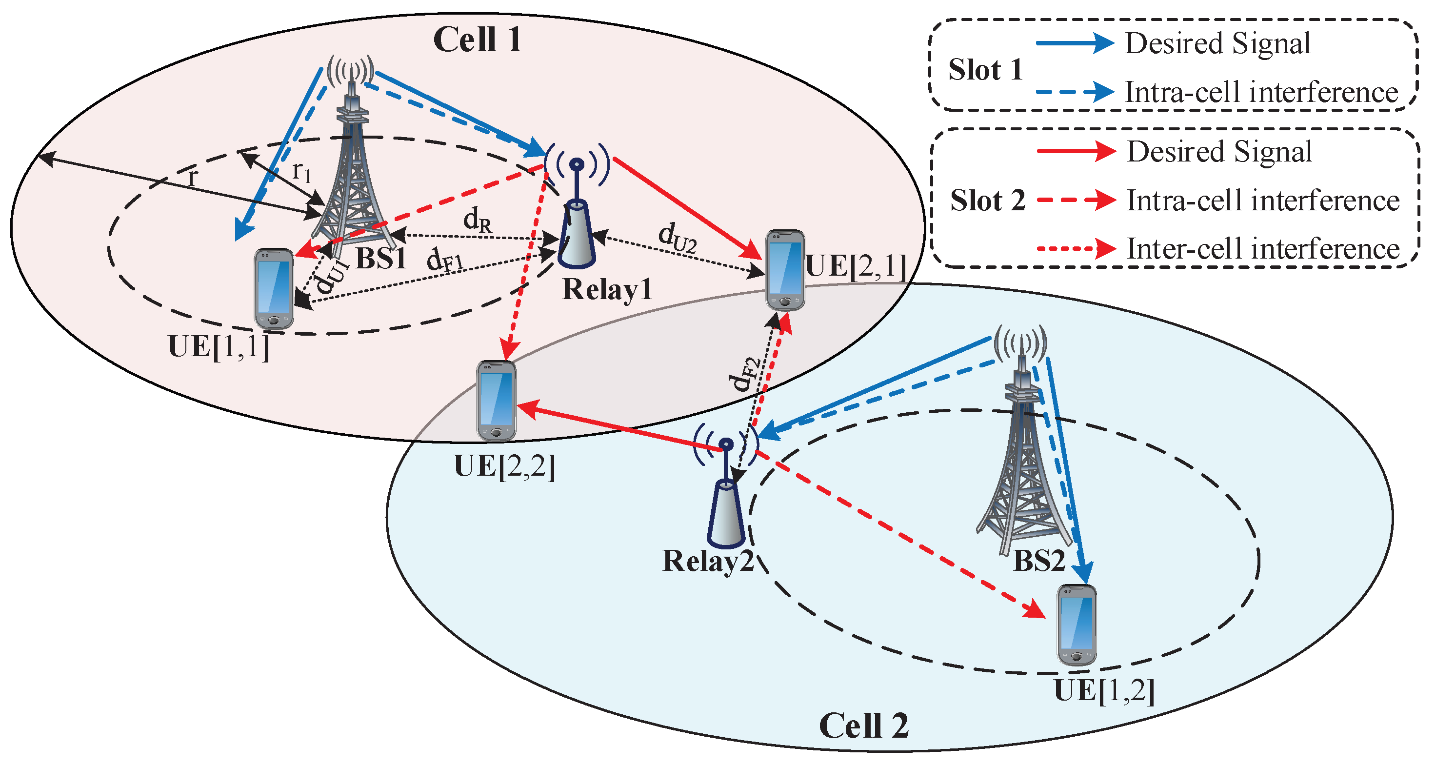
The specific two-cell relay HetNet with two communication phases is illustrated in Figure 1. Both the relay and CCU are connected directly to the BS. The relay is located at $d_R$ away from BS, while the CCU is randomly distributed in the center area within the radius of $d_{U1},(d_{U1}\le r_1)$, the distance between them being $d_{F1}$. The CEU communicates with the base station through the relay, $d_{U2}$ away from it. Meanwhile, the CEU is interfered by the relay in the adjacent cell at a distance of $d_{F2}$. We assume that the number of antennas configured at the transmitting (both BSs and relays) and receiving nodes (CCUs and CEUs) are M and N, respectively. Without loss of generality, all the nodes work on the same spectrum for each phase of downlink transmission. The AF-mode relay only forwards the received signals through a processing matrix without decoding them.

As shown in Figure 1, the whole transmission period is partitioned into two sub-time slots and the i-th $(i=1,2)$ user in the l-th cell is denoted as UE[$i,l$]. In particular, we assume that the Rayleigh channel model is static during a whole transmission period and the global CSI is obtained by the BSs and CEUs in the network. Because the transmit beamforming matrix at each BS is obtained through the closed-form method as in Reference [5,6], it requires the inter-cell and intra-cell interference channels to be known to the BS. Furthermore, note that we define the local CSI as the channel information shared only in the same cell, which is not available in adjacent cells. For relays and CCUs, only local CSI needs to be known, since the inter-cell interference has no influence on them, and they are able to align intra-cell interference to the desired signal subspace without inter-cell CSI.

Taking the communications in Cell 1 as an example, in sub-time slot 1, when BS1 transmits $N_s$ data streams to its users (i.e., UE[$1,1$], UE[$2,1$]), the intra-cell interference will be generated between UE[$1,1$] and Relay 1. The received signals at these two nodes can be expressed as

$${\mathbf{y}}_{t1}^{[1,1]}=\sqrt{g_1^{[1,1]}}{\mathbf{H}}_1^{[1,1]}({\mathbf{V}}^{[1,1]}{\mathbf{s}}_{t1}^{[1,1]}+{\mathbf{V}}^{[2,1]}{\mathbf{s}}_{t1}^{[2,1]})+{\mathbf{n}}_{t1}^{[1,1]},$$

(1)

$${\mathbf{y}}_{t1}^{R1}=\sqrt{g_1^{R1}}{\mathbf{H}}_1^{R1}({\mathbf{V}}^{[2,1]}{\mathbf{s}}_{t1}^{[2,1]}+{\mathbf{V}}^{[1,1]}{\mathbf{s}}_{t1}^{[1,1]})+{\mathbf{n}}_{t1}^{R1},$$

(2)

where ${\mathbf{H}}_j^{[i,l]}\in {\mathbb{C}}^{N\times N},i,j,l\in \{1,2\}$ and ${\mathbf{H}}_j^{Ri}\in {\mathbb{C}}^{N\times N},i,j\in \{1,2\}$ stand for the channel matrices from BS j to UE[$i,l$] and relay i, respectively. $\sqrt{g_j^{[i,l]}}$ and $\sqrt{g_j^{Ri}}$ denote the long term path gain from BS j to UE[$i,l$] and to relay i. ${\mathbf{V}}^{[i,l]}\in {\mathbb{C}}^{M\times N_s},{\mathbf{V}}^{[i,l]H}{\mathbf{V}}^{[i,l]}={\mathbf{I}}_{N_s}$ is the transmit beamforming matrix towards UE[$i,l$]. The desired signal vector and additive white Gaussian noise (AWGN) vector with variance ${\sigma }^2$ in sub-time slot $tj$ at UE[$i,l$] are denoted as $N_s\times 1$ vectors ${\mathbf{s}}_{tj}^{[i,l]}$ and ${\mathbf{n}}_{tj}^{[i,l]}$.

In sub-time slot 2, Relay 1 forwards the combined signal to UE[2,1]. However, it should be noticed that UE[2,1] will also receive the inter-cell interference from Relay 2 in Cell 2, which is given by

$$\begin{array}{cc}{\mathbf{y}}_{t2}^{[2,1]}\hfill & =\sqrt{g_{R1}^{[2,1]}}{\mathbf{H}}_{R1}^{[2,1]}{\mathbf{G}}_1{\rho }_{\left(R_1\right)}{\mathbf{y}}_{t1}^{R1}+\sqrt{g_{R2}^{[2,1]}}{\mathbf{H}}_{R2}^{[2,1]}{\mathbf{G}}_2{\rho }_{\left(R_2\right)}{\mathbf{y}}_{t1}^{R2}\hfill \\ & +{\mathbf{n}}_{t2}^{[2,1]},\hfill \end{array}$$

(3)

where ${\mathbf{G}}_i\in {\mathbb{C}}^{N\times N}$, $i\in \{1,2\}$ and ${\rho }_{\left(R_i\right)}^2=\frac{P_{t\left(R_i\right)}}{g_i^{R_i}tr({\mathbf{H}}_i^{R_i}{\mathbf{V}}^{[2,i]}{\mathbf{V}}^{[2,i]H}{\mathbf{H}}_i^{R_{i}H}+{\mathbf{H}}_i^{R_i}{\mathbf{V}}^{[1,i]}{\mathbf{V}}^{[1,i]H}{\mathbf{H}}_i^{R_{i}H})\frac{P_{t\left(i\right)}}{N_s}+N_s{\sigma }^2}$ are the processing matrices and the relay amplification factors, respectively. Specifically, $P_{t\left(Ri\right)}$ and $P_{t\left(i\right)}$ are the transmit power at relay i and BS i, respectively. According to Reference [18], the selection of ${\rho }_{\left(R_i\right)}^2$ aims at inverting the fading effect of the first channel and limiting the output power of the relay if the fading amplitude of the first hop is low. Since Relay 1 works in half-duplex mode, we assume that BS1 only transmits signal to UE[1,1] in sub-time slot 2. However, the combined signal received by UE[1,1] contains the intra-cell interference caused by Relay 1, which can be denoted as

$$\begin{array}{cc}{\mathbf{y}}_{t2}^{[1,1]}\hfill & =\sqrt{g_1^{[1,1]}}{\mathbf{H}}_1^{[1,1]}{\mathbf{V}}^{[1,1]}{\mathbf{s}}_{t2}^{[1,1]}+\sqrt{g_{R1}^{[1,1]}}{\rho }_{\left(R_1\right)}{\mathbf{H}}_{R1}^{[1,1]}{\mathbf{G}}_1{\mathbf{y}}_{t1}^{R1}\hfill \\ & +{\mathbf{n}}_{t2}^{[1,1]}.\hfill \end{array}$$

(4)

In order to mitigate the intra-cell and inter-cell interference, we use the receive beamforming matrix at each user to receive the combined signal. The received signal after decoding in sub-time slot $t1$ can be expressed as

$${\tilde{\mathbf{y}}}_{t1}^{[1,1]}={\mathbf{U}}^{[1,1]H}\sqrt{g_1^{[1,1]}}{\mathbf{H}}_1^{[1,1]}{\mathbf{V}}^{[1,1]}{\mathbf{s}}_{t1}^{[1,1]}+{\mathbf{U}}^{[1,1]H}\sqrt{g_1^{[1,1]}}{\mathbf{H}}_1^{[1,1]}{\mathbf{V}}^{[2,1]}{\mathbf{s}}_{t1}^{[2,1]}+{\mathbf{U}}^{[1,1]H}{\mathbf{n}}_{t1}^{[1,1]},$$

(5)

and in sub-time slot $t2$ as

$$\begin{array}{cc}{\tilde{\mathbf{y}}}_{t2}^{[2,1]}\hfill & =\sqrt{g_{R1}^{[2,1]}}{\mathbf{U}}^{[2,1]H}{\mathbf{H}}_{R1}^{[2,1]}{\mathbf{G}}_1{\rho }_{\left(R1\right)}{\mathbf{y}}_{t1}^{R1}+\sqrt{g_{R2}^{[2,1]}}{\mathbf{U}}^{[2,1]H}{\mathbf{H}}_{R2}^{[2,1]}{\mathbf{G}}_2{\rho }_{\left(R2\right)}{\mathbf{y}}_{t1}^{R2}+{\mathbf{U}}^{[2,1]H}{\mathbf{n}}_{t2}^{[2,1]}\hfill \\ & =\sqrt{g_{R1}^{[2,1]}{g}_1^{R1}}{\rho }_{\left(R1\right)}{\mathbf{U}}^{[2,1]H}{\mathbf{H}}_{R1}^{[2,1]}{\mathbf{G}}_1{\mathbf{H}}_1^{R1}{\mathbf{V}}^{[2,1]}{\mathbf{s}}_{t1}^{[2,1]}+\sqrt{g_{R1}^{[2,1]}{g}_1^{R1}}{\rho }_{\left(R1\right)}{\mathbf{U}}^{[2,1]H}{\mathbf{H}}_{R1}^{[2,1]}{\mathbf{G}}_1{\mathbf{H}}_1^{R1}{\mathbf{V}}^{[1,1]}{\mathbf{s}}_{t1}^{[1,1]}\\ & +\sqrt{g_{R2}^{[2,1]}{g}_2^{R2}}{\rho }_{\left(R2\right)}{\mathbf{U}}^{[2,1]H}{\mathbf{H}}_{R2}^{[2,1]}{\mathbf{G}}_2{\mathbf{H}}_2^{R2}{\mathbf{V}}^{[2,2]}{\mathbf{s}}_{t1}^{[2,2]}+\sqrt{g_{R2}^{[2,1]}{g}_2^{R2}}{\rho }_{\left(R2\right)}{\mathbf{U}}^{[2,1]H}{\mathbf{H}}_{R2}^{[2,1]}{\mathbf{G}}_2{\mathbf{H}}_2^{R2}{\mathbf{V}}^{[1,2]}{\mathbf{s}}_{t1}^{[1,2]}\hfill \\ & +\sqrt{g_{R1}^{[2,1]}}{\mathbf{U}}^{[2,1]H}{\mathbf{H}}_{R1}^{[2,1]}{\mathbf{G}}_1{\rho }_{\left(R1\right)}{\mathbf{n}}_{t1}^{R1}+\sqrt{g_{R2}^{[2,1]}}{\mathbf{U}}^{[2,1]H}{\mathbf{H}}_{R2}^{[2,1]}{\mathbf{G}}_2{\rho }_{\left(R2\right)}{\mathbf{n}}_{t1}^{R2}+{\mathbf{U}}^{[2,1]H}{\mathbf{n}}_{t2}^{[2,1]},\hfill \end{array}$$

(6)

$$\begin{array}{cc}{\tilde{\mathbf{y}}}_{t2}^{[1,1]}\hfill & =\sqrt{g_1^{[1,1]}}{\mathbf{U}}^{[1,1]H}{\mathbf{H}}_1^{[1,1]}{\mathbf{V}}^{[1,1]}{\mathbf{s}}_{t2}^{[1,1]}+\sqrt{g_{R1}^{[1,1]}}{\mathbf{U}}^{[1,1]H}{\mathbf{H}}_{R1}^{[1,1]}{\mathbf{G}}_1{\mathbf{y}}_{t1}^{R1}+{\mathbf{U}}^{[1,1]H}{\mathbf{n}}_{t2}^{[1,1]}\hfill \\ & =\sqrt{g_1^{[1,1]}}{\mathbf{U}}^{[1,1]H}{\mathbf{H}}_1^{[1,1]}{\mathbf{V}}^{[1,1]}{\mathbf{s}}_{t2}^{[1,1]}+\sqrt{g_{R1}^{[1,1]}{g}_1^{R1}}{\rho }_{\left(R1\right)}{\mathbf{U}}^{[1,1]H}{\mathbf{H}}_{R1}^{[1,1]}{\mathbf{G}}_1{\mathbf{H}}_1^{R1}{\mathbf{V}}^{[2,1]}{\mathbf{s}}_{t1}^{[2,1]}\hfill \\ & +\sqrt{g_{R1}^{[1,1]}{g}_1^{R1}}{\rho }_{\left(R1\right)}{\mathbf{U}}^{[1,1]H}{\mathbf{H}}_{R1}^{[1,1]}{\mathbf{G}}_1{\mathbf{H}}_1^{R1}{\mathbf{V}}^{[1,1]}{\mathbf{s}}_{t1}^{[1,1]}+\sqrt{g_{R1}^{[1,1]}}{\mathbf{U}}^{[1,1]H}{\mathbf{H}}_{R1}^{[1,1]}{\mathbf{G}}_1{\mathbf{n}}_{t1}^{R1}+{\mathbf{U}}^{[1,1]H}{\mathbf{n}}_{t2}^{[1,1]},\hfill \end{array}$$

(7)

where ${\mathbf{U}}^{[i,1]}\in {\mathbb{C}}^{N\times N_s},{\mathbf{U}}^{[i,l]H}{\mathbf{U}}^{[i,l]}={\mathbf{I}}_{N_s}$ is the receive beamforming matrix and ${\tilde{\mathbf{n}}}_{tj}^{[i,1]}={\mathbf{U}}^{[i,1]}{\mathbf{n}}_{tj}^{[i,1]}$ is the effective noise vector of the i-th user in Cell 1. Details on the design of the proposed TPIA scheme are introduced in the next section.

3. The Cross Time Slot Partial Interference Alignment

Since the intra-cell interference from relay to CCU in sub-time slot 2 contains the desired signal from BS to CCU in sub-time slot 1, we extract and align this part of the interference to the desired signal subspace at the CCU in sub-time slot 2 (i.e., the cross time slot alignment). Then, a partial IA scheme is proposed to deal with the intra-cell and inter-cell interference at the CEUs. Taking Cell 1 as an example, the details are given as below.

3.1. The Processing Matrix at Relay

We design the processing matrix at Relay 1 by aligning part of the intra-cell interference (i.e., the desired signal sent to UE[1,1] in sub-time slot 1) to the desired signal subspace during the signal transmission to UE[1,1] in sub-time slot 2. According to (7), we have

$$span({\mathbf{H}}_1^{[1,1]}{\mathbf{V}}^{[1,1]})=span({\mathbf{H}}_{R1}^{[1,1]}{\mathbf{G}}_1{\mathbf{H}}_1^{\left[R1\right]}{\mathbf{V}}^{[1,1]}).$$

(8)

Hence, the processing matrix on relay 1 can be obtained as

$$span({\mathbf{G}}_1)=span({\mathbf{H}}_{R1}^{[1,1]-1}{\mathbf{H}}_1^{[1,1]}{\mathbf{H}}_1^{\left[R1\right]-1}).$$

(9)

As mentioned above, the desired signals to UE[1,1] in two sub-time slots are aligned to the same subspace. UE[1,1] can directly mitigate the interference by decoding the combined signal. Similarly in Cell 2, the processing matrix of Relay 2 can be obtained, i.e.,

$$span({\mathbf{G}}_2)=span({\mathbf{H}}_{R2}^{[1,2]-1}{\mathbf{H}}_2^{[1,2]}{\mathbf{H}}_2^{\left[R2\right]-1}).$$

(10)

3.2. Partial Interference Alignment for the CEU

According to (6), the signal transmitted to UE[2,1] will be interfered with by the intra-cell interference contained in the combined signal and the inter-cell interference caused by Relay 2 in Cell 2. Note that the inter-cell interference contains signals to both the CCU and CEU (i.e., ${\mathbf{s}}_{t1}^{[1,2]}$ and ${\mathbf{s}}_{t1}^{[2,2]}$) in sub-time slot 1. These two signals are carried by different transmit beamforming matrices, which means they cannot be aligned to the same subspace. Hence, we choose to align one of them to the intra-cell interference subspace. For example, we align the intra-cell interference ${\mathbf{s}}_{t1}^{[1,1]}$ and inter-cell interference ${\mathbf{s}}_{t1}^{[2,2]}$ to the same subspace such that

$$span({\mathbf{H}}_{R1}^{[2,1]}{\mathbf{G}}_1{\mathbf{H}}_1^{R1}{\mathbf{V}}^{[1,1]})=span({\mathbf{H}}_{R2}^{[2,1]}{\mathbf{G}}_2{\mathbf{H}}_2^{R2}{\mathbf{V}}^{[2,2]}).$$

(11)

As in Cell 2, by aligning the intra-cell end inter-cell interference at UE[2,2], we can obtain the transmit beamforming matrix to UE[2,1], i.e.,

$$span({\mathbf{H}}_{R1}^{[2,2]}{\mathbf{G}}_1{\mathbf{H}}_1^{R1}{\mathbf{V}}^{[2,1]})=span({\mathbf{H}}_{R2}^{[2,2]}{\mathbf{G}}_2{\mathbf{H}}_2^{R2}{\mathbf{V}}^{[1,2]}).$$

(12)

3.3. Nullifying Inter-Cell and Intra-Cell Interference

To ensure the desired signal can be received without interference, we need to design the receive beamforming matrix at each user. According to (7), although the desired signals to the same CCU in different sub-time slots are aligned by relay, the aligned signal to UE[1,1] still overlaps with the interference caused by Relay 1. Furthermore, the interference in sub-time slot 1 should also be considered when designing the receive beamforming matrix.

3.3.1. Receive Beamforming Matrix at Each User

The desired signal and the intra-cell interference in the two sub-time slots are aligned to the same subspace as well. Hence, the receive beamforming matrix for UE[1,1] can be obtained as

$${\mathbf{U}}^{[1,1]}=null\left({[{\mathbf{H}}_1^{[1,1]}{\mathbf{V}}^{[2,1]}]}^H\right).$$

(13)

On the basis of (11), part of the inter-cell and the intra-cell interference have been aligned in the same subspace. Now, we need to design the receive beamforming matrix at UE[2,1] to mitigate both the remaining inter-cell and the aligned interference, i.e.,

$${\mathbf{U}}^{[2,1]}=null\left({[{\mathbf{H}}_{R1}^{[2,1]}{\mathbf{G}}_1{\mathbf{H}}_1^{R1}{\mathbf{V}}^{[1,1]},{\mathbf{H}}_{R2}^{[2,1]}{\mathbf{G}}_2{\mathbf{H}}_2^{R2}{\mathbf{V}}^{[1,2]}]}^H\right).$$

(14)

As in Cell 2, the receive beamforming matrix for the two users can be achieved as

$${\mathbf{U}}^{[1,2]}=null\left({[{\mathbf{H}}_1^{[1,2]}{\mathbf{V}}^{[2,2]}]}^H\right),$$

(15)

$${\mathbf{U}}^{[2,2]}=null\left({[{\mathbf{H}}_{R2}^{[2,2]}{\mathbf{G}}_2{\mathbf{H}}_2^{R2}{\mathbf{V}}^{[1,2]},{\mathbf{H}}_{R1}^{[2,2]}{\mathbf{G}}_1{\mathbf{H}}_1^{R1}{\mathbf{V}}^{[1,1]}]}^H\right).$$

(16)

3.3.2. Feasibility Condition

Proposition 1.

To guarantee the existence of nonzero solutions for each receive beamforming matrix, the number of antennas configured on each node should satisfy

$$N\ge 3N_s,M\ge 2N_s.$$

(17)

Proof. 

Firstly, we define the matrices in (13) and (14) as

$${\mathbf{F}}^{[1,1]}={[{\mathbf{H}}_1^{[1,1]}{\mathbf{V}}^{[2,1]}]}^H,$$

(18)

$${\mathbf{F}}^{[2,1]}={[{\mathbf{H}}_{R1}^{[2,1]}{\mathbf{G}}_1{\mathbf{H}}_1^{R1}{\mathbf{V}}^{[1,1]},{\mathbf{H}}_{R2}^{[2,1]}{\mathbf{G}}_2{\mathbf{H}}_2^{R2}{\mathbf{V}}^{[1,2]}]}^H.$$

(19)

Since the Rayleigh channel model is adopted and the channel elements are independently distributed, ${\mathbf{F}}^{[1,1]}$ and ${\mathbf{F}}^{[2,1]}$ are the full rank matrices, i.e., $rank({\mathbf{F}}^{[1,1]})=min(N_s,N)$ and $rank({\mathbf{F}}^{[2,1]})=min(2N_s,N)$. The number of transmit antennas can be derived from (11) or (12), which can be solved through the close-formed method as in Reference [6]. To guarantee the existence of $N_s$ nonzero solutions, we have

$$N-max(rank({\mathbf{F}}^{[1,1]}),rank({\mathbf{F}}^{[2,1]}))\ge N_s,i.e.,N\ge 3N_s,$$

(20)

$$2M-N\ge N_s,i.e.,M\ge 2N_s.$$

(21)

The proposition has been proved. □

3.4. The Number of Achievable SDoF

According to References [5,6], the SDoF is defined as the pre-log factor of the sum rate during a unit time period. However, since the transmission period in our paper is divided into two parts (each part containing one sub-time slot), we define the achievable SDoF as the ratio of the total number of DoF to the number of sub-time slots, i.e.,

$$SDoF=\underset{SNR\to \infty }{lim}\frac{R_{\sum }\left(t\right)}{log\left(SNR\right)\sum t}=\frac{\sum N_s^{[i,l]}\left(t\right)}{\sum t},$$

(22)

where $R_{\sum }\left(t\right)={\sum }_{i=1}^2{\sum }_{l=1}^2{R}^{[i,l]}\left(t\right)={\sum }_{i=1}^2{\sum }_{l=1}^{2}lo{g}_2\left(1+SIN{R}_{[i,l]}\left(t\right)\right)$ and $N_s^{[i,l]}\left(t\right)$ represent the sum-rate performance and the number of data streams to UE[$i,l$] in sub-time slot t, respectively. As can be found from (20) and (21), the antenna configurations at each receiver (i.e., CEU) is bigger than that at the transmitters (i.e., BS and relay) due to the influence from both inter-cell and intra-cell interference. Here, we take the number of transmit antennas M as an example. In the first sub-time slot, two CCUs are served simultaneously, the number of data streams decoded at each one is $M/2$, yielding $M/2\times 2=M$ DoF. Note that we assume the number of antennas configured at each CEU is big enough to decode the received data streams. Hence, in the second sub-time slot, each CEU can also achieve $M/2$ DoF. Since the two CCUs are also served by the BSs in the second sub-time slot, the achievable SDoF in the whole transmission period can be derived as

$$SDoF=\frac{M+2\ast M/2+M}{2}=\frac{3M}{2}.$$

(23)

4. Simulation Results

In this section, we firstly compare the achievable DoF and sum-rate performance between TPIA and other conventional schemes. Then, the average rate performance of the CCU and CEU are simulated and analyzed to support the explanation of the system model. The simulation parameters are listed in

Table 1. Simulation Configurations.

Parameter	Assumption
Radius of cell $\left(r\right)$	500 m
Radius of center area $\left(r_1\right)$	250 m
Distances among nodes ($d_1$, $d_2$, $d_R$, $d_{F_1}$, $d_{F_2}$)	200 m, 30 m, 400 m, 300 m, 50 m
Carrier frequency / Bandwidth	2 GHz/10 MHz
Maximum transmit power of base atation (BS)	46 dBm
Maximum transmit power of relay	18 dBm
The number of antennas at BS	2
The number of antennas at Relay	2
The number of antennas at user equipment (UE)	3
degrees of freedom (DoF) of each transmission link	1
Path loss from BS to user	128.1 + 37.6log10R [dB], R in km
Path loss from relay to user	140.7 + 36.7log10R [dB], R in km
Antenna pattern	0 dB (omni-directional)

. Specifically, the signal to noise ratio (SNR) in the simulation is defined as the ratio of transmit power to the power of noise. The transmit power at each BS and relay is set to the maximum value (i.e., the simulation parameters in Table 1), and the power of noise at CCU and CEU vary according to $P_{N\left(CCU\right)}=P_{BS}-SNR\left(dB\right)$ and $P_{N\left(CEU\right)}=P_{relay}-SNR\left(dB\right)$, respectively. Furthermore, the lower complexity and ease of deployment make the relays with fixed amplification factors attractive from a practical standpoint. Hence, the influence of fixed amplification factor is analyzed and three fixed values of relay amplification factors are selected for simulation simplicity in this section. It should be noted that the power of noise at the CEU varies according to $P_{N\left(CEU\right)}=P_{relay}\left(\rho \right)-SNR\left(dB\right)$, since the transmit power of the relay is decided by the fixed amplification factor. The channels among different nodes are assumed to be uncorrelated and the average simulation results are computed under 1000 channel instances.

The achievable SDoF and sum-rate comparison of different schemes are shown in

Table 2. Achievable SDoF comparison of different schemes.

Scheme	Number of Sub-Time Slots	SDoF
time division multiple address (TDMA)	3	4/3
Alternate [2]	3	5/3
Extended methods e.g., zero-forcing (ZF), methods in [5,6,10]	3	2
TPIA (proposed)	2	3

and Figure 2, respectively. We assumed the amplification factor to be variable to maintain the maximum transmit power of relay. It can obviously be seen that the TPIA scheme utilizes less sub-time slots than others and obtains the highest SDoF and sum-rate performance. That is because both intra-cell and inter-cell interference are simultaneously mitigated in only two sub-time slots per transmission period while other schemes need an extra sub-time slot to avoid the intra-cell interference caused by the BS. Furthermore, our method can effectively decrease the cost caused by synchronization because of the smaller number of time partition.

In Figure 3, we plot the average rate comparison between CCU and CEU to analyze the proposed TPIA scheme based on the system model. As can be seen from the figure, the average rate curve of the CCU is obviously higher than that of the CEU, especially at the high SNR region. That is because the data transmission from BS to CCU is performed in both two sub-time slots (i.e., Formulas (5) and (7) in Section 2), while the relay only transmits a signal to the CEU in the second sub-time slot (i.e., Formula (6) in Section 2). Additionally, the average rate increase is faster than that of the CEU, since part of the intra-cell interference is aligned to the desired signal subspace and both the two aligned signals to CCU increase with SNR, which results in a significant improvement of receive power at each CCU. Furthermore, the combined signal forwarded by the relay to the CEU in each cell contains inter-cell interference and more kinds of noise (details are given in Formula (6) in Section 2), all of which increase with the SNR. Hence, the average rate of the CEU gradually approaches the ceiling with increasing SNR.

The Average rate of TPIA versus SNR under different amplification factors is shown in Figure 4. It is based on the assumption that the location of each user is invariable (i.e., in Table 1) and the channel is static during each transmission period. As can be seen from the figure, the achievable rate decreases with the increase in amplification factor. That is because the average rate increment at CEU is lower than the decrement at CCU, although both of the desired signal and interference (inter-cell and intra-cell interference) are enhanced by the relay.

5. Conclusions

In this paper, we propose using the TPIA to mitigate both the inter-cell and intra-cell interference simultaneously in a two-cell relay HetNet. Furthermore, a higher SDoF and sum rate were obtained, and the influence of the fixed amplification factor on the average rate performance were analyzed. This method can be deployed in space-limited transceiver design. Extending the proposed method to a multi-cell scenario, which is more practical, will be considered in our future works.

References

1. Shin, W.; Lee, N.; Yang, H.; Lee, J. Relay-Aided Successive Aligned Interference Cancellation for Wireless X Networks with Full-Duplex Relays. IEEE Trans. Veh. Technol. 2017, 66, 421–432. [Google Scholar] [CrossRef]
2. Zhou, M.; Li, H.; Li, J.; Suo, L.; Shao, W. On Feasibility of Interference Alignment in Full-Duplex-Based Small Cell Networks. IEEE Commun. Lett. 2017, 21, 2294–2297. [Google Scholar] [CrossRef]
3. Gomadam, K.; Cadambe, V.R.; Jafar, S.A. A distributed numerical approach to interference alignment and applications to wireless interference networks. IEEE Commun. Lett. 2011, 57, 3309–3322. [Google Scholar] [CrossRef]
4. Tang, J.; Lambotharan, S. Interference Alignment Techniques for MIMO Multi-Cell Interfering Broadcast Channels. IEEE Trans. Commun. 2013, 61, 164–175. [Google Scholar] [CrossRef]
5. Cao, P.; Zappone, A.; Jorswieck, A.E. Grouping-Based Interference Alignment with IA-Cell Assignment 136 in Multi-Cell MIMO MAC Under Limited Feedback. IEEE Trans. Signal Process. 2016, 64, 1336–1351. [Google Scholar] [CrossRef]
6. Wang, C.; Qin, C.; Yao, Y.; Li, Y.; Wang, W. Low Complexity Interference Alignment for mmWave MIMO Channels in Three-Cell Mobile Network. IEEE J. Sel. Areas Commun. 2017, 35, 1513–1523. [Google Scholar] [CrossRef]
7. Castanheira, D.; Silva, A.; Gameiro, A. Retrospective Interference Alignment: Degrees of Freedom Scaling with Distributed Transmitters. IEEE Trans. Inf. Theory 2017, 63, 1721–1730. [Google Scholar] [CrossRef]
8. Maso, M.; Debbah, M.; Vangelista, L. A Distributed Approach to Interference Alignment in OFDM-Based Two-Tiered Networks. IEEE Trans. Veh. Technol. 2013, 62, 1935–1949. [Google Scholar] [CrossRef] [Green Version]
9. Castanheira, D.; Silva, A.; Dinis, R.; Gameiro, A. Efficient Transmitter and Receiver Designs for SC-FDMA Based Heterogeneous Networks. IEEE Trans. Commun. 2015, 63, 2500–2510. [Google Scholar] [CrossRef]
10. Jin, J.; Gao, X.C.; Li, X.; Li, S.; Wang, Z. Achievable Degrees of Freedom for the Two-Cell Two-Hop MIMO Interference Channel with Half-Duplex Relays. IEEE Access. 2017, 5, 1376–1381. [Google Scholar] [CrossRef]
11. Cadambe, V.R.; Jafar, S.A. Interference Alignment and the Degrees of Freedom of Wireless X Networks. IEEE Trans. Inf. Theory 2009, 55, 3893–3908. [Google Scholar] [CrossRef]
12. Gou, T.; Jafar, S.; Wei, C.; Jeon, S.; Chung, S. Aligned interference neutralization and the degrees of freedom of the 2 × 2 × 2 interference channel. IEEE Trans. Inf. Theory 2012, 58, 4381–4395. [Google Scholar] [CrossRef]
13. Jeon, S.; Chung, S.; Jafar, S. Degrees of freedom of multi-source relay networks. In Proceedings of the 2009 47th Annual Allerton Conference on Communication, Control, and Computing, Monticello, IL, USA, 30 September–2 October 2009; pp. 388–393. [Google Scholar]
14. Lee, N.; Heath, R. Degrees of freedom for the two-cell two-hop MIMO interference channel: Interference-free relay transmission and spectrally efficient relaying protocol. IEEE Trans. Inf. Theory 2013, 59, 2882–2896. [Google Scholar] [CrossRef]
15. Shomorony, I.; Avestimehr, A. Degrees of freedom of two-hop wireless network: Everyone gets the entire cake. IEEE Trans. Inf. Theory 2014, 60, 2417–2431. [Google Scholar] [CrossRef]
16. Rankov, B.; Wittneben, A. Spectral efficient protocols for halfduplex fading relay channels. IEEE J. Sel. Areas Commun. 2007, 25, 379–389. [Google Scholar] [CrossRef]
17. Li, X.; Sun, Y.; Zhao, N.; Yu, F.R.; Xu, Z. A Novel Interference Alignment Scheme with a Full-Duplex MIMO Relay. IEEE Commun. Lett. 2015, 19, 1798–1801. [Google Scholar] [CrossRef]
18. Hasna, M.O.; Alouini, M.S. A performance study of dual-hop transmissions with fixed gain relays. IEEE Trans. Wirel. Commun. 2004, 3, 1963–1968. [Google Scholar] [CrossRef]
Figure 1. System model of two-cell relay heterogeneous network (HetNet).
Applsci 09 00652 g001
Figure 2. Achievable sum-rate versus signal to noise ratio (SNR) comparison of different schemes.
Applsci 09 00652 g002
Figure 3. Average rate comparison under TPIA between cell-center user (CCU) and cell-edge user (CEU).
Applsci 09 00652 g003
Figure 4. The average rate of TPIA in sub-time slot 2 under different amplification factors.
Applsci 09 00652 g004