A Frequency–Power Droop Coefficient Determination Method of Mixed Line-Commutated and Voltage-Sourced Converter Multi-Infeed, High-Voltage, Direct Current Systems: An Actual Case Study in Korea

Abstract

Among the grid service applications of high-voltage direct current (HVDC) systems, frequency–power droop control for islanded networks is one of the most widely used schemes. In this paper, a new frequency-power droop coefficient determination method for a mixed line-commutated converter (LCC) and voltage-sourced converter (VSC)-based multi-infeed HVDC (MIDC) system is proposed. The proposed method is designed for the minimization of power loss. An interior-point method is used as an optimization algorithm to implement the proposed scheduling method, and the droop coefficients of the HVDCs are determined graphically using the Monte Carlo sampling method. Two test systems—the modified Institute of Electrical and Electronics Engineers (IEEE) 14-bus system and an actual Jeju Island network in Korea—were utilized for MATLAB simulation case studies, to demonstrate that the proposed method is effective for reducing power system loss during frequency control.

1. Introduction

High-voltage direct current (HVDC) systems have played an important role in sub-marine power transmission, due to economic advantages over their alternating current (AC) counterparts [1]. Nowadays, due to the complexity of modern power systems, HVDC systems are adopted in practice, not only for constant power delivery between massive networks, but also to provide grid services for island grids [2,3,4,5,6,7,8]. For example, in Korea, two line-commutated converter (LCC) HVDCs, the 180-kV/300-MW Haenam–Jeju HVDC [9] and ±250 kV/400 MW Jindo–Jeju HVDC [10], were constructed by the Korea Electric Power Corporation (KEPCO) for supporting Jeju Island and integrating massive wind power plants. Furthermore, KEPCO is planning to construct one more ±150 kV/200 MW voltage-sourced converter (VSC) HVDC between the main grid and Jeju Island [11].

With the technical development of both the LCC and VSC HVDC systems, there are numerous island networks with multi-infeed HVDC (MIDC) systems, encompassing both types of HVDCs, similar to the Jeju Island case. According to trends, many studies have concentrated on the MIDC systems [12,13,14,15,16]. Major research effort has been focused on the stable operation of the MIDC systems by introducing novel indexes, such as the multi-infeed interaction factor (MIIF), multi-infeed effective short-circuit ratio (MIESCR) [12], apparent increase in short-circuit ratio (AISCR) [13], and improved effective short-circuit ratio (IESCR) [14]. In parallel with such research, some studies have concentrated on the economic operation of MIDC systems, which is represented by optimal power flow (OPF) [17,18,19,20]. In two such studies [17,18], steady-state VSC–HVDC modeling methods and OPF formulations based on the Newton–Raphson method are proposed. Although only a single HVDC system is considered in these studies [17,18], the principle can be easily expanded to MIDC systems. In one study [19], a loss minimization method with an AC/DC hybrid grid incorporating only VSC HVDCs is proposed, based on an interior-point method. In another study [20], a similar method adopting both LCC and VSC HVDC is proposed. However, the authors of the above studies only consider the steady-state values of the HVDC systems. Thus, if the load profiles were different from the forecasted value, the previous methods were unable to find the optimal set-point, because the forecasting error was not considered.

A common method used to satisfy the power balance between generation and load caused by the forecasting error is frequency–power droop control [21]. Similar to conventional generators, HVDC systems also adopt frequency–power droop controllers [22,23,24]. For economic operation of power systems during frequency control, the calculation of droop coefficients is a significant issue, and the coefficients are used to exploit multiple HVDC systems efficiently. It is practically important in the case of an islanded network, because the islanded system has a small load level and high renewable energy penetration, which cause high uncertainties in the power system. Due to those characteristics, off-nominal frequency situations occur more frequently, and the frequency deviation is more severe than the conventional large power network. In one study [25], an optimum calculation method of voltage–power droop coefficients for multi-terminal HVDC (MTDC) systems is proposed. However, the method could only be applied to the specific topology of the DC grid investigated in the paper. Another study proposes an optimization-based droop coefficient calculation method to maximize converter efficiencies for a low-voltage system [26]. A method to minimize DC transmission line loss using voltage–current droop coefficients has also been proposed [27]. The above research suggests that the droop coefficients of converters can be calculated by optimization of the problem. However, to our knowledge, optimization problems have rarely been suggested to calculate frequency–power droop coefficients of MIDC systems.

This paper suggests a method to determine the frequency–power droop coefficients of multiple HVDCs in MIDC systems. First, we propose an optimization problem for MIDC systems, to determine the operating points of HVDCs to minimize system loss. Using the results of the optimization problem, we propose a droop coefficient design method based on Monte Carlo sampling. The proposed method is verified by MATLAB simulation utilizing IEEE test systems and the actual networks of Jeju Island in Korea. Using our method, a system operator can define the operating points and droop coefficients of an MIDC system more efficiently.

2. Description of the Proposed Method

2.1. Optimazation Problem to Determine Operating Points

In this section, we formulate an optimization problem to determine the operating points of multiple HVDCs, including LCC and VSC HVDCs. This study is different from previous studies covering various type of HVDCs [22,23,24,25,27], because HVDCs can be regarded as active and reactive power sources in MIDC systems. Also, only the outputs of multiple HVDCs are considered in the optimization problem. In other words, generator outputs are considered as a constant in the problem.

2.1.1. Model Description

To formulate the constraints used in the optimization problem, power balance equations and converter models are required. In the case of the VSC, which can synthesize sine-wave AC voltage regardless of the residual network, the active and reactive power output—P_VSC and Q_VSC, respectively—are regulated independently [28]. Therefore, a VSC can be considered similar to a PQ load for the optimization, and the only consideration is the rated output power, as follows:

$$\sqrt{P_{VSC}^2(n)+Q_{VSC}^2(n)}<S_{VSC.rate}(n),$$

(1)

where S_VSC.rate(n) is the rated apparent power of the VSC HVDC connected to the n-th bus. Note that conversion loss of a VSC HVDC is ignored, because the input variables of controller are active and reactive power output at the inverter side. However, for future work, the conversion loss of VSC should be considered for solving overall optimization problems, including a DC system. The reactive power output of the LCC, Q_LCC, is different from the VSC, and cannot be regulated independent of the active power, P_LCC [29]. As conversion loss of LCC is less than 1% in general, the loss can be ignored [30]. Thus, Q_LCC can be presented as:

$$Q_{LCC}(n)=P_{LCC}(n)\tan \mathsf{\Phi }(n)$$

(2)

where Φ(n) is the power factor angle of LCC HVDC connected to the n-th bus. The power factor angle can be expressed as follows [31]:

$$\tan \mathsf{\Phi }(n)=\frac{2\mu (n)+\sin (2\alpha (n))-\sin (2\alpha (n)+2\mu (n))}{\cos (2\alpha (n))-\cos (2\alpha (n)+2\mu (n))}$$

(3)

where

$$\alpha (n)={\cos }^{-1}\left[\frac{\pi }{3\sqrt{2}B(n)T(n)V(n)}\left(V_{DC.rate}(n)+\frac{3X_C(n)P_{LCC}(n)}{\pi V_{DC.rate}(n)}\right)\right]$$

(4)

$$\mu (n)={\cos }^{-1}\left[\cos (\alpha (n))-\frac{\sqrt{2}{X}_C(n)P_{LCC}(n)}{B(n)T(n)V(n)V_{DC.rate}}\right]-\alpha$$

(5)

where V(n) represents voltage magnitude at n-th bus, and V_DC.rate(n) is the rated DC voltage of the LCC HVDC connected to the n-th bus. The transformer turn ratio and the number of six-pulse bridges at the n-th bus are represented by T(n) and B(n), respectively. The reactance of the converter transformer at the n-th bus is described by X_C(n). An inequality constraint of an LCC HVDC can be represented as

$$P_{LCC}(n)<P_{LCC.rate}(n)$$

(6)

where P_LCC.rate(n) is the rated active power of the LCC HVDC connected to n-th bus. Note that the index of the bus number (n) is utilized to express HVDC system connected to the n-th bus, which means multiple HVDCs can be considered in the proposed models, because each converter is connected to a different bus.

For every bus, the injected active (P) and reactive (Q) power, including generator output (P_GEN and Q_GEN), VSC output (P_VSC and Q_VSC), LCC output (P_LCC and Q_LCC), and connected load (P_LOAD and Q_LOAD) satisfy the following constraints [32]:

$$P_{GEN}(n)+P_{VSC}(n)+P_{LCC}(n)-P_{LOAD}(n)-{\displaystyle \sum _{k=1}^{N}V(n)V(k)\left\{G(n,k)\cos (\theta (n)-\theta (k))+B(n,k)\sin (\theta (n)-\theta (k))\right\}}=0$$

(7)

$$Q_{GEN}(n)+Q_{VSC}(n)+Q_{LCC}(n)-Q_{LOAD}(n)-{\displaystyle \sum _{k=1}^{N}V(n)V(k)\left\{G(n,k)\sin (\theta (n)-\theta (k))-B(n,k)\cos (\theta (n)-\theta (k))\right\}}=0$$

(8)

where the phase angle of n-th bus is represented by θ(n). An injected active and reactive power of the n-th bus can be represented by P(n) and Q(n), respectively. The real and imaginary parts of the admittance matrix between the n-th bus and k-th bus are represented as G(n,k) and B(n,k), respectively. If the generator, VSC, LCC, or load is not connected to bus n, the value of each symbol is zero. Note that P_GEN and Q_GEN are pre-determined by the system operator, and P_LOAD and Q_LOAD are previously forecasted values, which are considered as constant in the optimization problem. The security constraint of the AC voltage magnitude for per unit (p.u.) system can be represented as:

$$0.95\mathrm{p}.\mathrm{u}.<V(n)<1.05\mathrm{p}.\mathrm{u}.$$

(9)

2.1.2. Optimization Formulation and Solving Method

The vectors of the phase angle and voltage magnitude are represented as θ and V, respectively. The output references of VSC and LCC HVDCs can be represented by vector form, as P_VSC, Q_VSC, and P_LCC. Note that the reactive power of LCC HVDC, Q_LCC, can be represented in terms of P_LCC and V using Equations (2)–(5), so it is not necessary to include Q_LCC with the unknown vector. Therefore, the unknown vector, X, can be defined as:

$$X={\left[\begin{array}{ccccc}{P}_{VSC}^T& Q_{VSC}^T& P_{LCC}^T& {\mathsf{\theta }}^T& V^T\end{array}\right]}^T.$$

(10)

The purpose of the proposed problem is to minimize the system loss. Since conversion loss is not included in MIDC systems, only the line loss of AC systems is considered in the objective function. The objective function of the optimization is represented as:

$$\mathrm{minimize}f={\displaystyle \sum _{j=n}^N\left\{P_{GEN}(n)+P_{VSC}(n)+P_{LCC}(n)-P_{LOAD}(n)\right\}}$$

(11)

where N is the number of buses. Note that the difference between the active power injected to the network, P_GEN, P_VSC, P_LCC, and P_LOAD is the same as the system loss. Only LCC and VSC HVDCs are considered as frequency-supporting resources in this paper, with the assumption that conventional generators do not participate in frequency support. However, conventional generators can be considered in the optimization problem with a little modification, because the generators can be represented as active and reactive power sources similar to the VSC HVDC system. Additionally, the security constraint of the conventional generators can be represented by simple inequality of active and reactive power [33].

To solve the optimization problem, an interior-point method is used [34,35]. For the proposed optimization problem, an interior-point method cannot guarantee global optimality. However, as the solution found by the method is better than a trivial solution, the interior-point method can be successfully applied to the proposed optimization problem.

2.2. Frequency–Power Droop Coefficient Determination Method

In the optimization problem described in the previous section, the forecasted load profile is used to calculate the optimal operating points. However, load characteristics are different from the forecasted values, because there are uncertainties in the load forecasting procedure. Furthermore, uncertainty increases with the integration of bulk renewable energies [36]. In this situation, the outputs of multiple HVDCs form new operating points following droop characteristics, the coefficient of which is generally proportional to the capacities of the converters [37]. The conventional method for determining droop coefficients is simple, but the coefficients cannot create a more efficient solution. Therefore, a droop coefficient design method based on an optimization problem is required to operate MIDC systems more economically. We propose a statistical method to obtain optimal droop coefficients in this section.

2.2.1. Stochastic Optimization Based on the Monte Carlo Sampling Method

To determine the droop coefficient in the proposed method, the Monte Carlo sampling method was utilized [38]. In the Monte Carlo sampling method, a number of load profiles are generated and are utilized for solving the optimization problem. All cases are generated based on probabilistic function, such as normal distribution, to represent possible realizations in the presence of forecast errors. For each load profile, the optimization problem of the previous section is solved, and operating points of HVDCs are calculated. The sampling number is represented by i, and the output of LCC and VSC HVDCs connected to the n-th bus at the i-th sample is represented as P_VSC(n,i) and P_LCC(n,i), respectively.

Furthermore, frequency deviation for each load profile is also calculated in this stage. To derive frequency deviation, the relationship between load profile and grid frequency should be established. Therefore, on the assumption that only HVDCs participate in frequency regulation, we use the swing equations of the power network, including frequency-supporting HVDCs and a load with damping effects, as follows [21]:

$${\displaystyle \sum _{j=n}^N\left\{P_{GEN}(n,i)+P_{VSC}(n,i)+P_{LCC}(n,i)-P_{LOAD}(n,i)\right\}}=M_{eq}\frac{d\Delta \omega (i)}{dt}+D\Delta \omega (i)$$

(12)

where M_eq is the moment of inertia and D is the load damping coefficient. The deviation of grid frequency is represented by Δω. As the steady-state value (i.e., Δω = 0) of the left side of Equation (12) is equal to zero, and the active power of the HVDCs can be represented by the corresponding droop coefficients, the frequency deviation can be described as

$$\Delta \omega (i)=\frac{-{\displaystyle \sum _{n=1}^N\Delta P_{LOAD}(n,i)}}{{\displaystyle \sum _{n=1}^N\frac{1}{R_{VSC}(n)}}+{\displaystyle \sum _{n=1}^N\frac{1}{R_{LCC}(n)}}+D},$$

(13)

where ΔP_LOAD(n,i) is the change in the load profile of the n-th bus at the i-th sample, which is defined by the Monte Carlo sampling method. R_VSC(n) and R_LCC(n) represent the droop coefficient of the VSC and LCC HVDC connected to the n-th bus, respectively. The frequency deviation cannot be derived directly from Equation (13), because the droop coefficients of the HVDCs, which are not determined yet, are utilized to derive the frequency deviation. Therefore, we assume that the sum of coefficients is constant, as follows:

$${\displaystyle \sum _{n=1}^N\frac{1}{R_{VSC}(n)}}+{\displaystyle \sum _{n=1}^N\frac{1}{R_{LCC}(n)}}=\frac{1}{R_{eq}}$$

(14)

where R_eq is an equivalent droop coefficient of the total system. Note that the active power of HVDCs during grid frequency only depends on the ratio of the droop coefficient, so power sharing between multiple HVDCs can be regulated properly while satisfying the constraint (14).

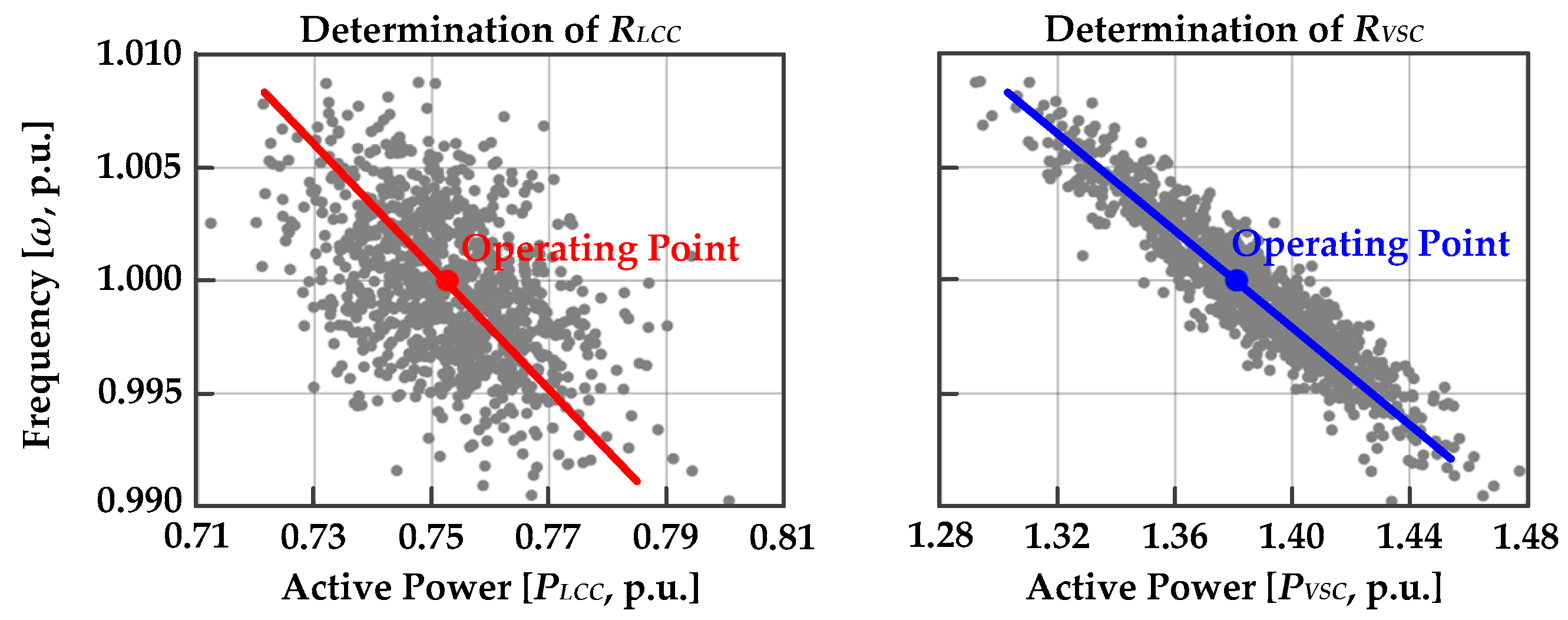
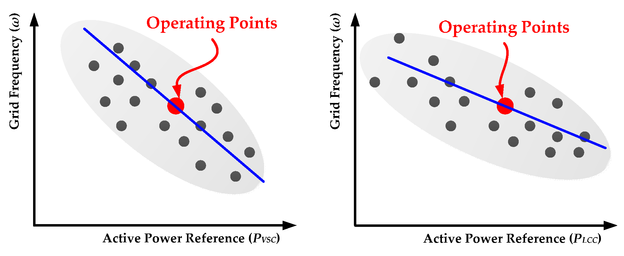
2.2.2. Graphical Analysis to Determine Droop Coefficients

In this section, we derive the droop coefficients of LCC and VSC HVDCs by graphical analysis. Figure 1 shows a concept of the proposed method of droop coefficient determination. Red points are operating points of LCC and VSC HVDCs determined by the optimization problem. Grey dots represent optimization results of the Monte Carlo samples. The points are categorized by active power reference and grid frequency, so that the frequency–power droop can be represented by the slope of the blue line, to minimize the root mean square error between the points above the blue line and the grey dots. The slopes of the blue lines are presented as −R_VSC,0 for VSC HVDC and −R_LCC,0 for the LCC HVDC. Note that the determination method is called the “graphic method”, in that curve-fitting is exploited for coefficient determination.

We can derive droop coefficients of LCC and VSC HVDCs from Figure 1, but the coefficients may not satisfy Equation (14), because the power loss of the system is not considered in (12). We can determine final values of the coefficients by the additional correction method. As active power sharing ratio of HVDCs depend on the ration of droop coefficients, final droop coefficients are corrected by multiplying the same constant to R_LCC,0 and R_VSC,0. Thus final coefficients are determined as

$$R_{VSC}(k)=\left({\displaystyle \sum _{n=1}^N\frac{R_{eq}}{R_{VSC,0}(n)}}+{\displaystyle \sum _{n=1}^N\frac{R_{eq}}{R_{LCC,0}(n)}}\right)R_{VSC,0}(k)\&R_{LCC}(k)=\left({\displaystyle \sum _{n=1}^N\frac{R_{eq}}{R_{VSC,0}(n)}}+{\displaystyle \sum _{n=1}^N\frac{R_{eq}}{R_{LCC,0}(n)}}\right)R_{LCC,0}(k),$$

(15)

where R_VSC,0(n) and R_LCC,0(n) are the coefficients of the HVDCs connected to n-th bus, derived from the graphical analysis.

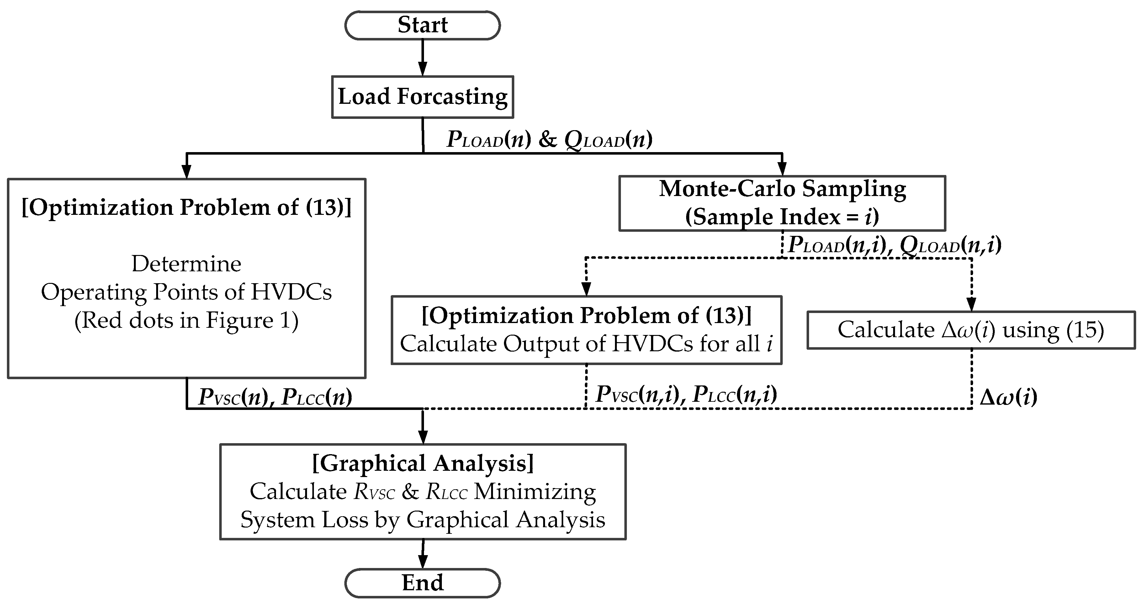
2.3. Overall Procedure

Figure 2 shows the overall procedure of the proposed method. First, the operating points of multiple HVDCs are derived from the forecasted load and scheduled output of generators using Equation (11). The Monte Carlo sampling method extracts irregular load profiles, and the active power references and frequency deviation for all samples are calculated by the samples. Note that the flow of multiple scenarios is represented by a dotted line. Finally, using the graphical approach described in Figure 1, the frequency–power droop coefficients of VSC HVDCs and LCC HVDCs are determined.

3. Simulation Results

Case studies were performed using two test systems. First, we verified the proposed method using the IEEE 14-bus test system, which is widely utilized to evaluate algorithms considering transmission networks [39]. Then, we provided the simulation results considering an actual power system, i.e., that of Jeju Island in Korea.

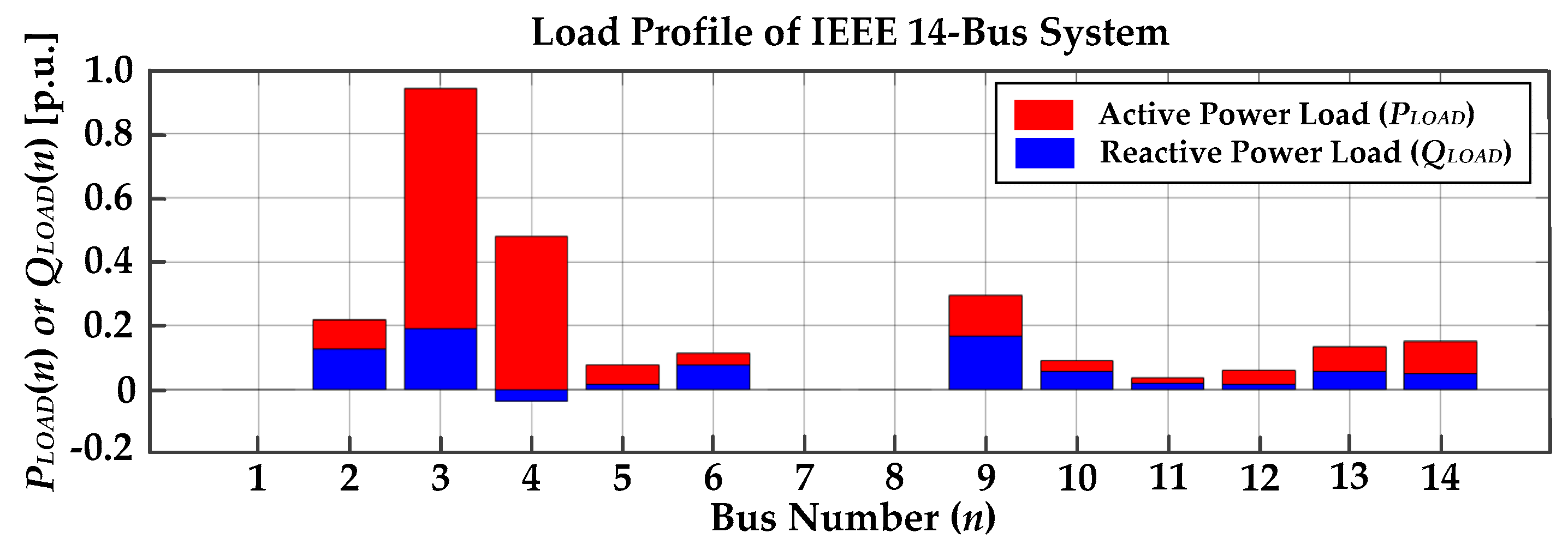
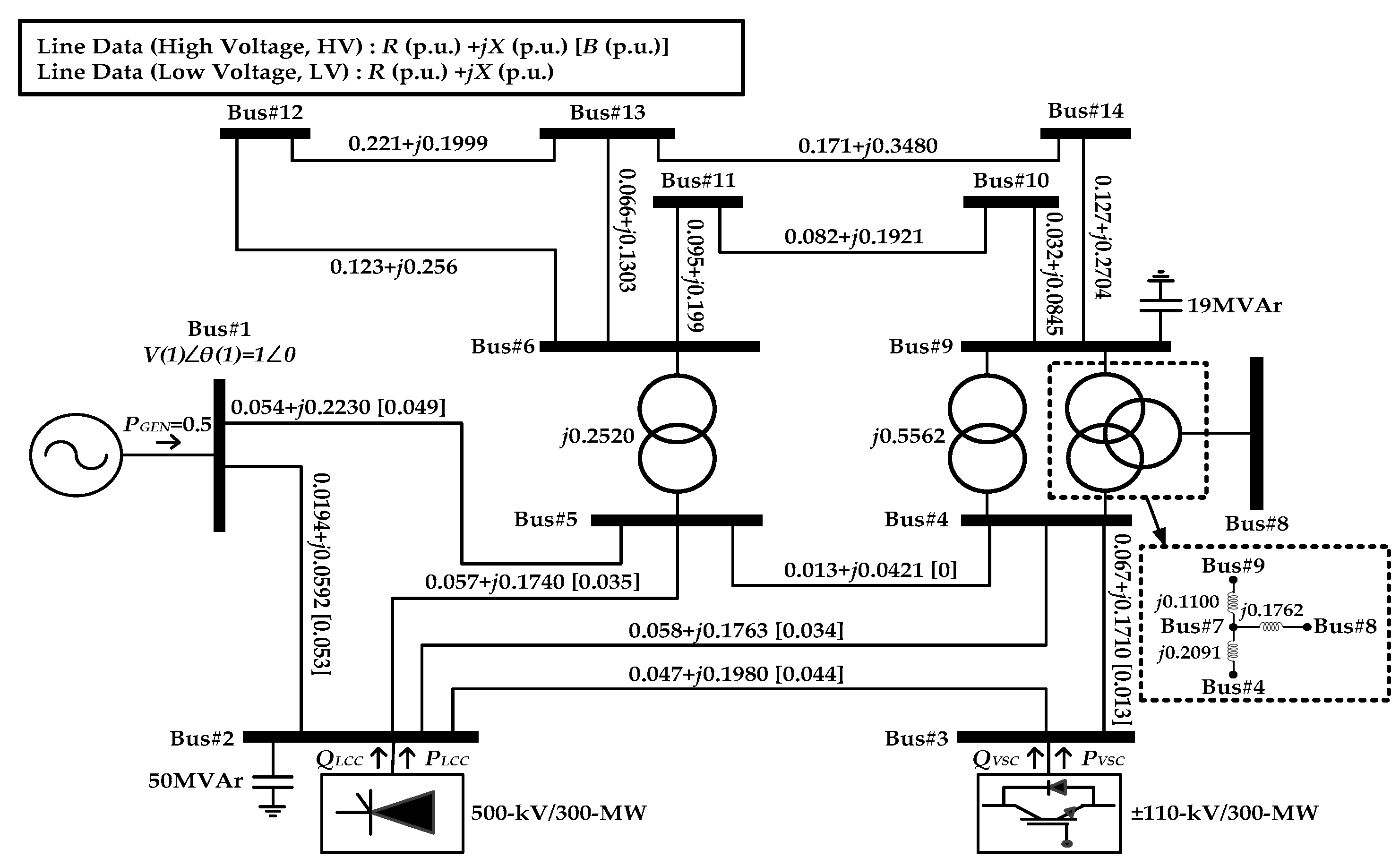
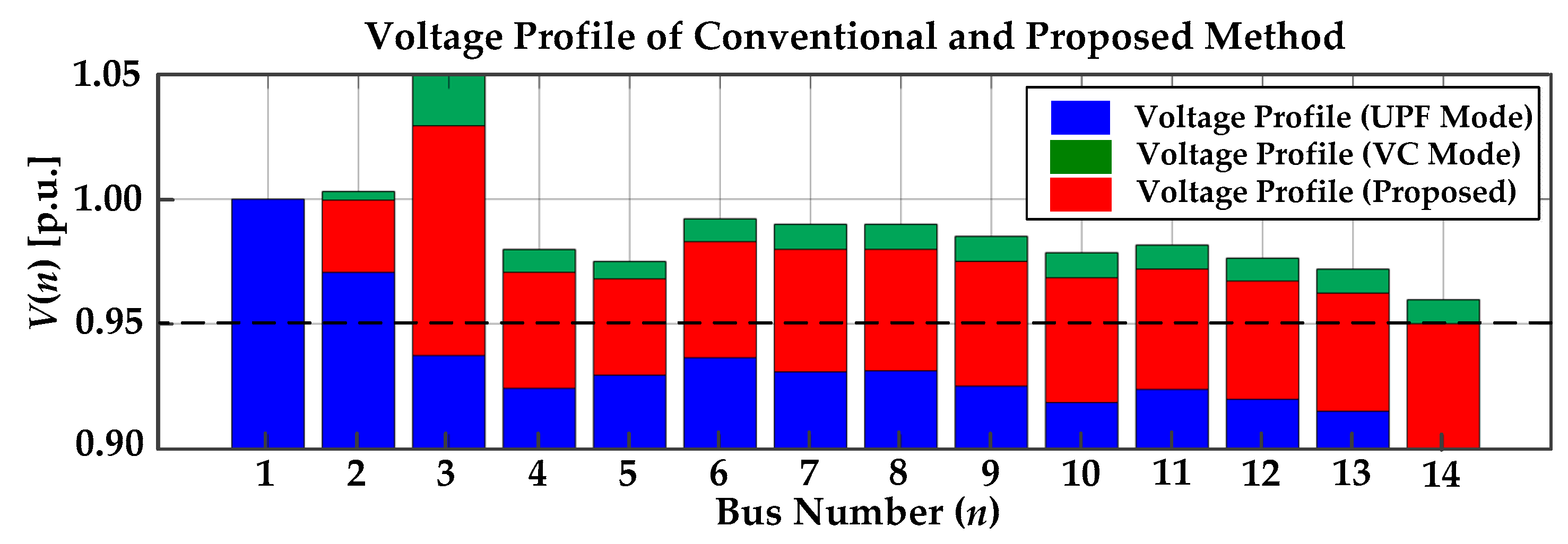
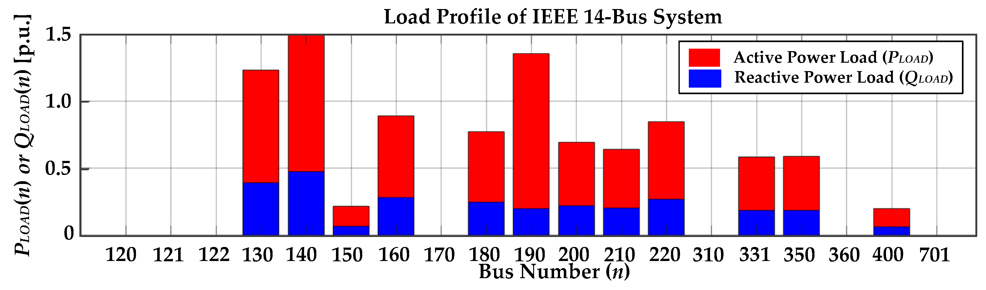
3.1. Simulation Results for the IEEE 14-Bus Test System

Figure 3 represents the modified IEEE 14-bus test system, including both LCC and VSC HVDC systems. The base of the complex power is 100 MW. Synchronous condensers are eliminated from the original test system, and only a single generator at Bus #1 is considered for simplification. Because Bus #1 is the reference bus, and the voltage-controlling generator is installed at the bus, the voltage magnitude and angle are 1 p.u. and 0 rad, respectively. The active power of the generator is fixed at 50 MW (0.5 p.u.) because it is not considered as a variable in the optimization problem. A 500 kV/200 MW LCC HVDC and a 400 kV/200 MW VSC HVDC are included at Bus #2 and #3, respectively. The parameters of the LCC HVDC are modified from the well-known CIGRE BENCHMARK model [40]. In the test system, the variables to be determined are P_LCC, P_VSC, and Q_VSC. Note that the harmonic filters and shunt capacitors of the LCC HVDC system are considered at the admittance matrix.

We compared the steady-state results of two conventional methods and the proposed method. In the first method, VSC HVDC operates in unity power factor (UPF) mode, so that the reactive power output is zero. In the second method (VC mode), the VSC HVDC controls AC voltage to be as high as possible. In both methods, the active power references of LCC and VSC HVDCs are identical. The forecasted load profile in the test system is illustrated in Figure 4, which is applied to both case studies.

Figure 5 shows voltage profiles with the conventional and proposed method. Voltage profiles are investigated in the case studies, in that security constraints of AC voltage should be satisfied by utilizing the optimization problem. In UPF mode, the AC voltage profiles of most buses are lower than the lower bound (V_lb), as shown by the blue areas of Figure 5. On the other hand, in VC mode, AC voltage is maintained within the operational boundaries, because VSC HVDC compensates reactive power into the network as much as possible. The voltage is also maintained within its boundaries using the proposed method, because constraints on AC voltage are reflected in the optimization problem. However, the amount of reactive power with the proposed method is smaller than that of the VC mode, as shown in Figure 5.

Table 1. Comparison of power in three cases.

	UPF Mode	VC Mode	Proposed
Output of LCC HVDC (PLCC)	112.02 MW	111.96 MW	84.08 MW
Output of VSC HVDC (PVSC)	112.02 MW	111.96 MW	139.26 MW
Power loss	5.04 MW	4.92 MW	4.34 MW

UPF: unity power factor, VC: voltage control.

shows the comparisons of active power outputs of LCC and VSC HVDCs, and the resulting power loss in three cases. As the outputs of LCC and VSC HVDCs are intended to be identical in the conventional methods, both HVDCs provide the same active power into the power network. On the other hand, VSC HVDC provides more active power than LCC HVDC in the case of the proposed method to minimize system loss. As a result, the active power loss of the test system with the proposed method is reduced 13.89% and 11.79% from that of the UPF mode and VC mode, respectively. Even the voltage level is higher when VSC HVDC operates on VC mode than the proposed case; power loss is smaller when using the proposed method, because the current flow increases for reactive power compensation in VC mode. As shown in Figure 5 and Table 1, the simulation results suggest that the proposed method is effective with steady-state characteristics for the IEEE 14-bus test system.

To verify the droop coefficient determination method, we generate 10,000 load profiles reflecting forecasting error. We assume that the active and reactive load profile follows the normal distribution function, in which the average is the forecasted value and the standard deviation is 3% of the forecasted value. According to a previous study [21], we define R_eq and D as 0.1 and 2, respectively. Figure 6 illustrates the graphical analysis of the frequency–power droop coefficient design methodology. As the optimization results are scattered as grey dots in Figure 6, we can define the droop coefficients of LCC and VSC HVDCs—R_LCC and R_VSC, respectively—like their corresponding lines.

Using Equation (15), we can derive the final droop coefficient values as R_LCC = 0.227 and R_VSC = 0.179. The calculated droop coefficients are verified by comparison with the conventional case. The conventional case is defined as the situation where the operating points are determined by the optimization, and the droop coefficients are determined proportional to their capacity [41]. To verify the proposed determination method, we utilized 10 randomly sampled load profiles.

Table 2. Comparison of power loss between randomly sampled load profiles.

	Conventional	Proposed
Deviation of LCC HVDC’s output (ΔPLCC)	−0.32 MW	−0.28 MW
Deviation of VSC HVDC’s output (ΔPVSC)	−0.32 MW	−0.35 MW
Deviation of power loss	−36.41 kW	−36.74 kW

shows the comparison of average outputs and power losses. As described in Table 2, the deviation of power loss increased using the proposed method to reduce total system loss. From the simulation results in Table 1 and Table 2, we suggest that the proposed optimization problem and the droop coefficient determination method enhance the efficiency of the test system.

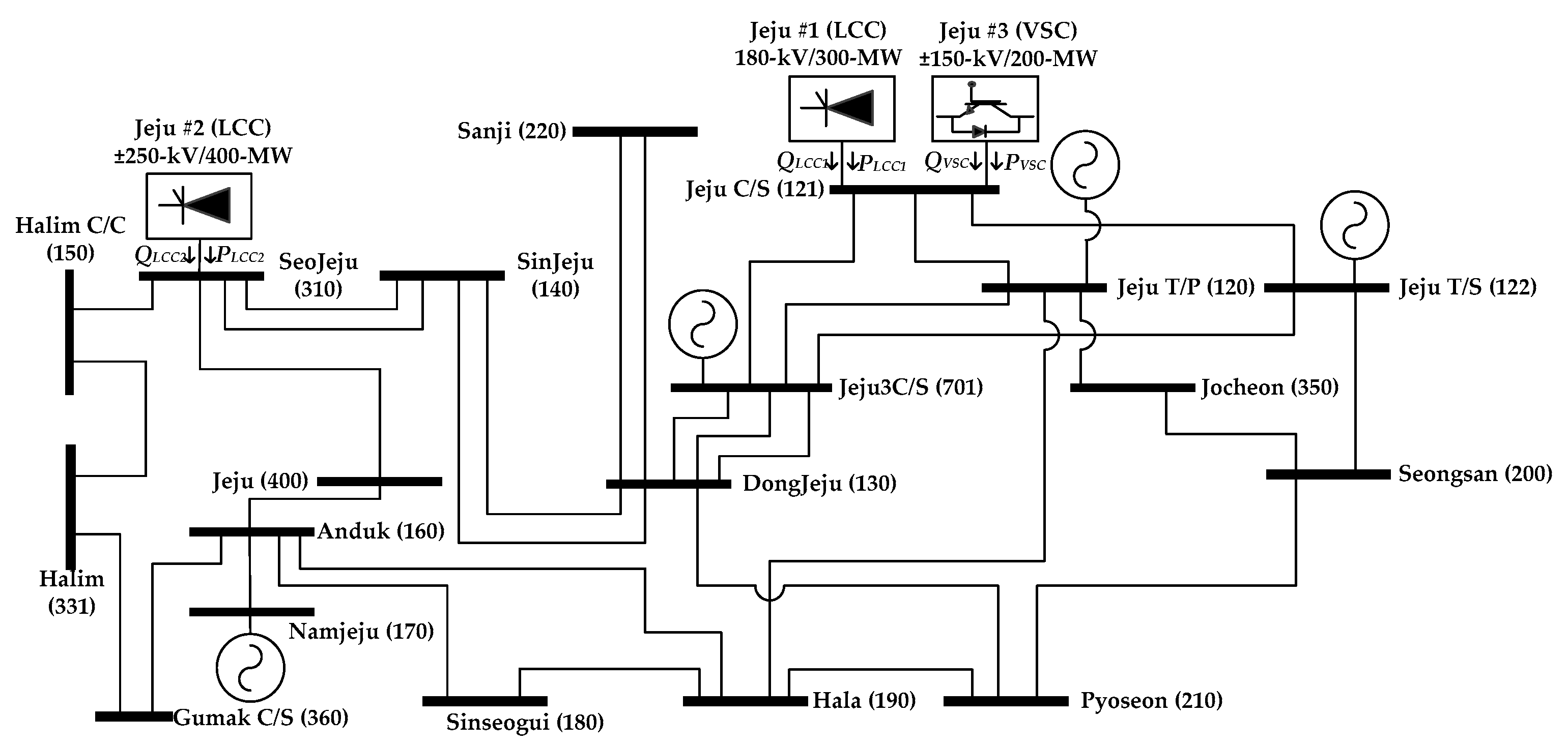
3.2. Simulation Results for the Jeju Island System

Figure 7 shows the configuration of the Jeju Island power network [42]. There are four generators and three HVDC systems, i.e., two LCC HVDCs and one VSC HVDC. The first LCC HVDC is a 180 kV/300 MW system constructed in 1998, and the second LCC HVDC is a ±250 kV/400 MW system constructed in 2013. The VSC HVDC considered in the simulation is a planned installation with a capacity of ±150 kV/200 MW. The base of complex power is 100 MW, and the base voltage is 154 kV. The active power of generators, line impedance, and data of the shunt compensator in the test system are represented in Appendix A. The actual load data from Jeju Island at peak time is utilized, as illustrated in Figure 8. The simulation scenarios are similar to those with the IEEE 14-bus test system. Only one generator at Jeju 3C/S controls the voltage magnitude at 1.04 p.u., and the other generators only regulate active power, which means that the reactive power of these generators is zero. The output of the conventional method is determined proportional to capacity.

Table 3. Comparison of power loss between the conventional and proposed methods.

	Conventional	Proposed
Output of Jeju #1 (PLCC1)	132.82 MW	50.17 MW
Output of Jeju #2 (PLCC2)	177.09 MW	305.73 MW
Output of Jeju #3 (PVSC)	88.55 MW	41.80 MW
Power loss	6.26 MW	5.50 MW

shows the results of steady-state analysis using the conventional and proposed methods. As the outputs of multiple HVDCs are determined proportional to their capacity in the conventional method, the active power ratio of Jeju #1, #2, and #3 is 3:4:2. On the other hand, the results of the proposed method determine the operating points of the HVDCs using an optimization problem. Thus, power loss in the system was reduced 13.82% from that of the conventional method. The results suggest that operation with the proposed optimization problem would reduce power loss. In the second case, Jeju #1 and Jeju #3 are connected to same bus. Among two HVDC systems, the ratio of active power is not significant, because they are connected to same bus. However, the references to them are determined because LCC HVDC absorbs reactive power different from the VSC HVDC. Therefore, the proposed optimization problem considers not only active power but also optimal reactive power flow.

Figure 9 presents a graphical analysis of droop coefficient determination. To verify the droop coefficient determination method, 1000 randomly extracted scenarios were utilized. Equivalent droop coefficients R_eq and D were assumed to be identical to the previous case study. As a result, we could derive the droop coefficients, R_LCC1, R_LCC2, and R_VSC, as 0.298, 0.233, and 0.426, respectively.

The droop coefficients derived from Figure 9 are verified by comparison with the conventional case, in which the steady-state system is determined by an optimization problem. The only difference between the conventional and proposed methods is that the droop coefficients are proportional to capacity in the conventional method.

Table 4. Comparisons of average power loss deviation for irregular load profiles.

	Conventional	Proposed
Deviation of power loss	1.683 kW	1.675 kW

shows the average loss deviation from the power loss at steady-state for 1000 random cases. Power loss deviation is reduced 0.48% using the proposed droop coefficients. The difference is very small because the droop coefficient in the conventional method is very similar to that of the proposed method; however, the power loss is successfully reduced using the proposed method.

4. Conclusions

We propose the use of an optimization problem for MIDC systems. The optimization problem considers both the LCC and VSC HVDCs, and we derived their models to analyze the efficiency of the AC network. The purpose of the problem is loss minimization. Furthermore, we utilized the optimization problem to determine the frequency–power droop coefficients of multiple HVDCs, considering characteristics of both the LCC and VSC HVDCs. The determination method calculates the coefficients by minimizing the root mean square error between the numerous optimization results from the Monte Carlo sampling method, asw well as the linear-approximated values. As several small optimization problems are solved in the proposed method rather than one big problem, the proposed method reduces computation burdens compared with conventional stochastic optimization problems. In other words, the computation time increases arithmetically with the number of samples for our method. Two test systems, an IEEE 14-bus test system and an actual Jeju grid, were used to verify the proposed method. From the simulation results, we suggest that the proposed method efficiently reduces loss in the power system. For future work, consideration of an overall system, including HVDC networks and an AC system for the sending side, is required. By investigating the overall system using the proposed method, we can find globally optimized operating points of multiple HVDC systems, in order to enhance power system efficiency.

References

1. Figueroa-Acevedo, A.L.; Czahor, M.S.; Jahn, D.E. A comparison of the technological, economic, public policy, and environmental factors of HVDC and HVAC interregional transmission. AIMS Energy 2015, 3, 144–161. [Google Scholar] [CrossRef]
2. Li, B.; Liu, T.; Xu, W.; Li, Q.; Zhang, Y.; Li, Y.; Li, X.Y. Research on technical requirements of line-commutated converter-based high-voltage direct current participating in receiving end AC system’s black start. IET Gener. Transm. Distrib. 2016, 10, 2071–2078. [Google Scholar] [CrossRef]
3. Wang, L.; Thi, M.S. Stability enhancement of a PMSG-based offshore wind farm fed to a multi-machine system through LCC-HVDC link. IEEE Trans. Power Syst. 2013, 28, 3327–3334. [Google Scholar] [CrossRef]
4. Bidadfar, A.; Nee, H.; Zhang, L.; Harnefors, L.; Namayantavana, S.; Abedi, M.; Karrari, M.; Gharehpetian, G.B. Power system stability analysis using feedback control system modeling including HVDC transmission links. IEEE Trans. Power Syst. 2016, 31, 116–124. [Google Scholar] [CrossRef]
5. Azad, S.P.; Taylor, J.A.; Iravani, R. Decentralized supplementary control of multiple LCC-HVDC links. IEEE Trans. Power Syst. 2016, 31, 572–580. [Google Scholar] [CrossRef]
6. Azad, S.P.; Iravani, R.; Tate, J.E. Stability enhancement of a DC-segmented AC power system. IEEE Trans. Power Deliv. 2015, 30, 737–745. [Google Scholar] [CrossRef]
7. Kwon, D.; Kim, Y.; Moon, S. Modeling and Analysis of an LCC HVDC system using DC voltage control to improve transient response and short-term power transfer capability. IEEE Trans. Power Deliv. 2018, 33, 1922–1933. [Google Scholar] [CrossRef]
8. Zhang, M.; Yuan, X.; Hu, J. Inertia and primary frequency provisions of PLL-synchronized VSC HVDC when attached to islanded AC system. IEEE Trans. Power Syst. 2018, 33, 4179–4188. [Google Scholar] [CrossRef]
9. Jang, G.; Oh, S.; Han, B.M.; Kim, C.K. Novel reactive power compensation scheme for the Jeju-Haenam HVDC system. IEE Proc.-Gener. Transm. Ditrib. 2005, 152, 514–520. [Google Scholar] [CrossRef]
10. Market, P.E.; Skliutas, J.P.; Sung, P.Y.; Kim, K.S.; Kim, H.M.; Sailer, L.H.; Young, R.R. New synchronous condensers for Jeju island. In Proceedings of the 2012 IEEE Power & Energy Society General Meeting, San Diego, CA, USA, 22–26 July 2012. [Google Scholar]
11. Yoon, M.; Yoon, Y.; Jang, G. A study on maximum wind power penetration limit in island power system considering high-voltage direct current interconnections. Energies 2015, 8, 14244–14259. [Google Scholar] [CrossRef]
12. Davies, B.; Williamson, A.; Gole, A.M.; Ek, B.; Long, B.; Burton, B.; Kell, D.; Brandt, D.; Lee, D.; Rahimi, E.; et al. Systems with multipld DC infeed. In CIGRE Working Group B4.41; CIGRE: Paris, France, 2008. [Google Scholar]
13. Gui, C.; Zhang, Y.; Gole, A.M.; Zhao, C. Analysis of dual-infeed HVDC with LCC-HVDC and VSC-HVDC. IEEE Trans. Power Deliv. 2012, 27, 1529–1597. [Google Scholar] [CrossRef]
14. Ni, X.; Gole, A.M.; Zhoa, C.; Guo, C. An improved measure of AC system strength for performance analysis of multi-infeed HVdc systems including VSC and LCC converters. IEEE Trans. Power Deliv. 2018, 33, 169–178. [Google Scholar] [CrossRef]
15. Rahimi, E.; Gole, A.M.; Davies, J.B.; Fernando, I.T.; Kent, K.L. Commutation failure analysis in multi-infeed HVDC systems. IEEE Trans. Power Deliv. 2011, 26, 378–384. [Google Scholar] [CrossRef]
16. Hwang, S.; Lee, J.; Jang, G. HVDC-system-interaction assessment through line flow change distribution factor and transient stability analysis at planning stage. Energies 2016, 9, 1068. [Google Scholar] [CrossRef]
17. Rabiee, A.; Soroudi, A.; Keane, A. Information gap decision theory based OPF with HVDC connected wind farms. IEEE Trans. Power Syst. 2015, 30, 3396–3406. [Google Scholar] [CrossRef]
18. Pizano-Martinez, A.; Fuerte-Esquivel, C.R.; Ambriz-Perez, H.; Acha, E. Modeling of VSC-based HVDC systems for a Newton-Raphson OPF algorithm. IEEE Trans. Power Syst. 2007, 22, 1794–1803. [Google Scholar] [CrossRef]
19. Gavriluta, C.; Candela, I.; Luna, A.; Gomez-Exposito, A.; Rodriguez, P. Hierarchical control of HV-MTDC systems with droop-based primary and OPF-based secondary. IEEE Trans. Smart Grid 2015, 6, 1502–1510. [Google Scholar] [CrossRef]
20. Han, M.; Xu, D.; Wan, L. Hierarchical optimal power flow control for loss minimization in hybrid multi-terminal HVDC transmission system. CSEE J. Power Energy Syst. 2016, 2, 40–46. [Google Scholar] [CrossRef]
21. Kundur, P.; Balu, N.J.; Lauby, M.G. Power System Stability and Control; McGraw-Hill: New York, NY, USA, 1994. [Google Scholar]
22. Liu, H.; Chen, Z. Contribution of VSC-HVDC to frequency regulation of power systems with offshore wind generation. IEEE Trans. Energy Convers. 2015, 30, 918–926. [Google Scholar] [CrossRef]
23. Adeuyi, O.D.; Cheah-Mane, M.; Liang, J.; Jenkins, N. Fast frequency response from offshore multiterminal VSC-HVDC schemes. IEEE Trans. Power Deliv. 2017, 32, 2442–2452. [Google Scholar] [CrossRef]
24. Kwon, D.; Kim, Y.; Moon, S.; Kim, C. Modeling of HVDC system to improve estimation of transient DC current and voltages for AC line-to-ground fault-an actual case study in Korea. Energies 2017, 10, 1543. [Google Scholar] [CrossRef]
25. Abdel-Khalik, A.S.; Massoud, A.M.; Elserougi, A.A.; Ahmed, S. Optimum power transmission-based droop control design for multi-terminal HVDC of offshore wind farm. IEEE Trans. Power Syst. 2013, 28, 3401–3409. [Google Scholar] [CrossRef]
26. Agundis-Tinajero, G.; Diaz, N.L.; Luna, A.C.; Segundo-Ramírez, J.; Visairo-Cruz, N.; Gerrero, J.M.; Vazquez, J.C. Extended-optimal-power-flow-based hierarchical control for islanded AC microgrids. IEEE Trans. Power Electron. 2018, 34, 840–848. [Google Scholar] [CrossRef]
27. Cao, J.; Du, W.; Wang, H.F.; Bu, S.Q. Minimization of transmission loss in meshed AC/DC grids with VSC-MTDC networks. IEEE Trans. Power Syst. 2013, 28, 3047–3055. [Google Scholar] [CrossRef]
28. Flourentzou, N.; Agelidis, V.G.; Demetriades, G.D. VSC-based HVDC power transmission systems: An overview. IEEE Trans. Power Electron. 2009, 24, 592–602. [Google Scholar] [CrossRef]
29. Li, Y.; Luo, L.; Rehtanz, C.; Rüberg, S.; Liu, F. Realization of reactive power compensation near the LCC-HVDC converter bridges by means of an inductive filtering method. IEEE Trans. Power Electron. 2009, 24, 592–602. [Google Scholar] [CrossRef]
30. He, X.; Geng, H.; Yang, G.; Zou, X. Coordinated Control for Large-Scale Wind Farms with LCC-HVDC Integration. Energies 2018, 11, 2207. [Google Scholar] [CrossRef]
31. DJesus, M.E.M.; Martin, D.S.; Arnaltes, S.; Castronuovo, E.D. Optimal operation of offshore wind farms with line-commutated HVDC link connection. IEEE Trans. Energy Convers. 2010, 25, 504–513. [Google Scholar] [CrossRef]
32. Bergen, A.R.; Vittal, V. Power Systems Analysis, 2nd ed.; Prentice-Hall: Upper Sandle River, NJ, USA, 1994. [Google Scholar]
33. Sahli, Z.; Hamouda, A.; Bekrar, A.; Trentesaux, D. Reactive Power Dispatch Optimization with Voltage Profile Improvement Using an Efficient Hybrid Algorithm. Energies 2018, 11, 2134. [Google Scholar] [CrossRef]
34. Jeong, M.G.; Kim, Y.J.; Moon, S.I.; Hwang, P.I. Optimal voltage control using an equivalent model of a low-voltage network accommodating inverter-interfaced distributed generators. Energies 2017, 10, 1180. [Google Scholar] [CrossRef]
35. Huang, Y.; Yang, K.; Zhang, W.; Lee, K.Y. Hierarchical energy management for the multienergy carriers system with different interest bodies. Energies 2018, 11, 2834. [Google Scholar] [CrossRef]
36. Li, J.; Wang, B.; Ren, H.; Zhao, D.; Wang, F.; Shafie-khah, M.; Catalāo, J.P.S. Two-tier reactive power and voltage control strategy based on ARMA renewable power forecasting models. Energies 2017, 10, 1518. [Google Scholar]
37. Yuan, C.; Xie, P.; Yang, D.; Xiao, X. Transient stability analysis of islanded AC microgrids with a significant share of virtual synchronous generators. Energies 2018, 11, 44. [Google Scholar] [CrossRef]
38. Sauhats, A.; Zemite, L.; Petrichenko, L.; Moshkin, I.; Jasevics, A. Estimating the economic impacts of net metering schemes for residential PV systems with profiling of power demand, generation, and market prices. Energies 2018, 11, 3222. [Google Scholar] [CrossRef]
39. Modeling and Simulation of IEEE 14 Bus System with FACTS Controllers; Electrical and Computer Engineering Department, University of Waterloo: Waterloo, ON, Canada, 2003; Available online: https://www.researchgate.net/profile/Mohamed_Mourad_Lafifi/post/Datasheet_for_5_machine_14_bus_ieee_system2/attachment/59d637fe79197b8077995408/AS%3A395594351824896%401471328451959/download/MODELING+AND+SIMULATION+OF+IEEE+14+BUS+SYSTEM+WITH+FACTS+CONTROLLERS+IEEEBenchmarkTFreport.pdf (accessed on 11 February 2019).
40. Faruque, M.O.; Zhang, Y.; Dinavahi, V. Detailed modeling of CIGRE HVDC benchmark system using PSCAD/EMTDC and PSB/SIMULINK. IEEE Trans. Power Deliv. 2005, 21, 378–387. [Google Scholar] [CrossRef]
41. Mohamed, Y.A.-R.I.; El-Saadany, E.F. Adaptive decentralized droop controller to preserve power sharing stability of paralleled inverters in distributed generation microgrids. IEEE Trans. Power Electron. 2008, 23, 2806–2816. [Google Scholar] [CrossRef]
42. An, K.; Song, K.B.; Hur, K. Incorporating charging/discharging strategy of electric vehicles into security-constrained optimal power flow to support high renewable penetration. Energies 2017, 10, 729. [Google Scholar] [CrossRef]
Figure 1. Concept of the method to determine frequency–power droop coefficients of voltage sourced converter (VSC) and line commutated converter (LCC) high-voltage direct currents (HVDCs).
Applsci 09 00606 g001
Figure 2. Overall procedure of the proposed method to calculate droop coefficients.
Applsci 09 00606 g002
Figure 3. Configuration of Institute of Electrical and Electronics Engineers (IEEE) 14-bus test system.
Applsci 09 00606 g003
Figure 4. Forecasted load profile for the IEEE 14-bus test system.
Applsci 09 00606 g004
Figure 5. Voltage profile of the conventional and proposed methods in the IEEE 14-bus test system.
Applsci 09 00606 g005
Figure 6. Graphical coefficient determination method applied to the IEEE 14-bus test system.
Applsci 09 00606 g006
Figure 7. Configuration of the Jeju Island network with multiple HVDCs.
Applsci 09 00606 g007
Figure 8. Load profile for Jeju Island.
Applsci 09 00606 g008
Figure 9. Graphical analysis of the coefficient determination method applied to the Jeju Island system.
Applsci 09 00606 g009