Numerical Study on Dynamic-Stall Characteristics of Finite Wing and Rotor

Abstract

To study the three-dimensional effects on the dynamic-stall characteristics of a rotor blade, the unsteady flowfields of the finite wing and rotor were simulated under dynamic-stall conditions, respectively. Unsteady Reynolds-averaged Navier–Stokes (URANS) equations coupled with a third-order Roe–MUSCL spatial discretization scheme were chosen as the governing equations to predict the three-dimensional flowfields. It is indicated from the simulated results of a finite wing that dynamic stall would be restricted near the wing tip due to the influence of the wing-tip vortex. By comparing the simulated results of the finite wing with the spanwise flow, it is indicated that the spanwise flow would arouse vortex accumulation. Consequently, the dynamic stall is restricted near the wing root and aggravated near the wing tip. By comparing the simulated results of a rotor in forward flight, it is indicated that the dynamic stall of the rotor would be inhibited due to the effects of the spanwise flow and Coriolis force. This work fills the gap regarding the insufficient three-dimensional dynamic stall of a helicopter rotor, and could be used to guide rotor airfoil shape design in the future.

1. Introduction

To satisfy the flight requirements of a helicopter in forward flight, rotor blades are designed to perform pitching, flapping, and rotation movements. Therefore, rotor blades work in unsteady aerodynamic environments compared with a fixed-wing aircraft. As a result, the aerodynamic characteristics of helicopter rotor are much more complex, and the dynamic-stall phenomenon [1,2] usually occurs on the rotor blades of a helicopter in forward flight. Consequently, many negative influences, such as stall flutter and vibration and noise increase could arise due to dynamic-stall effects. Therefore, dynamic-stall characteristics have significant influence on the aerodynamics performance of a helicopter. Hence, studies for improving aerodynamic rotor performance would directly face the dynamic-stall phenomenon. As a result, investigations of the dynamic-stall phenomenon have received considerable attention in recent years.

Aiming to develop a full understanding of rotor dynamic-stall characteristics, many investigations on two-dimensional (2D) rotor airfoil dynamic stall were done in the last 40 years to reveal the physical characteristics of this phenomenon, including experimental [3,4,5], theoretical [6,7], and numerical methods [8,9,10]. However, the dynamic-stall characteristics of an airfoil are obviously different from those of a rotor. As a result, some studies on the three-dimensional (3D) dynamic-stall characteristics of a finite wing or rotor were done by employing experiment and numerical methods. Horner [11] researched the 3D flow structures that arise from 2D airfoil/wall interactions by using the smoke-wire visual method, and a simple vortex image model was established to describe the 3D vortex structures of the dynamic stall. Lorber [12] also performed an experiment to investigate the dynamic-stall characteristics of a 3D wing. The test results indicated that the wing-tip vortex could delay dynamic stall due to the reduction of the effective angle of attack (AoA) for an unswept wing. Interaction between the tip vortex and wing was reduced for a swept wing. Later, by using Particle Image Velocimetry (PIV) technology, Mulleners [13] measured the 3D flowfield of a fully equipped helicopter model. The measured results revealed that a large-scale dynamic-stall vortex appeared at a 50%–60% radius on the retreating blade, and rotor rotation would have a stabilizing effect on the formation and convection of the dynamic-stall vortex. Raghav [14,15,16] investigated the 3D flowfield over a retreating blade by using the Stereoscopic Particle Image Velocimetry method under a dynamic-stall condition. This research demonstrated that centrifugal effects played a strong role on radial flow in the separated flow regions, and affected dynamic-stall vortex formation. Recently, Raffel [17] performed a new experiment by employing the Differential Infrared Thermography (DIF) method to investigate the dynamic-stall characteristics of a rotor. This study indicated that the DIF method could differentiate the stalled and attached flow with no contacted-blade surface treatment. Merz [18] investigated the dynamic-stall characteristics of a rotor blade with parabolic-tip geometry. The experiment results indicated that the tip vortex could reduce the lift near the blade tip under a static condition. However, the lift remained higher, near the blade tip, under the dynamic-stall condition due to the influence of vorticity accumulation.

With the development of computer technology, the computational fluid dynamics (CFD) method has the advantages of less time consumption and lower cost compared with the experimental methods. Therefore, the numerical method was widely used in 3D dynamic-stall studies. By employing CFD, a numerical study about the 3D dynamic stall of a wing with an NACA0015 airfoil was performed by Salari [19]. It was indicated that wind sweep could delay dynamic-stall vortex formation and decrease aerodynamic force peaks compared with a 2D condition. In 1995, Ekaterinaris [20] developed an upwind-biased iterative-flow solver to investigate an unsteady 3D flowfield over an oscillating wing. Spentzos [21] researched the 3D dynamic-stall characteristics of a wing by using the CFD method. Numerical results indicated that an Ω-topology vortex formed due to the interaction of the wing-tip vortex and dynamic-stall vortex. It was also illustrated that the geometry of the tip had significant influence on the dynamic-stall characteristics. Raghav [22] investigated the dynamic-stall characteristics of a rotor in forward flight by employing an experimental and a computational method, and this research captured the radial-jet layer caused by radial acceleration. In 2012, Gardner [9] conducted a rotational-effect investigation on deep dynamic stall by using CFD. The numerical results illustrated that rotational effects can reduce aerodynamic-load peaks and cause earlier airflow reattachment. Later, Kaufmann [23] simulated the dynamic-stall phenomenon on an oscillating finite wing. The numerical results were in good agreement with the experimental results, and revealed an Ω-shape vortex. Costes [24] simulated the dynamic-stall characteristics of a finite wing by employing CFD. It was indicated that the numerical method could correctly capture the physical characteristics of dynamic stall. Jain [25] also investigated the dynamic stall of a finite-span wing by employing NASA’s OVERFLOW flow solver and ONERA’s elsA flow solver. The numerical results indicated that the transition model could improve static-angle prediction, but it could also lead to separated-flow overpredictions. Recently, Visbal [26] performed an investigation on the spanwise end effects on the dynamic stall of a finite wing. It was illustrated in this study that spanwise end and aspect ratio can both significantly affect the dynamic-stall flow structure.

However, the influence of spanwise flow on the dynamic-stall vortex was seldom considered in previous studies. As a result, some dynamic-stall potential problems of a rotor still exist due to the 3D effects. In order to obtain a deeper understanding of these 3D effects on dynamic stall, the unsteady aerodynamic characteristics of a finite wing are studied under spanwise flow and nonspanwise flow by using the URANS CFD method. A study on unsteady aerodynamic characteristics of a rotor in forward flight was also performed.

2. Numerical Methods

2.1. Grid Generational Method

C-topology grids around a 2D airfoil are calculated in this research by solving the Poisson equations. Based on 2D airfoil grids, finite-wing grids, and rotor-blade grids (359 × 60 × 100) with C-O topology are generated by interpolating, folding, and deforming. Cartesian grids (120 × 120 × 120) are used as background grids in this study. In order to capture the unsteady vortex, background grids are properly refined. The Hole Map and Inverse Map methods [27] were employed to identify the boundary cells of the hole and the donor elements, respectively. The schematic diagram of the finite wing in background grids is shown in Figure 1, where z represents a nondimensional spanwise position ($z=r/R$) of the finite wing and rotor blade, and r and R represent the physical position and length of the wing/blade, respectively. The wing/blade with an aspect ratio of 10.0 was composed with a classical NACA0012 airfoil in this research.

2.2. Flowfield Solver Method

The Navier–Stokes (N–S) equations employed in this research can be expressed as:

$$\frac{\partial }{\partial t}{\displaystyle \underset{\Omega }{\iiint }Wd\Omega }+{\displaystyle \underset{\partial \Omega }{\iint }(F_c}-F_v)dS=0$$

(1)

where, $W$ denotes conserved variables, $F_c$ represents convective fluxes, and $F_v$ represents viscous fluxes, i.e.,

$$W=\left[\begin{array}{c}\rho \\ \rho u\\ \rho v\\ \rho w\\ \rho E\end{array}\right],F_c=\left[\begin{array}{c}\rho V_r\\ \rho u{V}_r+n_{x}p\\ \rho v{V}_r+n_{y}p\\ \rho w{V}_r+n_{z}p\\ \rho H{V}_r+V_{t}p\end{array}\right],F_v=\left[\begin{array}{c}0\\ n_x{\tau }_{xx}+n_y{\tau }_{xy}+n_z{\tau }_{xz}\\ n_x{\tau }_{yx}+n_y{\tau }_{yy}+n_z{\tau }_{yz}\\ n_x{\tau }_{zx}+n_y{\tau }_{zy}+n_z{\tau }_{zz}\\ n_x{\Theta }_x+n_y{\Theta }_y+n_z{\Theta }_z\end{array}\right]$$

(2)

where,$V_r=V-V_c$ ($V_c$ represents contravariant velocity). Symbols $\rho$,$p$, and $E$ represent the density, static pressure, and total airflow energy, respectively. ${\tau }_{ij}$ represents viscous stresses, $n_i$ represents the unit normal vector, and ${\Theta }_i$ describes viscous airflow stresses.

Aiming at predicting the unsteady flowfield of the finite wing and rotor, temporal discretization of the N–S equations is accomplished by employing the dual time-stepping approach, which can be written as:

$$\frac{3W^{n+1}-4W^n+W^{n-1}}{2\Delta t}+R(W^{n+1})=0$$

(3)

where $\Delta t$ represents the global physical time step, and $R$ represents the residual one.

In order to improve computational efficiency, the implicit LU-SGS scheme was employed in this study. The LU-SGS scheme is based on the factorization of the implicit operator into the following three parts:

$$(D+L)D^{-1}(D+U)\Delta W^n=-R^n$$

(4)

where, L is a strictly lower triangular matrix, U is a strictly upper triangular matrix, and D is a diagonal term. Based on this discretization, the LU-SGS scheme is solved by two steps, a forward and a backward sweep, i.e.,

$$\begin{array}{l}(D+L)\Delta W^{(1)}=-R^n\\ (D+U)\Delta W^{(n)}=D\Delta W^{(1)}\end{array}$$

(5)

where, $W^{n+1}=W^n+\Delta W^n$.

To accurately predict the unsteady aerodynamic characteristics of a vortical flowfield, the Roe method [28], coupled with a third-order MUSCL scheme, was employed to accomplish spatial discretization. In addition, the one-equation Spalart-Allmaras (S-A) turbulence model [29] was employed to close the N–S equations.

2.3. Flowfield-Solver Verification

In order to verify the accuracy of the CFD method employed in this research, the comparisons of the simulated lift coefficient (C_l) of the NACA00112 airfoil (2D) and the finite wing (3D) with test data [30] under a dynamic-stall condition are shown in Figure 2. In this case, the Mach number (Ma) was 0.286, reduced frequency (k) as 0.151, and the AoA was $\alpha ={14.91}^{\circ }-{9.88}^{\circ }\sin (\omega t)$, where $\omega$ represents angular velocity. It can be seen that the numerical results of the 2D airfoil were well-correlated with the test data. However, the numerical results of the finite wing had a larger stall angle and the maximum C_l compared with the 2D numerical results due to the influence of the three-dimensional effect.

Another comparison of numerical normal force coefficient C_n of the SA349/2 rotor with the test data [31], at an advance ratio of 0.26, is shown in Figure 3; $\psi$ represents the azimuthal angle of rotor blade. It is illustrated that the numerical data were also in agreement with the test data at a blade section of r/R = 0.75. Therefore, it is indicated that the present CFD method could effectively simulate the aerodynamic characteristics of a finite wing and rotor under dynamic-stall conditions.

3. Analyses and Discussion

The dynamic-stall characteristics of a rotor would be influenced by spanwise flow, blade-tip vortex, and blade rotation. As a result, in order to clearly investigate the 3D effects on dynamic-stall characteristics, we decouple the influence factors of the 3D effects into three parts. First, the dynamic-stall characteristics of a finite wing were investigated to explore the influence of the wing-tip vortex on the characteristics. Second, the dynamic-stall characteristics of a finite wing with spanwise flow were investigated to explore the influence of the flow on the characteristics. Finally, the dynamic-stall characteristics of a rotor were investigated in forward flight to explore the synthetic influence of the vortex, spanwise flow, and blade rotation.

3.1. Finite-Wing Dynamic Stall with Nonspanwise Flow

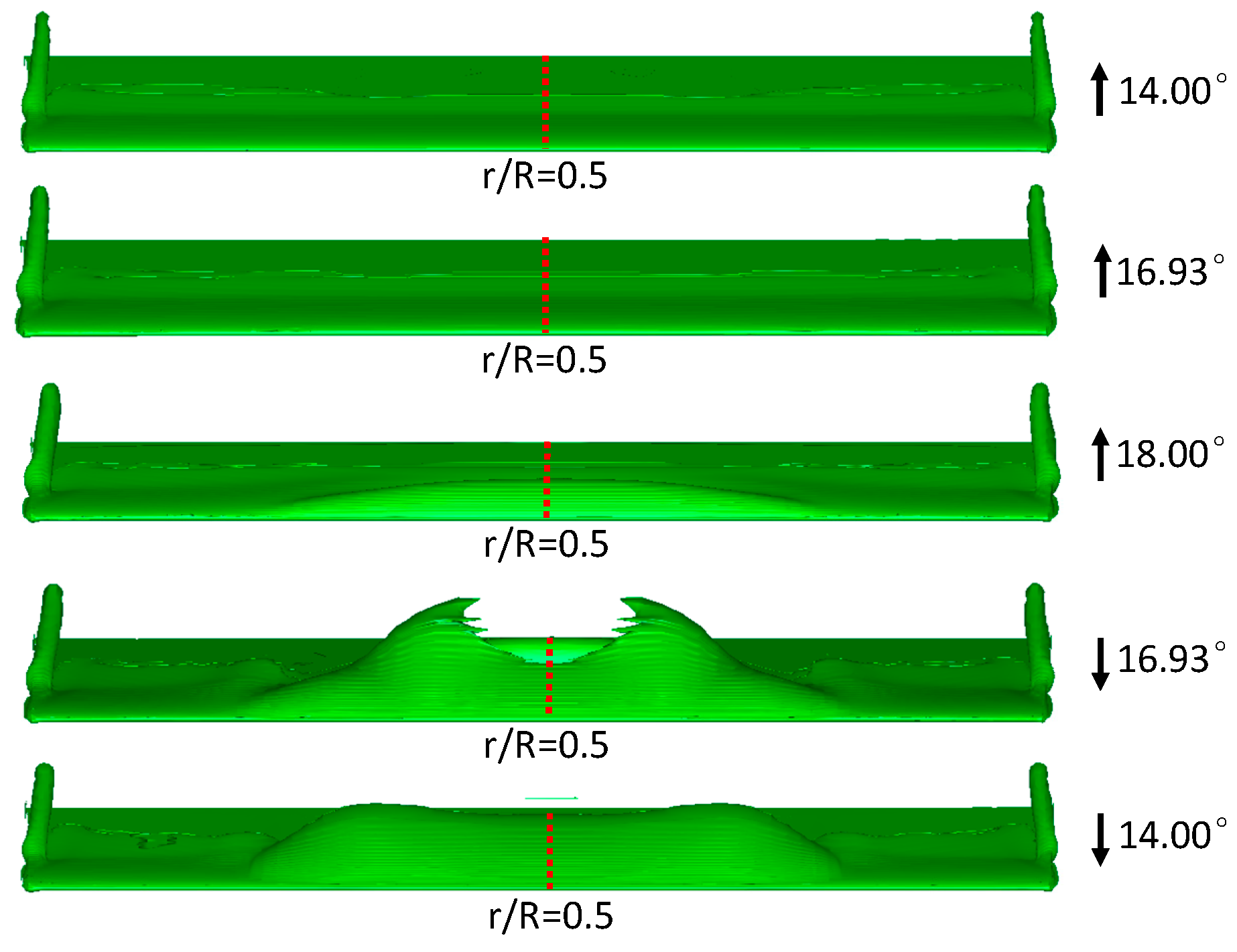
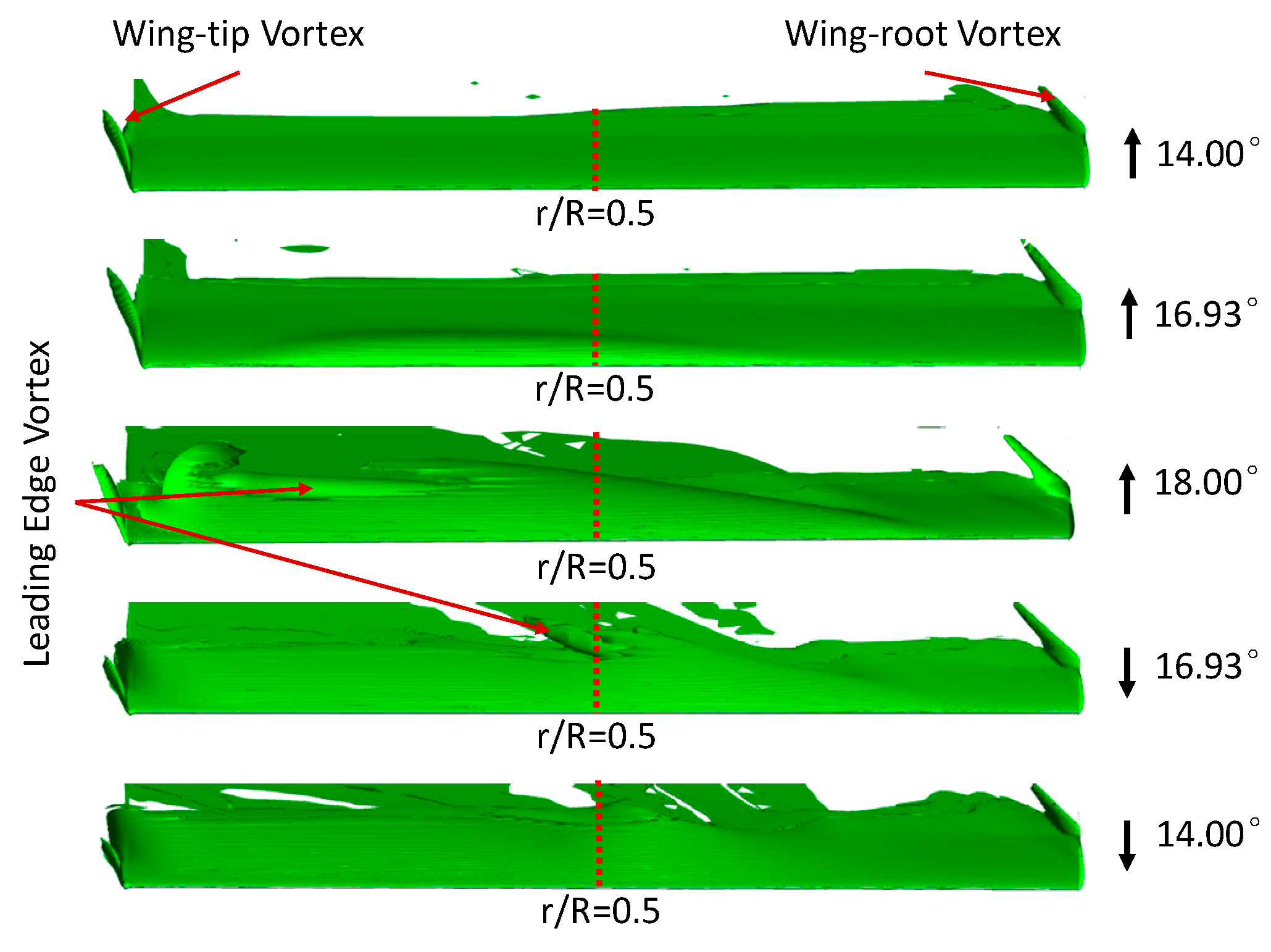
Aiming at investigating the interaction between the dynamic-stall and wing-tip vortices, the dynamic-stall characteristics of the finite wing were simulated at Ma = 0.3, k = 0.075, and $\alpha ={10.0}^{\circ }-{8.0}^{\circ }\sin (\omega t)$. Equal-vorticity (8.0) surfaces, normalized by ${\rho }_{\infty }{V}_{\infty }^2$ at different AoAs, are shown in Figure 4. It is illustrated that vorticity distribution is basically symmetric, and wing-tip vortex variation at different AoAs is not obvious. With the increase of AoA (↑), the dynamic-stall vortex first forms near the leading edge of the finite wing at r/R = 0.5. 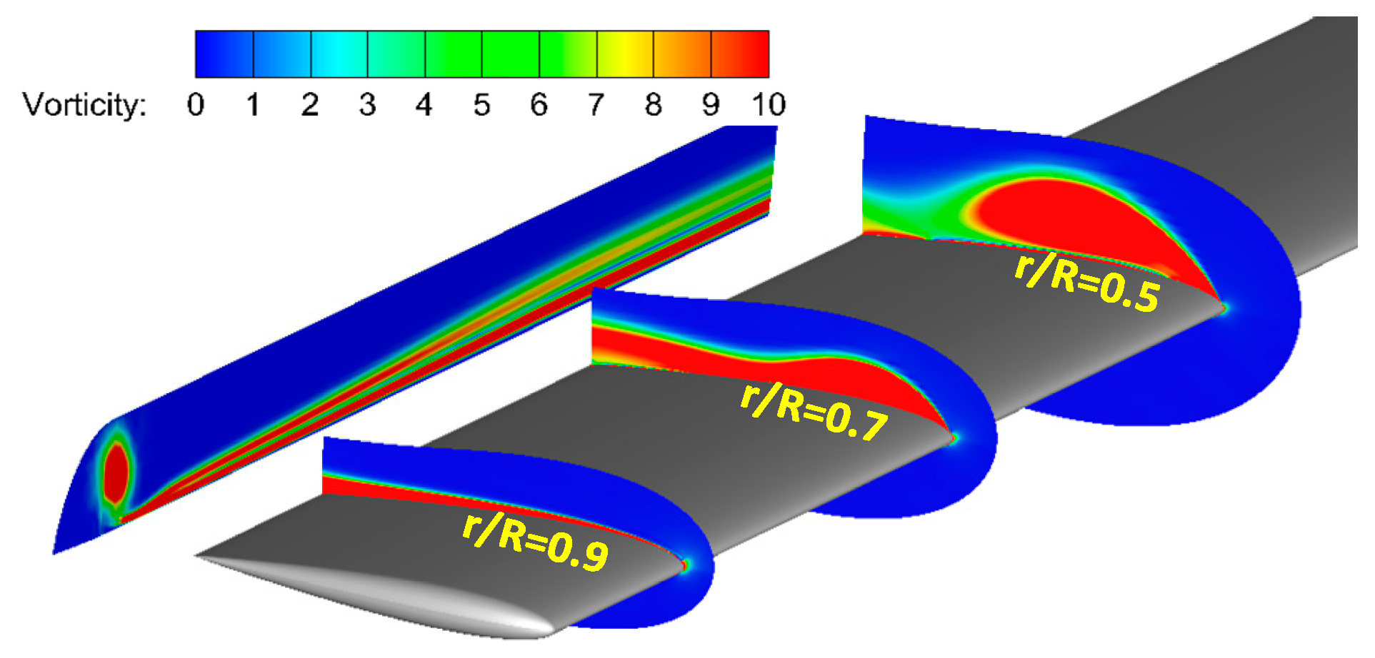At an AoA of 16.93° in the downstroke process (↓), it is illustrated that the dynamic-stall vortex separates from the upper surface of the wing at r/R = 0.5, and reattaches itself on the wing surface when it extends to the wing tip and wing root. The vorticity of the leading-edge vortex (LEV) with $\alpha ={16.93}^{\circ }$ (↓) at different wing sections (r/R = 0.5, 0.7, 0.9) is shown in Figure 5. It is also illustrated that maximum LEV vorticity is at r/R = 0.5, and vorticity decreases when the blade sections get close to the wing tip.

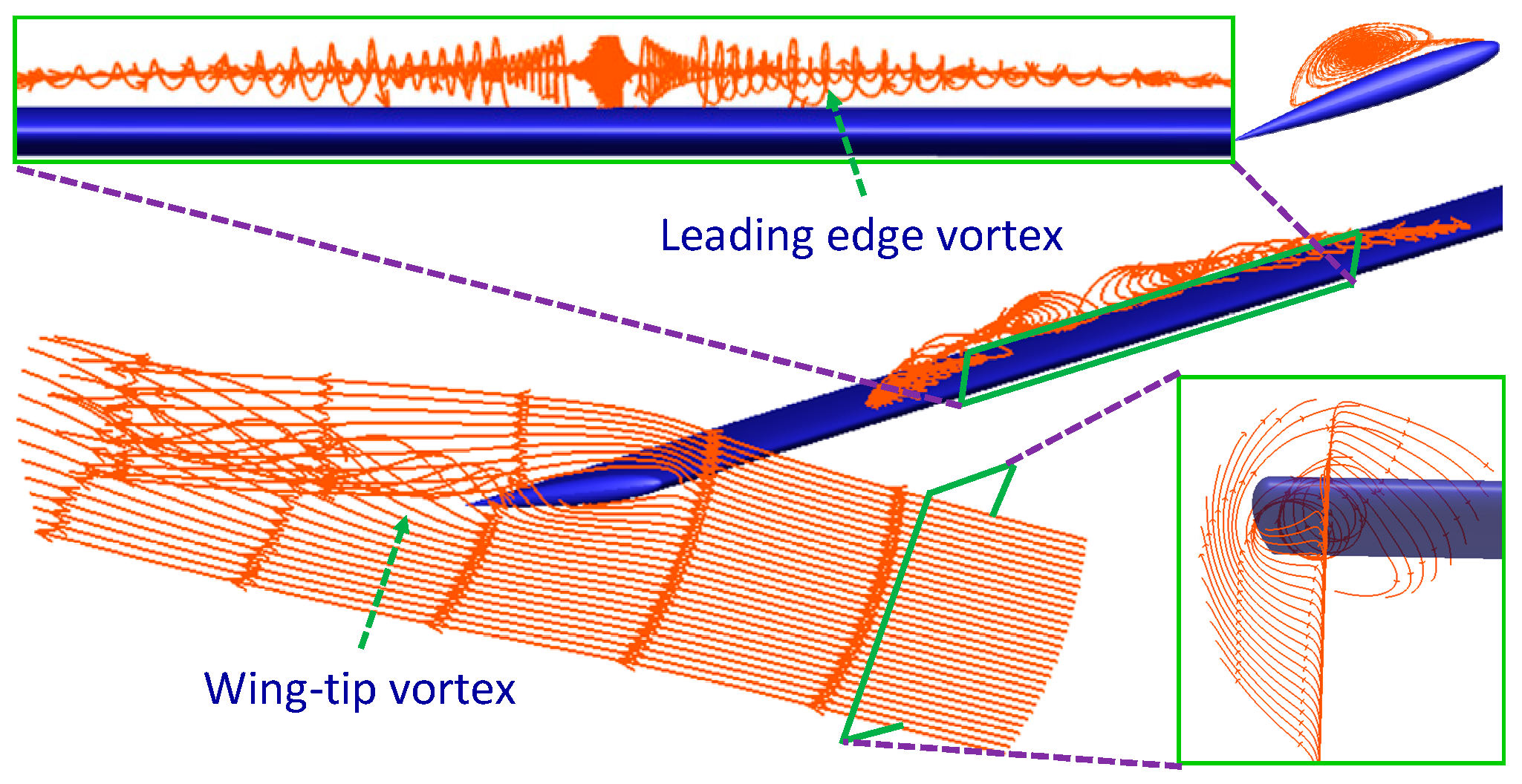
In order to display the vortex structure, the spatial streamlines of the finite wing are shown in Figure 6. It is illustrated that the LEV is symmetrically attached to the upper surface. In addition, airflow is rolled up from the lower surface near the wing tip due to the pressure difference of the wing surface, and then the clockwise wing-tip vortex forms on the upper surface and convects to the wing wake.

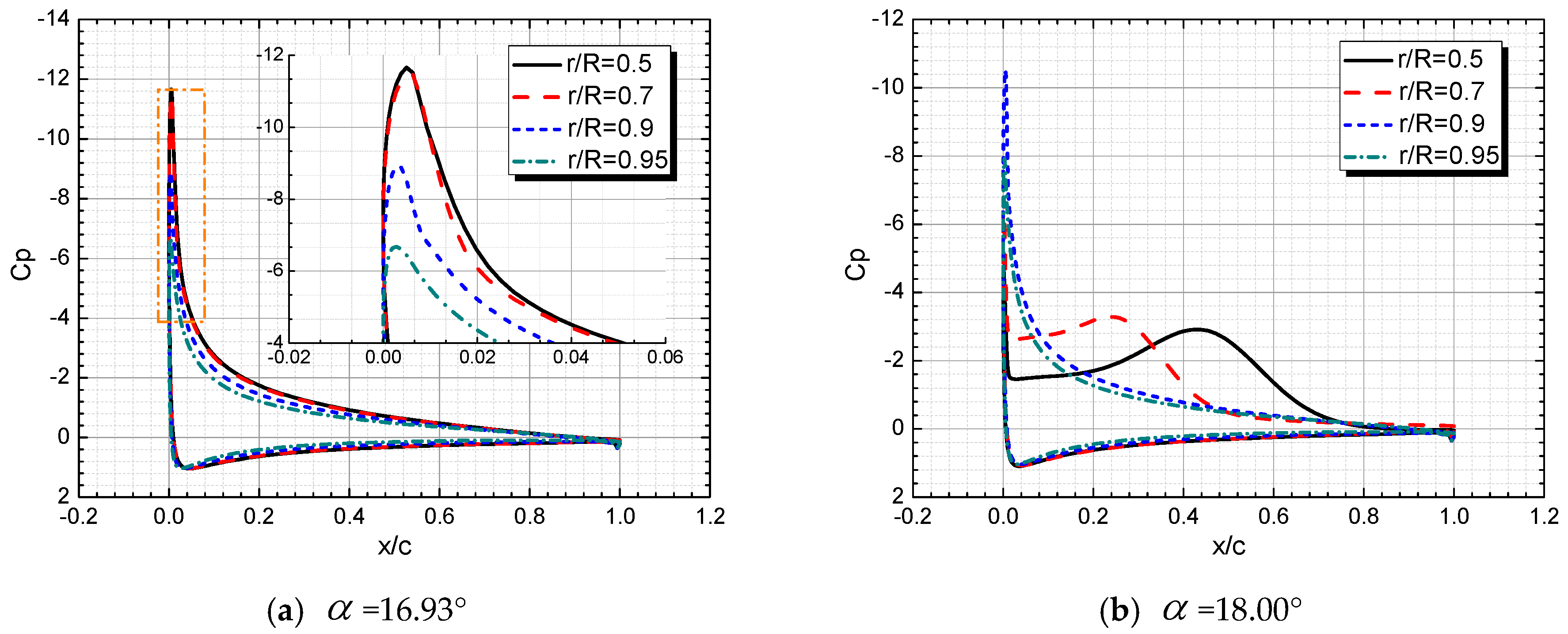
Aiming at illustrating the variations of aerodynamic loads induced by the wing-tip vortex, pressure coefficient (Cp) wing distribution at an AoA of 16.93° and 18.00° is respectively shown in Figure 7. It can be seen from Figure 7a that Cp peaks would decrease when the wing section gets close to the wing tip due to the effect of the wing-tip vortex. As a result, the adverse pressure gradient is also decreased. It is illustrated in Figure 7b that Cp distribution on the upper surface is obviously influenced by LEV at r/R = 0.5 and 0.7. However, the LEV effect on Cp distribution is not obvious near the wing tip. It is indicated that the wing-tip vortex could effectively restrict the LEV.

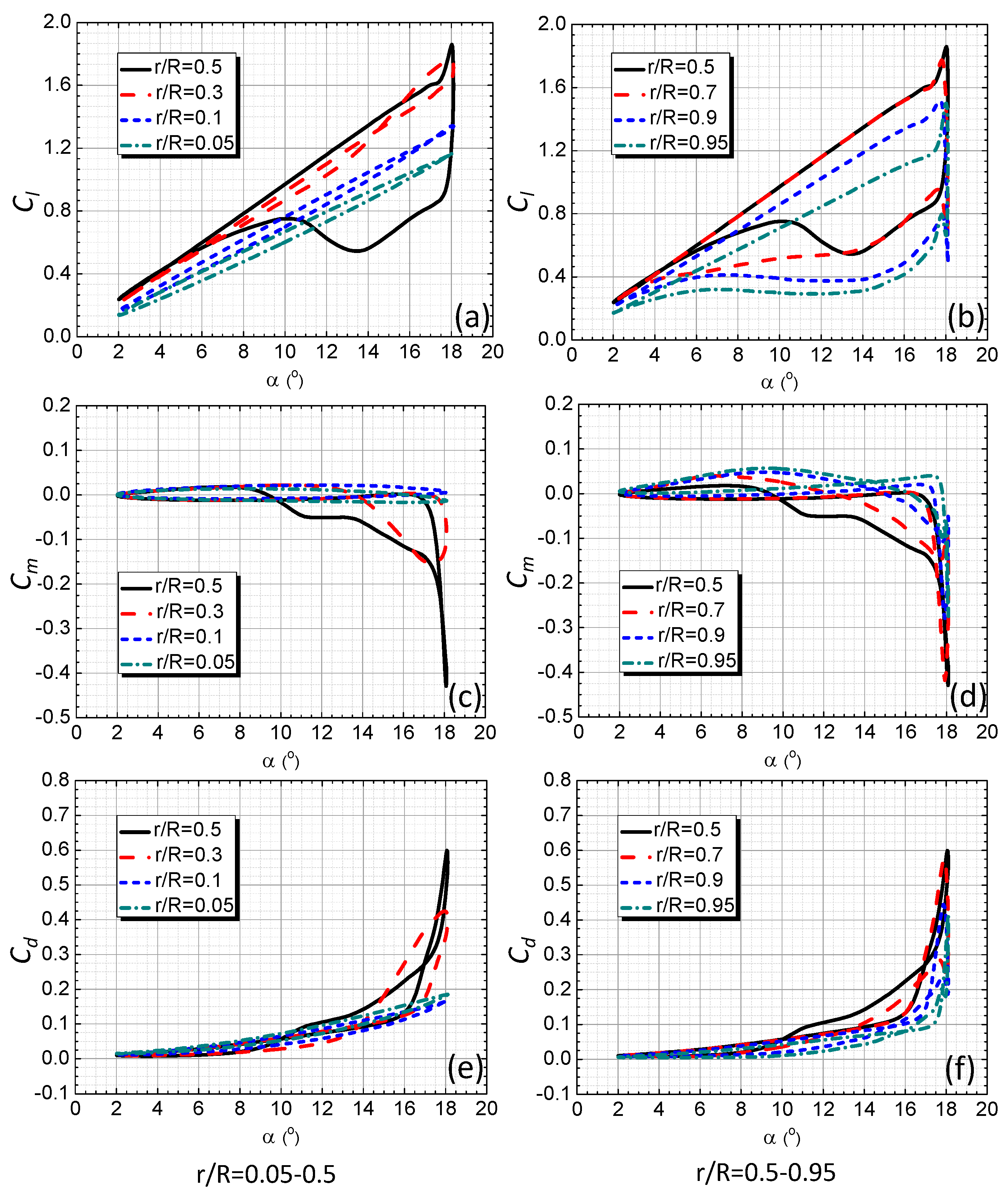
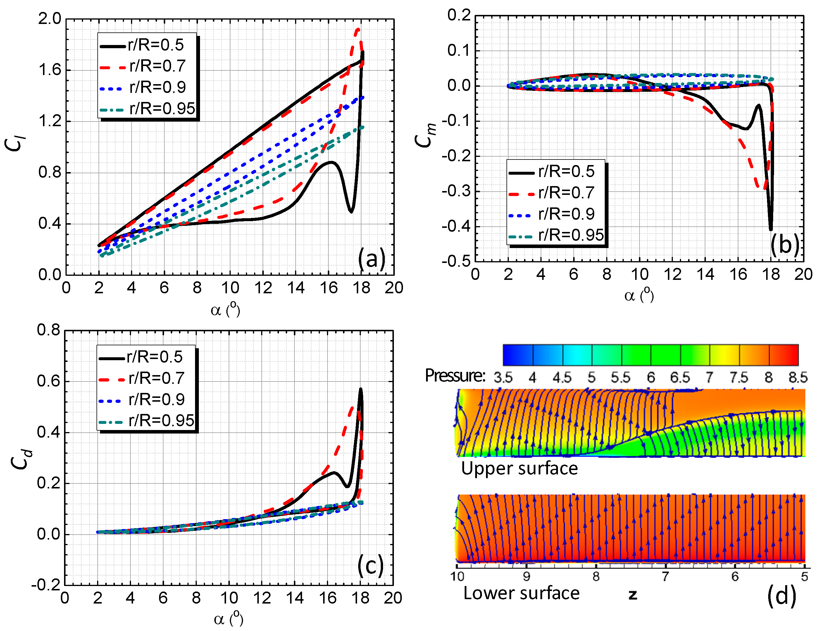
The comparison of dynamic-stall load at different wing sections (r/R = 0.5, 0.7, 0.9, and 0.95) are shown in Figure 8. It is illustrated that the lift curve slopes of C_l decrease in the upstroke process, and lift-stall characteristics are alleviated when the wing sections get close to the wing tip. This is maybe due to the pressure difference between the upper and lower wing surface being decreased by the unloading effect of the wing-tip vortex. As a result, the peaks of pitching moment coefficient C_m and drag coefficient C_d are also decreased. Pressure (normalized by ${\rho }_{\infty }{V}_{\infty }^2$) and streamline distributions at $\alpha ={18.00}^{\circ }$ are also shown in Figure 8 (only half the wing is shown due to flowfield symmetry). It is illustrated that airflow is separated from the upper surface at a span of r/R = 0.5–0.8 due to the effect of LEV. As a result, pressure on the upper surface is obviously reduced, and the lift would keep increasing with the AoA until the vortex is shed from the wing surface.

3.2. Finite-Wing Dynamic Stall with Spanwise Flow

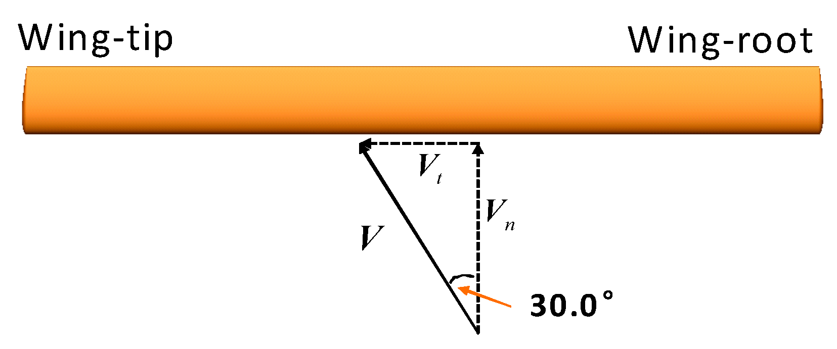
Due to the forward-flight effect, spanwise flow appears on the rotor blade, and spanwise-flow velocity changes with different rotor azimuths. As a result, spanwise flow is a critical-influence factors on the unsteady aerodynamic characteristics of a rotor. Therefore, in order to research the effects of the spanwise flow on the dynamic stall, an inflow angle of 30.0° (deviated from the vertical direction) is considered in this study, as shown in Figure 9, where V, V_n, and V_t represent the resultant velocity, normal velocity, and tangential velocity, respectively. In this case, AoA variation was $\alpha ={10.0}^{\circ }-{8.0}^{\circ }\sin (\omega t)$, the Mach number of $V_n$ was 0.3, and reduced frequency was 0.075 (normalized by $V_n$).

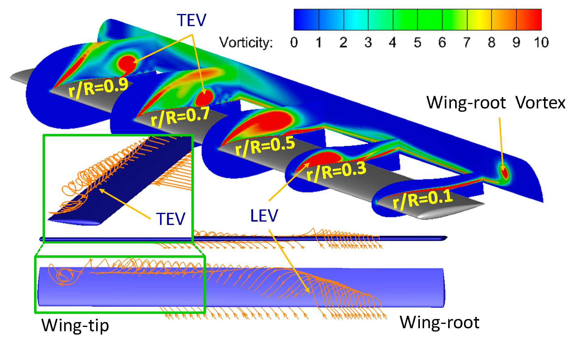
Figure 10 shows equal vorticity surfaces (vorticity is 7.5) of the wing at different AoAs. It is illustrated that vortex structures of a finite wing with a spanwise flow are very different from the vortex structures with a nonspanwise flow. First, the wing-tip and wing-root vortices have an inclination angle of 30.0° along the freestream. Second, the LEV is accumulated near the wing tip and is restricted near the wing root due to the influence of the spanwise flow. In addition, the LEV bursts and sheds from the upper surface near the middle part of the wing due to nonuniform vorticity accumulation. The vorticity contours of the dynamic-stall vortex at different wing sections are shown in Figure 11. It is clearly illustrated that the LEV and trailing-edge vortex (TEV) near the wing tip (r/R = 0.9) shed earlier compared with those near the wing root (r/R = 0.1). It is indicated that the spanwise flow of the finite wing could promote dynamic stall near the wing tip, and delay it near the wing root.

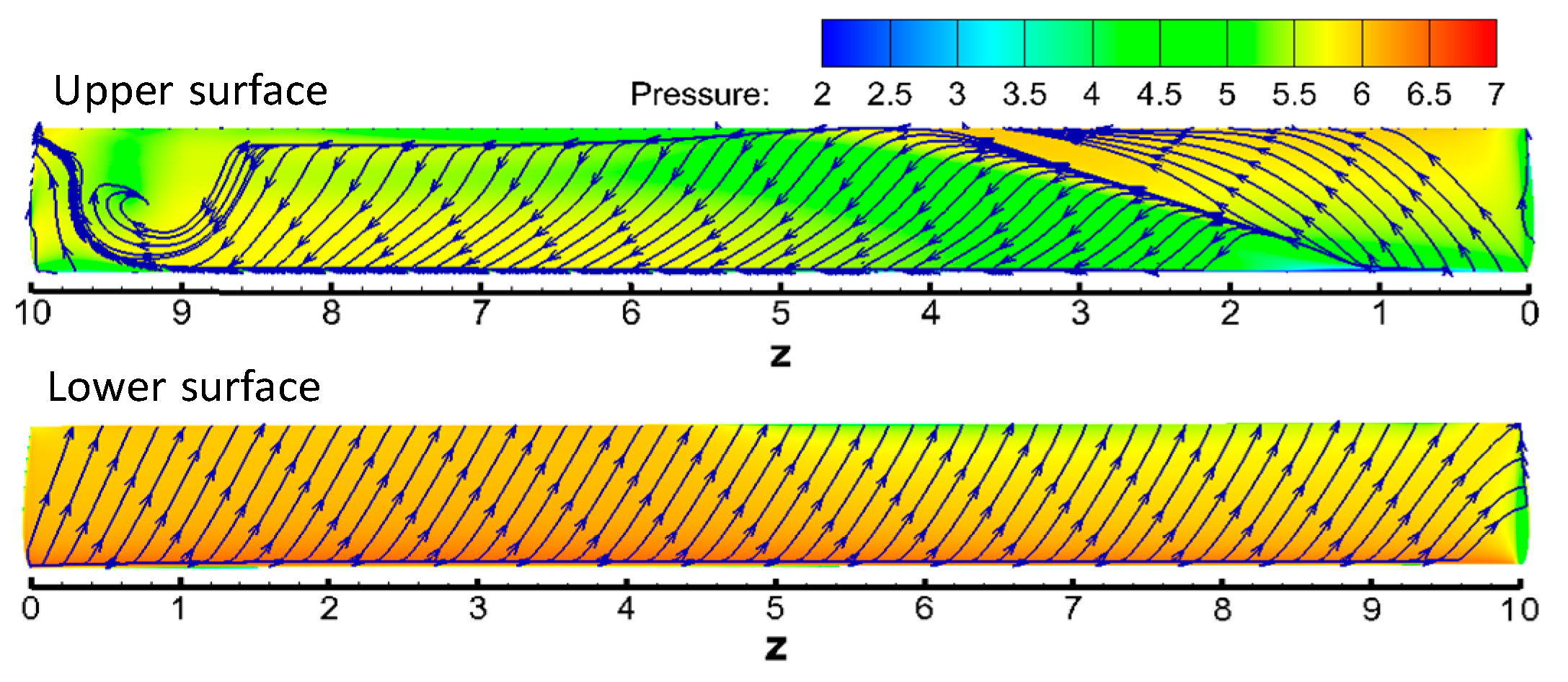
The pressure and streamline distributions of the finite wing on the upper and lower surfaces at $\alpha ={18.00}^{\circ }$ are shown in Figure 12. It can be seen that airflow convection near the wing surface is contrary to the freestream flow due to the influence of LEV. As a result, airflow separation appears on the upper surface. In addition, it can be seen from the streamlines on the upper surface that an irregular flow appears near the wing tip (r/R = 0.9–1.0) due to the interaction of the wing-tip vortex with the spanwise flow. On the contrary, streamlines on the lower surface are more stable compared with the upper surface, and streamlines on the lower surface regularly incline to the wing tip due to the effect of the spanwise flow. It can also be seen that streamline inclination angles are increased when they get close to the wing tip due to wing-tip vortex induction.

Comparisons of C_l at different wing sections are shown in Figure 13. It can be seen from the C_l curves that C_l presents light dynamic-stall characteristics near the wing root. Meanwhile, the slopes of the lift curves were also decreased due to the effect of the wing-tip vortex. On the contrary, the unsteady characteristics near the wing tip present deep dynamic-stall characteristics. It can be seen that the slopes of the lift curves were also decreased. However, the decrement is smaller than that of the wing root (symmetrical sections). This is maybe due to LEV induction being more obvious for the wing tip since LEV is stronger. From the comparison of C_m curves at different wing sections in Figure 13, it is illustrated that C_m peaks are decreased when the sections get close to both the wing tip and wing root. However, the C_m peak at the wing root is smaller than that of the wing tip, because the dynamic-stall vortex is restricted by the spanwise flow. As a result, C_m variations near the wing root are much gentler than those of the wing tip. From the comparison of C_d curves at different wing sections in Figure 13, it is illustrated that C_d peaks near the wing root are smaller than those of the wing tip due to the restriction of LEV. As a result, it is indicated that the vorticity collection induced by the spanwise flow could significantly affect the dynamic-stall characteristics of a finite wing.

3.3. Rotor-Blade Dynamic Stall

Helicopter rotors usually have the dynamic-stall phenomenon appear in the retreating side in forward flight due to the cyclic pitch movement of the rotor blade. In order to research rotational influence on dynamic-stall characteristics, a simplified case was performed based on finite-wing research. The used rotor in this study had two rectangular blades, and the shape of the rotor blade was the same as the finite wing. In this case, numerical simulation was performed at an advance ratio of 0.3 with blade-tip Mach number of 0.6. To dismiss the interaction of the subordinate influence factor on rotor dynamic stall, the cyclic pitch of the rotor blade was simplified as $\alpha ={10.0}^{\circ }-{8.0}^{\circ }\sin (\omega t)$.

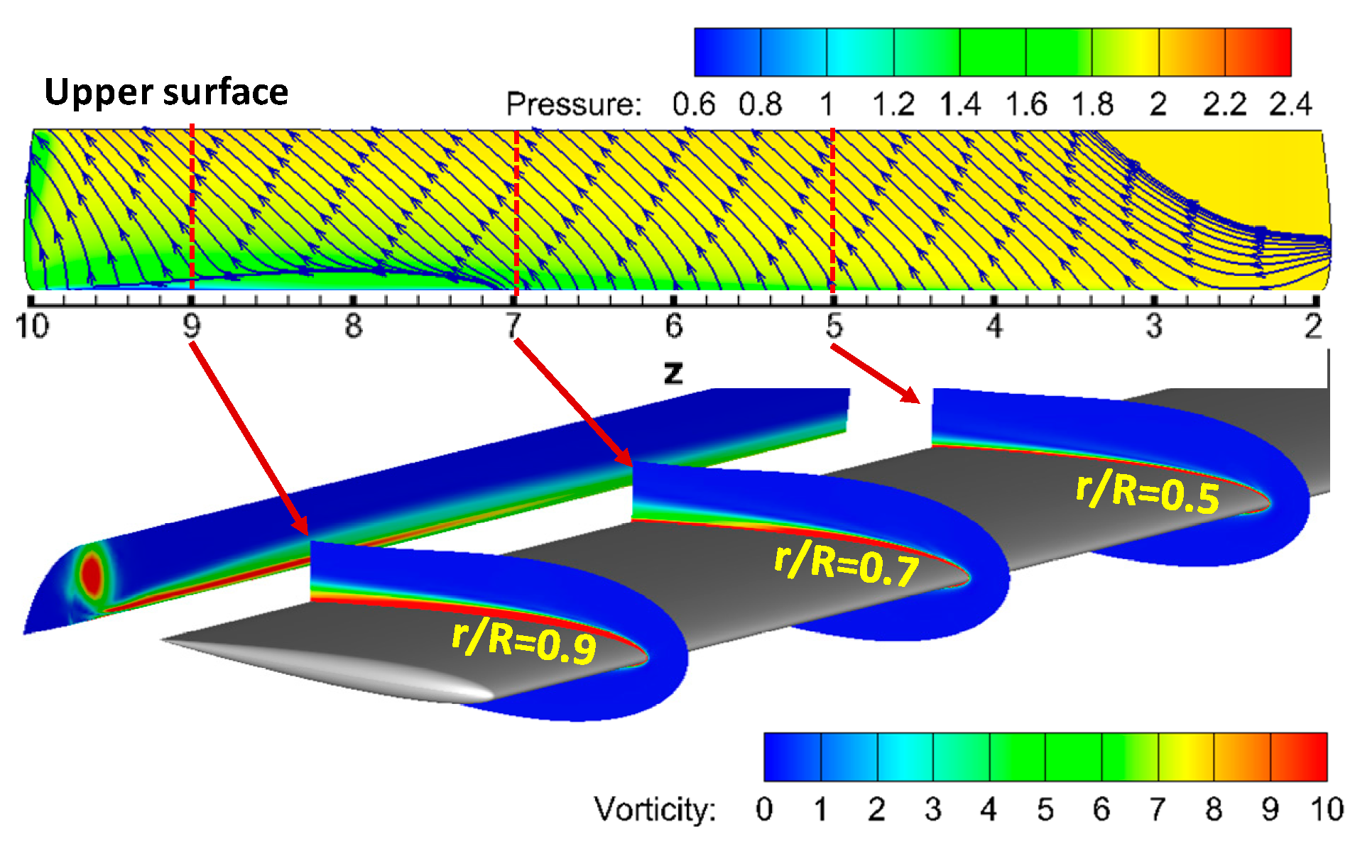
Streamline and vorticity contour distributions at $\alpha ={18.00}^{\circ }$ on the surface of the rotor blade at an azimuth of 270° are shown in Figure 14. It can be seen that a small airflow-separation region appeared on the upper surface from r/R = 0.7 to 0.9. It can also be seen that streamlines inclined to the blade tip. This may be attributed to the rotational motion of the blade, because airflow near the blade surface would follow with blade rotation due to airflow stickiness. Therefore, airflow convects to the blade tip due to centrifugal force. From the vorticity contours of the dynamic-stall vortex at different blades, it can be seen that vorticity basically concentrates on the blade surface. This means that no obvious LEV forms and sheds under this condition, which is very different from the finite-wing case. As a result, it is indicated that the dynamic stall of the rotor blade would be restricted.

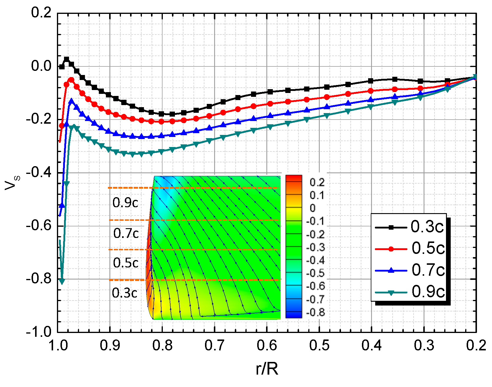
In order to analyze spanwise velocity characteristics, spanwise velocities (normalized by blade-tip velocity) at different chord positions are shown in Figure 15 ($\alpha ={18.00}^{\circ }$), and these data were calculated at a normal distance of 0.001 c from the blade surface, where c represents the chord length of the blade. It can be seen that spanwise velocity is basically enlarged with the increase of blade radius. This variation can be attributed to centrifugal force being larger when radius increases. As a result, airflow would more obviously be accelerated, and spanwise velocity would be larger. Moreover, it could be seen that spanwise velocity is also enlarged with the increase of chord position at the same blade radius. This is due to airflow acceleration time along the blade surface increasing as chord position gets close to the trailing edge of the blade. Another characteristic that should be noticed is spanwise velocities decreasing near the blade tip because the induced velocity of the blade-tip vortex points to the blade root on the upper surface.

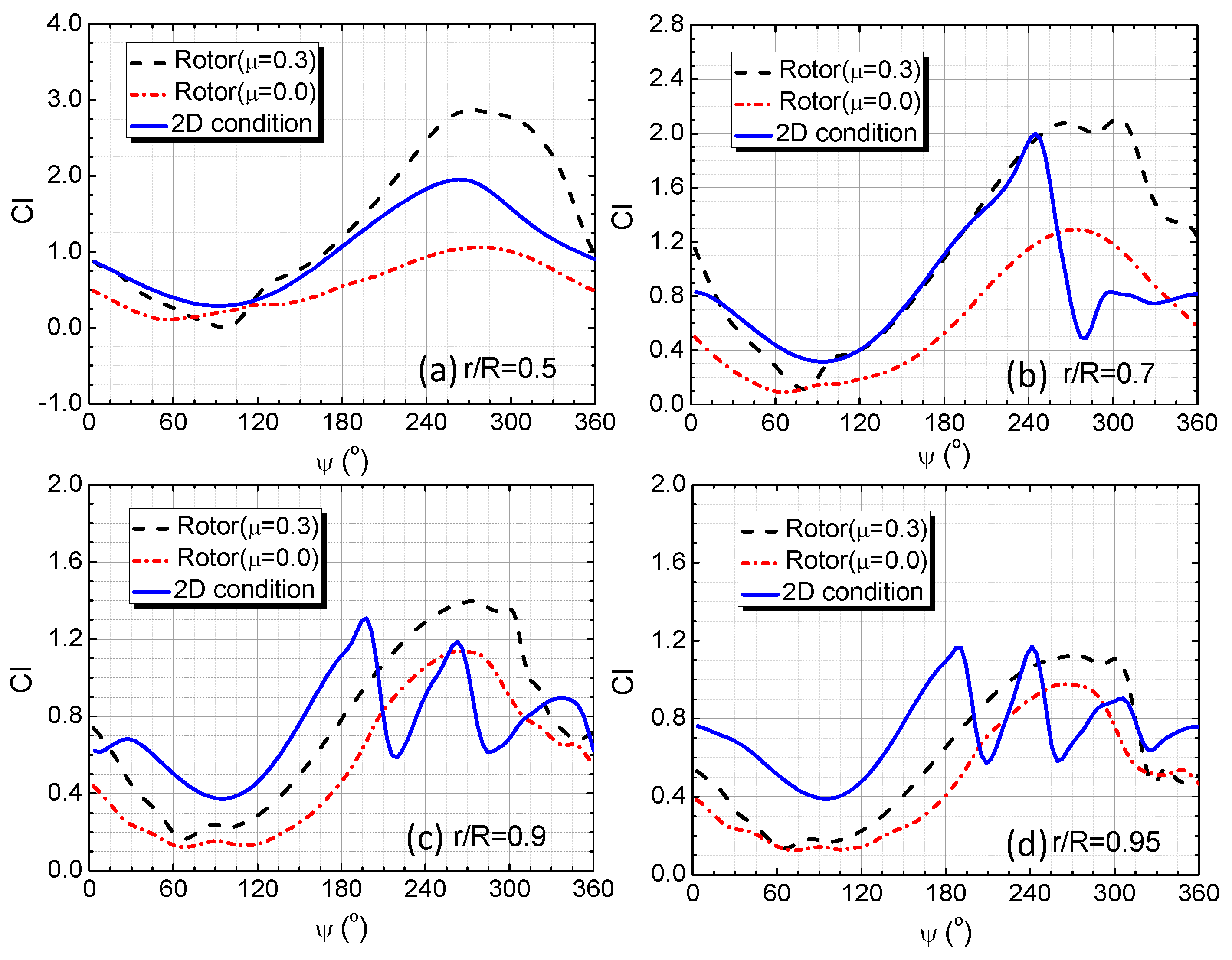
The comparison of C_l curves between the different blade sections and the 2D airfoil is shown in Figure 16. The dynamic-stall characteristics under a 2D condition are simulated under variational freestream velocity, i.e., $Ma=0.6\cdot \lambda -0.18\cdot \sin (\omega t)$, where $\lambda$ represents blade section. AoA variations are the same as those of the rotor blade, i.e., $\alpha ={10.0}^{\circ }-{8.0}^{\circ }\sin (\omega t)$. By comparing the simulated rotor results with $\mu =0.0$ and $\mu =0.3$, it can be seen that rotor C_l with $\mu =0.3$ is larger than that of $\mu =0.0$ at different blade sections, because downwash airflow in forward flight is smaller than that in hovering flight. As a result, effective AoA decrement is smaller in forward flight. It can also be seen in the figure that the deviation between the two rotor conditions is decreased with the increase of the blade radius, because downwash airflow would be reduced near the blade tip.

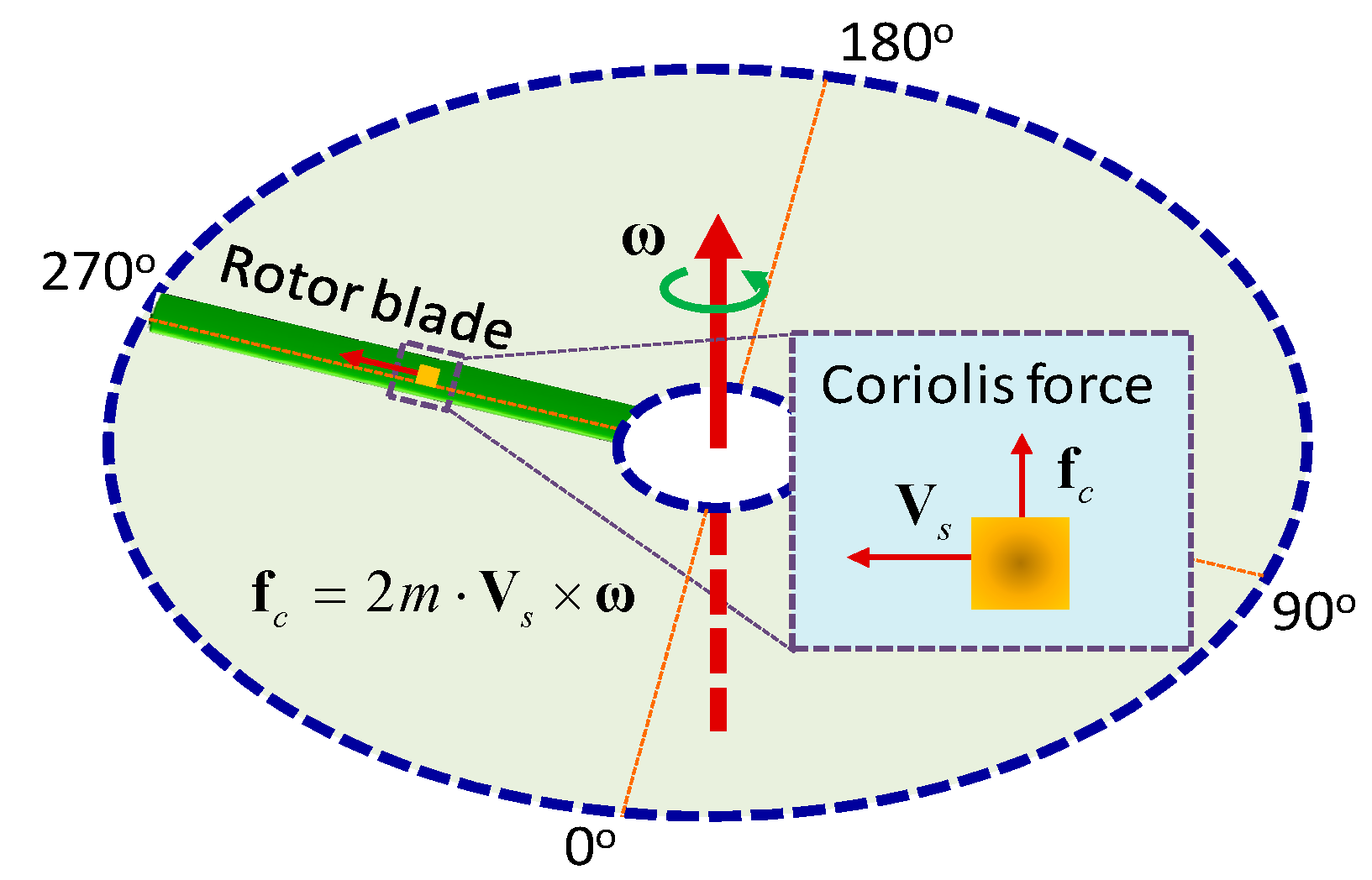
Another observation is that dynamic stall occurs on the 2D airfoil. However, dynamic stall is not obviously on the rotor blade. One of the reasons is that airflow in the boundary layer of the blade surface would receive additional force due to Coriolis force, as shown in Figure 17. It can be seen that airflow would get velocity pointed to the trailing edge of the blade. As a result, airflow separation would be restricted, and the LEV would be alleviated.

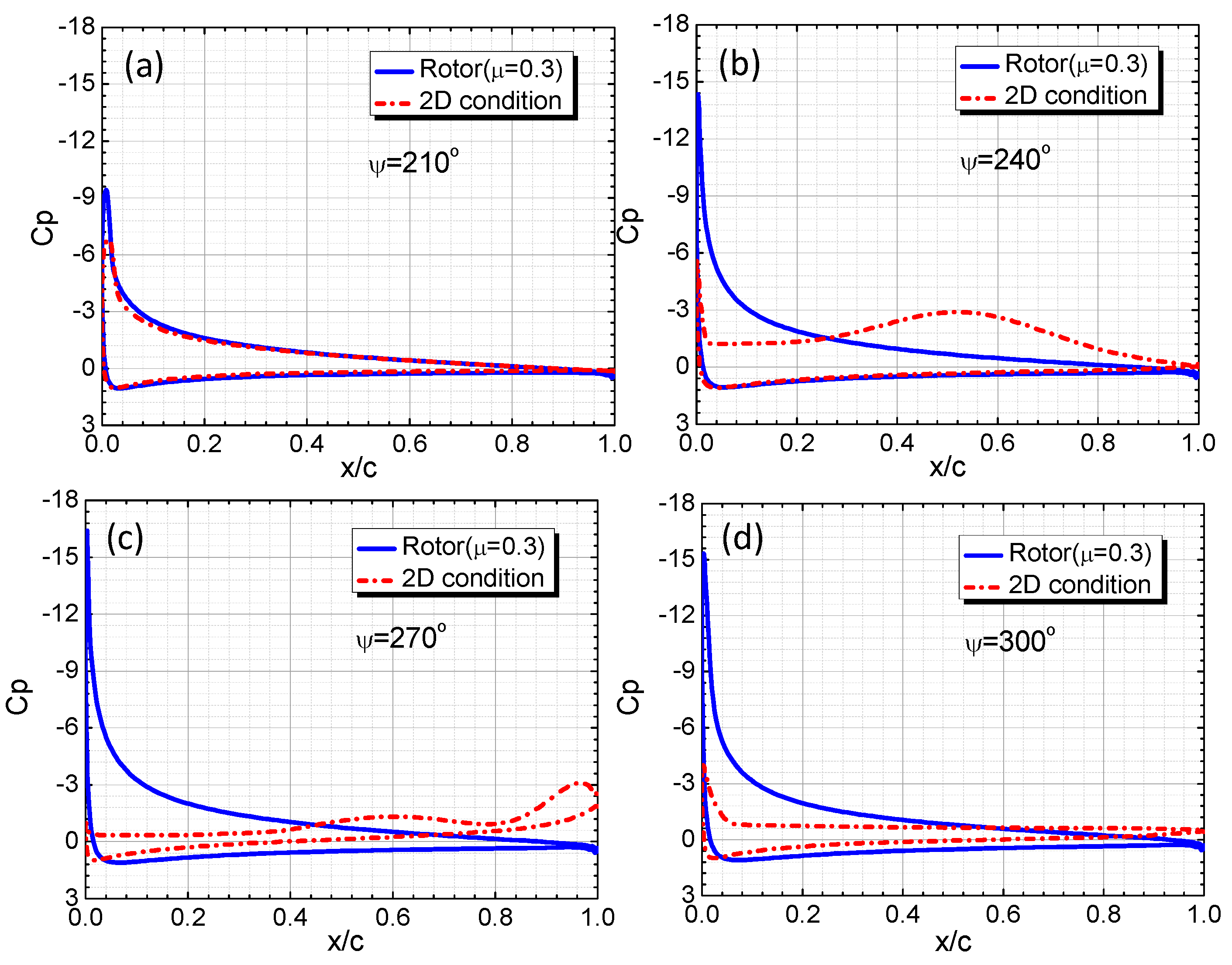
In order to analyze the rotational influence of a rotor blade on dynamic-stall characteristics, Cp distribution at r/R = 0.7 is shown in Figure 18. It is indicated in Cp distribution that the adverse pressure gradient of a 2D airfoil is larger than that of the rotor. As a result, airflow separation occurs on the upper surface of the airfoil, and LEV transport occurs from the leading edge to the trailing edge, as shown in $\psi ={240}^{\circ }$ and $\psi ={270}^{\circ }$.

4. Conclusions

In this study, the unsteady CFD method was employed to simulate the dynamic-stall characteristics of a finite wing and rotor. Results can be summarized as:

(1) The LEV of the finite wing would be restricted near the wing tip and wing root due to the influence of the wing-tip vortex. As a result, the dynamic stall of the finite wing is alleviated near the wing tip and wing root.

(2) Spanwise flow would cause LEV accumulation along the wing. Therefore, the dynamic stall of the finite wing is alleviated near the wing root and aggravated near the wing tip.

(3) For the rotor blade, boundary-layer separation is delayed by the effect of the Coriolis force and spanwise flow. As a result, dynamic-stall characteristics are restricted. This result could be used to guide rotor-airfoil shape design in the future research.