An Artificial Bee Colony Algorithm Based on a Multi-Objective Framework for Supplier Integration

Featured Application

Supplier chain management, Industry production, Efficient industry management, global business management, smart manufacturing.

Abstract

Modern day industries strive to obtain long-term supplier integrations (SI) with potentially stronger supplier groups, to achieve fast and reliable production. This paper studies the process of selecting vendors, while simultaneously considering the aspects of random factors, multiple criteria, and efficiently reaching optimal solutions to improve the SI. A framework was developed that consists of three layers of expert opinions, supplier requirements, and multi-objective bee colony optimization. The model factors affecting the SI decision were explored from the comprehensive relevant literature, and these factors were shortlisted and prioritized. Routines for the modeled framework were coded by using the proposed algorithms which were implemented for a real-world problem from a manufacturing small and medium enterprise (SME) in Pakistan. Optimization of SI was carried out on an archived artificial bee colony (AABC). Its effectiveness was also evaluated by comparison with simple artificial bee colony (ABC) and particle swarm algorithms. The methodologically calculated results, obtained from simulation of a mathematically reinforced optimization framework, are highly beneficial for the industry, as well as local and international suppliers. A detailed and in-depth evaluation of suppliers was provided by the sensitivity analysis, which presented a more rigorous authentication and elaboration of the results. The presented framework is the first of its kind for the SMEs of Pakistan and can be applied with little modification to other industries.

1. Introduction

In the prevailing swiftly changing global business environment, process and manufacturing industries are facing different challenges regarding product reliabilities, production costs, on-time availabilities of raw material, procurement times, etc. About 70% of the average product cost is incurred in the purchase of raw materials [1]. If companies fail to develop competitive products due to higher raw material costs, they may face serious issues regarding customer satisfaction and financial stability. The timely availability of raw materials is an additional major challenge. In the current competitive business climate, companies cannot afford undue delays in supply orders. From small industries to mega projects, the supply chain plays an important role in achieving production goals [2].

A sound number of these challenges can be successfully handled if enterprises can develop long-term win-win relationships with well-matched international and national prospective suppliers. Therefore, the concept of supplier integration (SI) has been recently proposed by different researchers to enable enterprises to conveniently cope with these dynamic supply chain business issues [3,4,5,6]. SI is the concept for improving the part of the supply chain between manufacturers and their respective suppliers of ingredients, raw materials, packaging, etc. By sharing information between parties, the suppliers and buyers are able to exercise judgment on costs, quantities, timing of deliveries, production streamline product flow, and to create a collaborative relationship [7]. However, this strategy is coupled with a number of problems. The demographic location of countries, their economic status, product categories, and the capabilities of suppliers are some of the main factors affecting the decision regarding selection of suppliers and long-term integration with the manufacturer [8].

The literature shows that different factors were used in previous research by different authors in the field of SI. Some of these factors are market pressure, government interference, firm size, technology [9], production costs, long-term relationships, information sharing, reliability, quality, flexibility [10,11,12,13], lead time, financial status, technical capability, and after-sale support [14,15,16]. Studies have been reported by various authors on: SI in sales and operations in the Asia-Pacific region [17], SI in strategic sourcing and supplier evaluation accommodating critical success factors in the UK and Germany region [18], and a study of multiple-criteria supplier selection in fuzzy environment based in agri-food industry in Australia [19]. A case of grey-fuzzy multi-objective model for a supplier selection in Pakistan, discussed by [20] is based on the planning of production and distribution to ensure product’s safety. However, development of framework for SI and supplier selection for SME’s through a meta-heuristic application in such countries is rarely seen in literature.

In view of the above mechanisms, this paper proposes a framework which is composed of an archived artificial bee colony algorithm, based on multi-objective optimization. The factors affecting these supplier selection decisions were screened from the relevant literature under the guidance of industry experts to ensure suitability with respect to the current environment of the selected country. The systematically composed framework, which was founded on multi-objective optimization, was uniquely applied to a real-world SI problem of an actual SME.

In Section 2, methodologies used for SI and background of the artificial bee colony (ABC) are reviewed. In Section 3 the developed framework is discussed. Data specific solutions are explained in Section 4, while results and conclusions are discussed in Section 5 and Section 6 respectively.

2. Methodologies Used

Depending upon the criteria of influence and nature of the SI problems, different multi-criteria decision-making techniques and other optimization and analytical techniques were used by different authors for the evaluation of suppliers. Multi-criteria techniques are widely used in decision making [21]. Some of the most recently used methodologies are mentioned here as examples. A correlation and regression analysis for supplier development has been implemented for a four-phase analytic hierarchy process with quality function deployment (AHP-QDF) based multiple-criteria decision analysis (MCDM) approach [22,23]. The authors in [15] applied a supplier development program with a gray-AHP algorithm. A model for supplier development using the partial least square structural equation model (PLS SEM) was developed in [24]. The authors in [25] recommended that the selection of suppliers for SI be done through some non-traditional multi-objective optimizations. A Bayesian information criteria (BIC) approach was evaluated in [26].

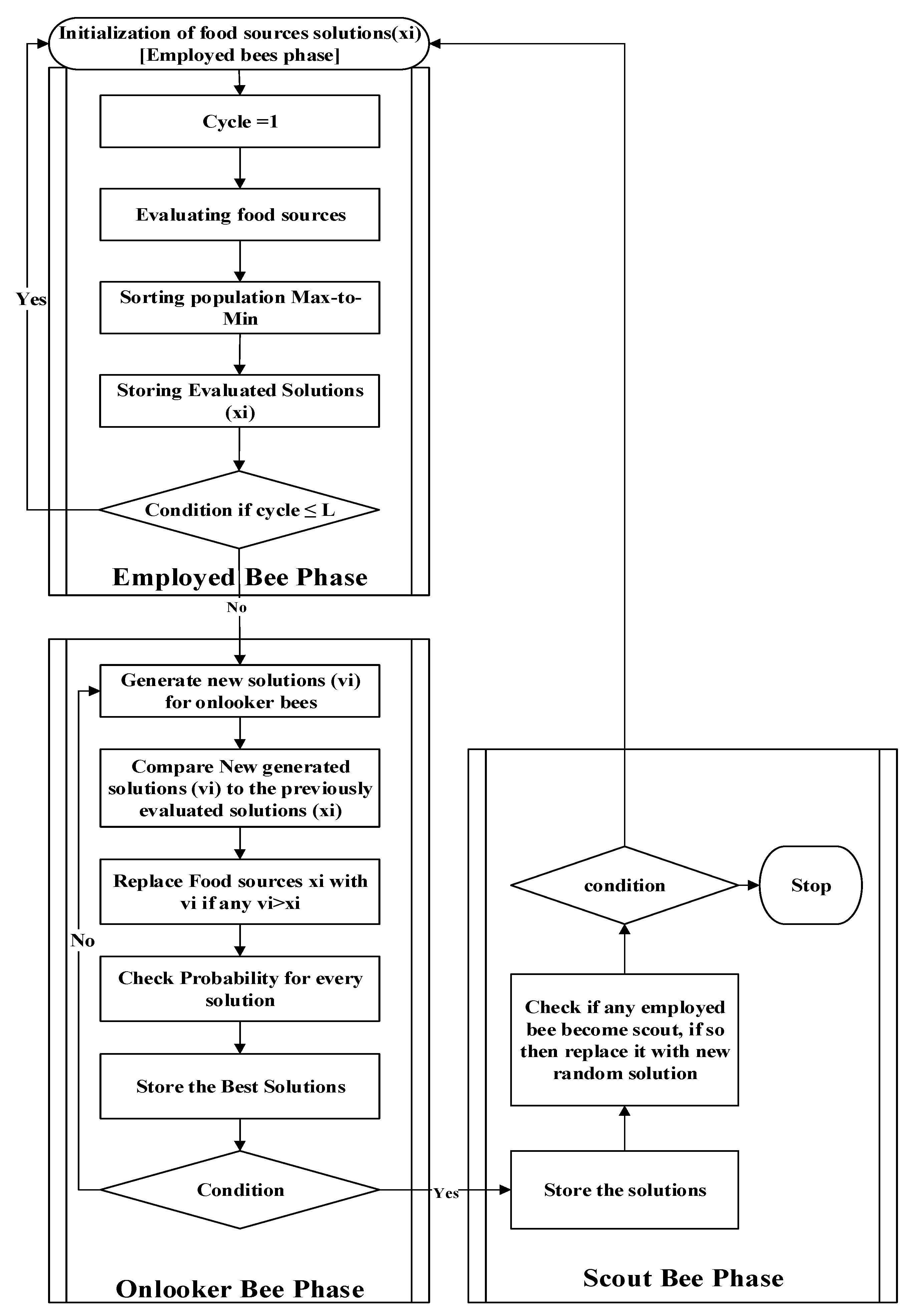
3. Background of ABC

In the present research, a modified artificial bee colony (ABC) algorithm, i.e., the archived ABC (AABC) is used to evaluate the developed framework for SI. The ABC technique is one of the latest and fastest processing algorithms for solving multi-objective problems. In [27], the ABC algorithm was introduced for the first time. It simulates the foraging swarm behavior of honey bees uses very few control parameters, and shows fast and efficient results. The researchers in [28] demonstrated that, for multimodal or multivariable problems, the ABC approach produces better results than other algorithms. Reasons for using the ABC algorithm in this study include its swift processing and optimized results. A number of the studies that offered a comparison of ABC with other multi-objective algorithms are compiled in

Table 1. Artificial bee colony (ABC) Comparison in the Literature.

ABC Comparison
Reference	Comparison of Algorithms	Selected Algorithm	Application
Özbakir [51]	Bees Algorithm (BA), Genetic Algorithm (GA)	BA	Continuous Optimization
Fahmy [22]	Particle Swarm Optimization (PSO), BA	BA	Speed parameters for wind turbine generators
Yuce [53]	Swarm Optimization Algorithms (SOAs), Bee Colonial Optimization (BCO), GA, ABC	ABC	Honey bees-inspired optimization method
Delgado-Osuna [54]	GA, state-of-the-art algorithm, ABC	ABC	Problem of composing medical crews
Karaboga [28]	Differential Evolution (DE), GA, PSO, ABC, Evolution Strategy (ES)	ABC	Comparative study of Bees Algorithm
Pham [55]	GA, K-means, BA	BA	Data clustering
Karaboga [28]	ABC, PSO	ABC	Clustering Approach
Bouaziz [57]	ABC, PSO,	ABC	Iris Image optimization
Karaboga [56]	ABC, PSO.	ABC	Multi Objective Optimization

to further justify its use.

The rapid development of technology and economy has increased the consumption and waste of electronic products. Recycling and recycling valuable and hazardous parts of used electronic products can effectively save resources while reducing environmental pollution and promote coordinated development of economy and environment. As one of the most critical aspects of the recycling process, its efficiency directly affects the cost of remanufacturing [29], thus, the disassembly line balance problem (DLBP) has gradually received attention. Gupta et al. [30] proposed DLBP, and the establishment of a simple mathematical model for the DLBP. Subsequently, precise mathematical methods and meta-heuristic algorithms were mainly used to optimize DLBP literature. The authors in [31,32,33,34] proposed a method using traditional mathematical programming based on different strategies. The method solves DLBP, which has the advantage of high precision; however, DLBP is a complete None Polynomial (NP) problem [35]. Accurate mathematical methods are not suitable for solving large-scale DLBP. Therefore, Mcgovern et al. [36] proposed an applied genetic algorithm to optimize DLBP with the goal of minimizing the number of workstations and load balancing. Prakash [37] proposed a scheme based on the constraint of the simulated annealing algorithm to determine the order of removal to minimize product inventory levels based on Pareto theory. The researchers in [38,39] proposed schemes through a bacterial foraging algorithm ant sColony algorithm Solving multi-objective DLBP. Li Ming et al. [40] established a multi-objective U-shaped DLBP model based on lean production and solved it by using an artificial bee colony algorithm. Considering the uncertainty of disassembly time, Kalayci et al. [41] introduced triangular fuzzy membership degree 1.

The above research on DLBP only considers the constraint relationship between tasks. In fact, there may be mutual interference between the two tasks without the constraint relationship. The task disassembly time is uncertain due to the different disassembly sequence, which ultimately affects the disassembly line balance. This type of problem is defined as a sequential dependency problem, first proposed by Scholl et al. [42] in the assembly line balance problem (ALBP), and a sequential dependent assembly line balance problem model (SDALBP) was constructed. Greedy random adaptive search method [43] and hybrid genetic algorithms [44] were used to solve single-objective SDALBP. Considering the minimum number of stations, minimum total assembly cost, and smoothing index, Hamta et al. [45] proposed combining particle swarms with variable neighborhood search algorithms to solve the multi-objective SDALBP. For multi-product mixed-flow assembly on parallel assembly lines, Akpinar et al. [46] established a parallel hybrid SDALBP mathematical model and proposed a hybrid ant colony-genetic algorithm. Similar to the assembly line, there is also a sequential dependency problem in the product disassembly process. The authors in [47,48,49,50,51,52,53,54,55,56,57] identified this type of problem in DLBP, and constructed to minimize the number of workstations, workstation equilibrium idle time, remove hazardous materials, and then identified the high demand for spare parts-dependent DLBP multi-objective mathematical model for the order_. The hybrid genetic algorithm, tabu algorithm, variable neighborhood algorithm, and artificial bee colony algorithm have been used to solve the model. At present, there are few studies on sequential dependent DLBP, and the mathematical model of solving the problem is not considered the total disassembly time of the product task. In order to balance the idle time of the workstation during the disassembly process, the priority of the task with long interference time is selected, resulting in an increase in the total disassembly time of the product, and an increase in the workload of the operator and the machine. In addition, the authors in [49] discussed that, in the balance problem model (SDDLBP), minimized the number of workstation through the objective function equalization workstation idle time.

The next section presents the developed archived ABC-based framework. A data-specific solution of the developed models as well as results and discussions are provided in Section 5, which is followed by the concluding section.

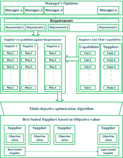
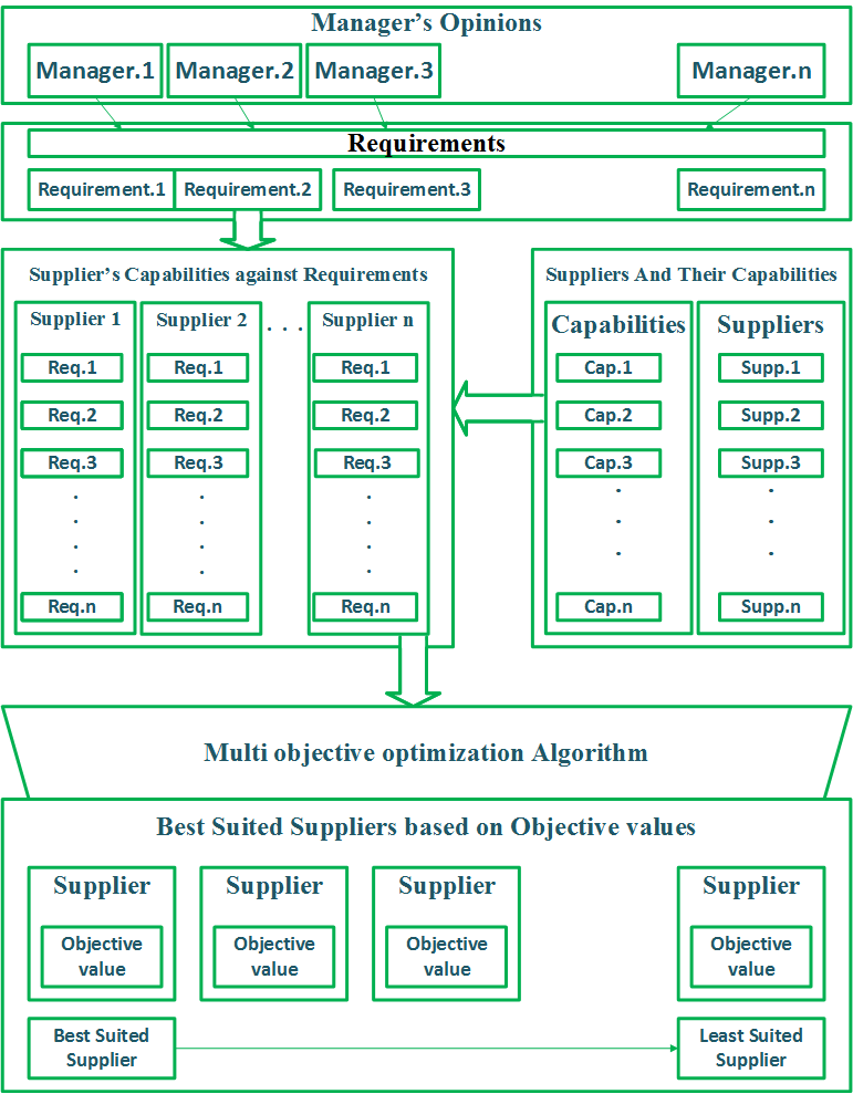
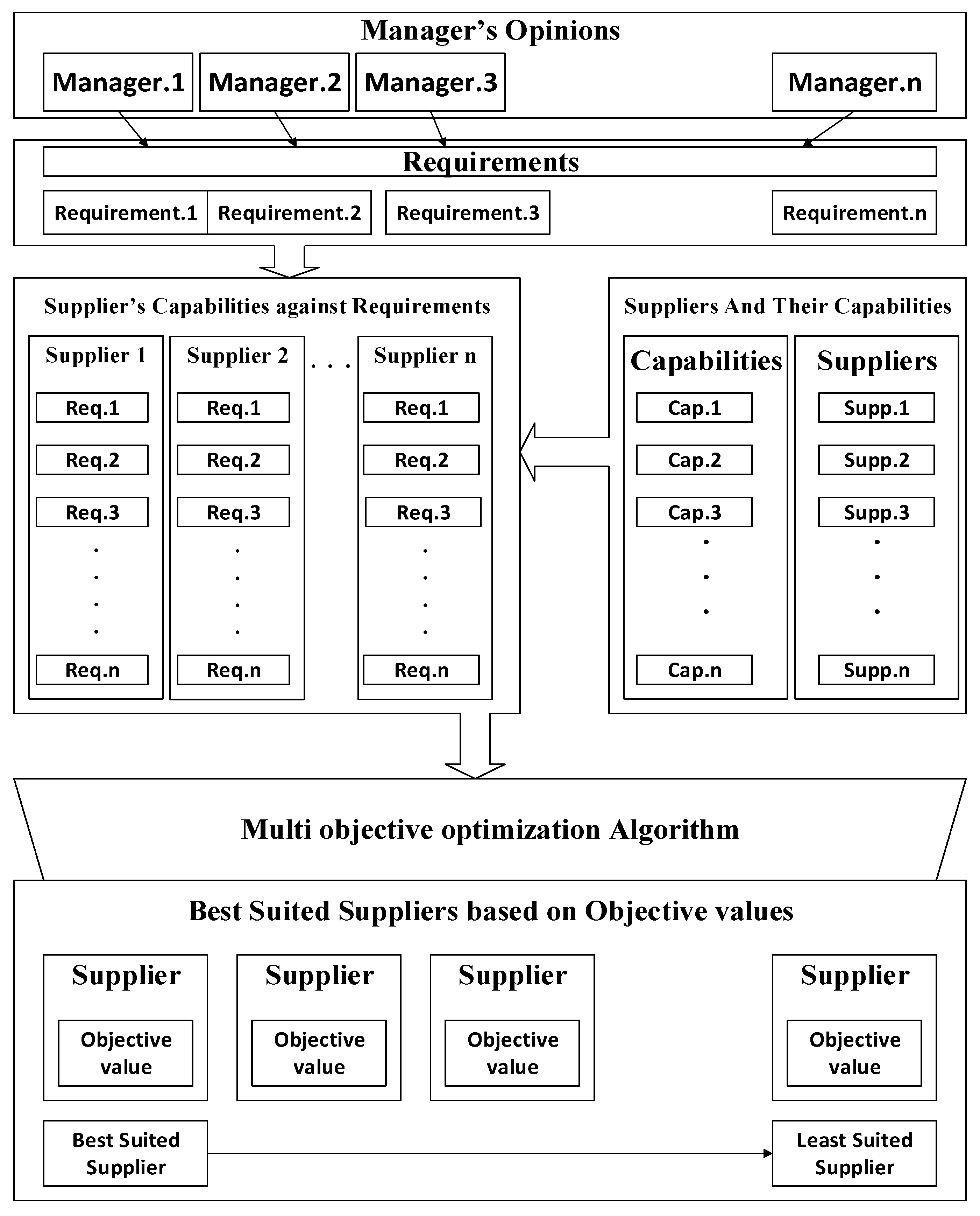
4. Proposed Framework

In this section, the developed ABC-based framework for SI is presented. The structure of the developed model consists of three layers, which are associated with the manager’s opinions, analysis of supplier capabilities against requirements, and the final decision making, in which selection is based on optimization through ABC. The three layers of the proposed SI model are described in the following sections and are shown in Figure 1.

4.1. Layer 1: Manager Opinions

The first layer of our model defines the industry requirements or the criteria that affect supplier selection decision, as suggested by the executive management in the industry or the experts from the field of SCM (supply chain management). Different factors are suggested by different managers and have diverse levels of importance. These factors serve as objectives in optimization modeling. The rating of these factors helps to achieve the optimum performance of the objective values. Basically, this layer rates each factor for use in the metaheuristic algorithms in the third layer. The rating of any factor $x$ by the i^th manger is represented as $x_i$, for $N$ opinions, where $i=1,\dots ,N.$

4.2. Layer 2: Supplier Capabilities

The second layer of this SI framework is the problem seeking layer, which helps an industry define its requirements for supplier development.

After obtaining the important opinions (requirements) from managers in the second layer, historical data were collected from the enterprise. These historical data consisted of the values of requirements/factors of different suppliers and constraints for integration with the suppliers. Objectives and constraints defined by the company were used as model inputs in the proper equations for mathematical optimization. Essentially, this layer helped to adjust all the requirements of the enterprise. The capabilities of each supplier were drawn against the requirements suggested by the experts. Each capability of the supplier was assigned a specific value based on the past performance of that specific supplier; this value was then used in the metaheuristic algorithm to find the most appropriate and best-suited supplier. Factors were treated as multi-objectives in this study, and they were treated in to two groups depending upon their nature. There were two main sets, i.e., maximization of desirable factors and minimization of undesirable factors. For maximization:

$$f_x=c_i{w}_{x}X\mathrm{Subject}\mathrm{to}\overline{r_x}\le X\le r_x$$

(1)

where c is the capacity of the supplier, $X$ is the desirable factor value for that supplier, w is the weight of the factor used, $r$ ris the upper limit of that factor, and $\overline{r}$ is the lower limit of that factor. Similarly, for minimization, Equation (2) is used:

$$f_{\overline{x}}=c_i{w}_{x}X\mathrm{Subject}\mathrm{to}\overline{r_x}\le X\le r_x$$

(2)

where, c is the capacity of the supplier, X is the factor value for that supplier, w is the weight of the factor used, $r$ is the upper limit of that factor, and $\overline{r}$ is the lower limit of that factor. However, we may convert the minimization function to a maximization function using Equation (3). The combined objective function is represented by Equation (4). In which A is availability of the supply from suppliers, $D$ is the demand of the firm, while s represents the number of suppliers to be ranked and S is the required number of suppliers by the firm to integrate:

$$f_x=1-f_{\overline{x}}\mathrm{subject}\mathrm{to}\overline{r_x}\le X\le r_x$$

(3)

$$\begin{gathered} Max:F\left(X\right)=f_{1\left(x\right)},f_{2\left(x\right)},\dots f_{i\left(x\right)} \\ Subject to: \overline{r_x}\le X\le r_x \\ A\ge D and s=S \end{gathered}$$

(4)

4.3. Layer 3: Multi Objective Optimization

On the bases of these opinions (requirements/ suggestions/ factors) in the second layer, the past performance data of suppliers were collected, and an analysis was performed using the optimization algorithm in the third layer. This layer analyzed the capabilities of all the given suppliers against all requirements suggested by the managers. The past data of suppliers, i.e., values against factors from layer 2, were used to identify the most appropriate supplier. To make this framework more flexible, a change in objectives was allowed, such that any firm may change the objective according to its need. A combined objective function was formulated to evaluate the suppliers. Therefore, all the factors were used in this combined objective function. All vendors were evaluated individually on the basis of this objective function. Basically, the effectiveness of each supplier was assessed with respect to all these objectives. Metaheuristic algorithms used these values to output priority based on the best-suited suppliers, considering all objective values and constraints. The process began with initialization using Equation (5). This essentially acts like a worker bee that produces a change in position (solution) in memory depending on local information (visual information) and tests the amount of nectar (value) of the new source of fitness (new solution):

$$x_{ij}=x_{j\min }+rand[1,0](x_{j\max }-x_{j\min })$$

(5)

Initially, random solutions were generated from the given data. These solutions were further used to determine the most appropriate solution. After the generation of initial random solutions, the probability of each solution was calculated to indicate the optimal solutions. Then, a probability check was performed using a probabilistic equation, i.e., Equation (6). This process acts like an onlooker bee, evaluating the information of nectar of all working bees and choosing a food source with a probability of a high quantity of nectar, where SN is the n^th solution:

$$p_i=\frac{fi{t}_i}{{\displaystyle {\sum }_{n=1}^{SN}fi{t}_n}}$$

(6)

Solutions in the previous steps were stored, and the more random solutions were generated as fitness values in the neighborhood of the optimum of the initially generated random values. This process helped to optimize the final solutions. After this probability check, random solutions are again generated using Equation (7):

$$v_{ij}=x_{ij}+{\varnothing }_{ij}(x_{ij}-x_{kj})$$

(7)

where $v_{ij}$ is the new solution, and $x_{ij}$ is the old or previous solution. After finally using the objective function, each supplier was evaluated. After the random search and probability check, we used our constraints and objective function to obtain our final solution. The last step essentially followed the case of the scout bee, which produces a change in position in its memory and checks for an even greater quantity of nectar. With identification of a new maximum, this bee stores the new position and forgets the previous.

In the developed framework, any enterprise can be used as a case study or problem, and unique data are then taken from that enterprise.

5. Data-Specific Solutions of the Framework

In this section, the previously modeled framework is implemented with a real-world problem of an actual manufacturing SME in Pakistan. The company’s manufacturing facility, situated near the city of Sialkot, produces different types of sports equipment including footballs, gloves, shin pads, etc. Production of these items solely depends upon a variety of raw materials supplied by different vendors, thus requiring long-term sustainable business relationships. The company is currently working with 10 different suppliers. The top management of the company wants a methodical prioritization of these suppliers based on their compatibility with the current and future production needs of the company so that it may shortlist some of these companies for long-term integration. Therefore, the problem lies within the domain of multi-objective optimization, which is the central methodology of our presented framework.

The first step of our framework is exploration and prioritization of all the factors, which can affect the SI decision. During the factor-prioritization phase of this study, a total of 400 questionnaires were distributed among the top management experts of 30 different SMEs of Pakistan. Out of these distributed questionnaires, 242 were returned to the authors. The questionnaires contained a rating scale for each of the factors with a range of 1 to 5, taking ‘1′ as the least significant and ‘5′ as the most significant. An average (arithmetic mean) was then calculated to assign absolute weights for all the factors. The factors Quality, Delivery, Costs, and Technical capability were computed as the most crucial, having weights of 4.78, 4.51, 4.33, and 4.24, respectively. As a next step, the performance of the selected suppliers was evaluated based on their previous performance with respect to the screened out factors.

This performance data was then utilized to implement the developed algorithm for further analysis. The past performance or historical data of the ten suppliers currently in business relations with the company are compiled in

Table 2. Weighted Factors.

Factors	Quality	Delivery	Cost	Technical Capability
Weightage	4.78	4.51	4.33	4.24

.

These data are related to the past two-year performance of these 10 main vendors where the ranges for all factors are expressed as percentages. The approximate demand of the company is about 200 units per month. The capacity of each supplier to meet this monthly demand is also presented. The company wants to select a maximum of four suppliers for long-term business integration. The ranges of the factors are given in

Table 3. Past Data.

Past Data of 10 Main Suppliers
Factors (Recommended Range in %)	Ranges of the Factors Against Vendors
Quality	80–90	90–95	85–90	85–90	80–90	60–75	60–70	80–90	85–90	85–95
Cost	40–48	60–70	30–40	40–45	55–60	25–30	30–35	45–50	25–35	35–45
Lead Time	80–85	85–95	60–65	65–70	65–70	90–95	80–85	85–90	75–80	85–90
Financial Position	70–85	65–70	80–85	90–95	95–100	60–70	60–70	80–90	80–95	90–95
Technical Capability	60–75	25–35	30–40	15–20	30–35	35–40	20–25	30–40	20–30	30–35
After Sale Support	80–85	60–65	80–90	70–85	60–70	60–65	70–80	90–95	65–70	90–95
Relationships	85–90	90–95	85–90	80–85	85–90	85–90	85–90	90–95	70–75	90–95
Delivery	90–95	85–90	85–90	90–95	80–85	85–90	75–85	90–95	80–90	95–100
Supplier number	1	2	3	4	5	6	7	8	9	10
Capacity of Supplier (Units/month)	50	63	75	55	50	43	38	56	65	72

. The data-specific problem was solved using the proposed AABC algorithm. The results were further validated using basic ABC algorithm and particle swarm optimization (PSO) algorithm. The results obtained from the simulation are presented in the next section. The proposed AABC algorithm is shown in Figure 2.

6. Results and Discussion

In this section, the results obtained from the simulation of metaheuristic algorithms, proposed in the third layer of our SI framework, are discussed for different scenarios. We used MATLAB (MIT, R2017b, Natick, MA, USA) for performing the experiments. The simulation parameters used in the entire experimentation process are shown in

Table 4. Simulation parameters.

Parameter	Value
Maximum number of cycles	50
Number of food sources	10
Demand limit	200

.

Since Quality has the maximum weight and importance, followed by Delivery and Costs, the suppliers stronger in these three factors secured the top positions in the priority list generated by the simulations of the algorithms. The results show that suppliers 10, 3, and 2 were the most suitable and meet the demands of the company; therefore, they are optimum alternatives. On the contrary, suppliers 1, 7, and 5 were computed to be the least suitable options as they achieved lower scores from the ABC simulation for the above-mentioned critical factors. The results clearly showed that the best-suited algorithm for this problem is the AABC algorithm.

It achieved quick convergence towards the optimal value in 35^th cycle with an objective function value of 65,000. However, to ensure avoidance of not getting trapped in local optima, 60 cycles were run. Following the AABC algorithm, the original ABC approach demonstrated good results and achieved near-optimal solution in a short period of time; to be more specific, 650,000 in 45^th cycle and remained steady until termination. Finally, the PSO algorithm did not effectively achieve an optimum solution on this SI problem, and its performance was slower than those of the AABC and the original ABC algorithm, as it only attained its maximum objective value at its 50^th cycle, which is far less than the one achieved by AABC. Results obtained from the AABC, ABC, and PSO approaches are plotted in Figure 3.

Analysis of Variance (ANOVA) was conducted on 60 separate runs of each algorithm: ABC, AABC, and PSO to validate it statistically. In

Table 5. ANOVA Results for ABC, AABC, and PSO.

Source	Degree of Freedom (DF)	Adj SS	Adj MS	F-Value	P-Value
Factor	2	4.06532 $\times$ 1011	2.03266 $\times$ 1011	201.93	0.000
Error	147	1.47973 $\times$ 1011	10 $\times$ 106
Total	149	5.54505 $\times$ 1011

, results from ANOVA are presented, and this test proves to be significant, as the p value is less than 0.05, which depicts that performance of the three algorithms differs. To further explore that which algorithm differed significantly, a Tukey post hoc test was conducted as shown in Figure 4. The Tukey test showed that ABC-PSO and AABC-PSO varied significantly, while AABC was in good agreement. However, the Box plot shown in Figure 5 was inculcated to further validate the better performance of AABC statistically, distinguishing it from ABC through better performance. Figure 5, depicts the visual summarization of the data acquired from the result of the three algorithms deployed in the current research. It is clear from Figure 5 that the median of PSO is the lowest and ABC has more data points between interquartile. While AABC achieves optimized value although with a somehow larger data spread, it would still be based on the decision maker to achieve the best optimized result or have a reduced data spread with sub-optimal result.

A sensitivity analysis was performed by varying the importance levels of the factors to access the responses of implemented algorithms. Thus, different hypothetical scenarios were generated while varying the requirements of the company. This analysis helps us to observe the impact of changing inputs on the final decision. The scenarios are presented in Figure 6.

Scenario 1 (Quality): in this hypothetical scenario, quality is set to the maximum importance and weight by minimizing other factors. Quality represents the standard of the raw material provided by different suppliers. This scenario shows that supplier number 2, 3, and 10 are the best at meeting the demand of company for quality at a 95% level. These suppliers produce better raw material compared with the others and also meet the constraints defined by the company.

Scenario 2 (Cost): high cost is an undesirable factor and should be minimized from the company’s business point of view. Suppliers with minimum cost, if they meet the other limitation constraints, should be preferred over the others. When the cost is assigned the highest level of importance, supplier number 3, supplier number 6, and supplier number 9 are the optimal alternatives.

Other Scenarios: similarly, scenarios for all the eight factors were run one by one and the results are represented in Figure 6. In each case, the factor considered as most crucial is highlighted in the box, whereas the three best suppliers against this factor, as computed by the ABC simulation, are shown in the decision box.

7. Conclusions

This paper proposes a framework that is composed of an archived artificial bee colony algorithm, based on multi-objective optimization. The factors affecting these supplier selection decisions were screened from the relevant literature under the guidance of industry experts to ensure suitability with respect to the current environment of the selected country. Implementation of a developed AABC-based SI framework provided highly meaningful and beneficial results for the concerned SME, since it is based on simulation of scientifically accepted optimization techniques. This study concludes that, when choosing alternatives for integration, experts of the selected SME in Pakistan gave the highest preference to factors such as quality, delivery, and costs. In contrast, they were not very concerned about the financial positions of the suppliers or their previous relationships. In light of these assigned priorities and based on the factual quantitative data of the 10 suppliers, the simulation showed that the alternatives stronger in these key factors can be declared the best, despite that they are often weak with respect to other factors, such as financial position. A detailed and in-depth evaluation of suppliers was provided by the sensitivity analysis, which presented a more rigorous authentication and elaboration of the results. The presented framework is the first of its kind for the SMEs of Pakistan and can be applied with little modification to other industries.

References

1. Ghodsypour, S.H.; O’Brien, C. A decision support system for supplier selection using an integrated analytic hierarchy process and linear programming. Int. J. Prod. Econ. 1998, 1, 199–212. [Google Scholar] [CrossRef]
2. Locatelli, G.; Mancini, M.; Ishimwe, A. How can system engineering improve supplier management in megaprojects? Procedia Soc. Behav. Sci. 2014, 119, 510–518. [Google Scholar] [CrossRef]
3. So, S.; Sun, H. Supplier integration strategy for lean manufacturing adoption in electronic-enabled supply chains. Supply Chain Manag. Int. J. 2010, 15, 474–487. [Google Scholar] [CrossRef]
4. Petersen, K.J.; Handfield, R.B.; Ragatz, G.L. A model of supplier integration into new product development. J. Prod. Innov. Manag. 2003, 20, 284–299. [Google Scholar] [CrossRef]
5. Ylimäki, J. A dynamic model of supplier–customer product development collaboration strategies. Ind. Mark. Manag. 2014, 43, 996–1004. [Google Scholar] [CrossRef]
6. Huikkola, T.; Ylimäki, J.; Kohtamäki, M. Joint learning in R&D collaborations and the facilitating relational practices. Ind. Mark. Manag. 2013, 42, 1167–1180. [Google Scholar]
7. Distel, S.; Klaus, P.; Prockl, G.; Baresel, A.; Zimmermann, R. Integrated Supplier—ECR is Also for Suppliers of Ingredients, Raw Materials and Packaging; Efficient Consumer Response Europe: Munich, Germany, 2000. [Google Scholar]
8. Lockström, M.; Schadel, J.; Harrison, N.; Moser, R.; Malhotra, M.K. Antecedents to supplier integration in the automotive industry: A multiple-case study of foreign subsidiaries in China. J. Oper. Manag. 2010, 28, 240–256. [Google Scholar] [CrossRef]
9. Bercz, C. Supplier Integration Systems: Understanding Adoption Process and Structure. Master’s Thesis, University of Twente, Enschede, The Netherlands, 2008. [Google Scholar]
10. Danese, P.; Romano, P.; Vinelli, A. Managing business processes across supply networks: The role of coordination mechanisms. J. Purch. Supply Manag. 2004, 10, 165–177. [Google Scholar] [CrossRef]
11. Dou, Y.; Zhu, Q.; Sarkis, J. Evaluating green supplier development programs with a grey-analytical network process-based methodology. Eur. J. Oper. Res. 2014, 233, 420–431. [Google Scholar] [CrossRef]
12. Talluri, S.; Sarkis, J. A model for performance monitoring of suppliers. Int. J. Prod. Res. 2002, 40, 4257–4269. [Google Scholar] [CrossRef]
13. Huang, S.H.; Keskar, H. Comprehensive and configurable metrics for supplier selection. Int. J. Prod. Econ. 2007, 105, 510–523. [Google Scholar] [CrossRef]
14. Liker, J.K.; Choi, T.Y. Building deep supplier relationships. Harv. Bus. Rev. 2004, 82, 104–113. [Google Scholar]
15. Hartley, J.L.; Choi, T.Y. Supplier development: Customers as a catalyst of process change. Bus. Horiz. 1996, 39, 37–44. [Google Scholar] [CrossRef]
16. Verma, R.; Pullman, M.E. An analysis of the supplier selection process. Omega 1998, 26, 739–750. [Google Scholar] [CrossRef]
17. Goh, S.H.; Eldridge, S. New product introduction and supplier integration in sales and operations planning: Evidence from the Asia Pacific region. Int. J. Phys. Distrib. Logist. Manag. 2015, 45, 861–886. [Google Scholar] [CrossRef]
18. Kotula, M.; Ho, W.; Dey, P.K.; Lee, C.K.M. Strategic sourcing supplier selection misalignment with critical success factors: Findings from multiple case studies in Germany and the United Kingdom. Int. J. Prod. Econ. 2015, 166, 238–247. [Google Scholar] [CrossRef] [Green Version]
19. Banaeian, N.; Mobli, H.; Fahimnia, B.; Nielsen, I.E.; Omid, M. Green supplier selection using fuzzy group decision making methods: A case study from the agri-food industry. Comput. Oper. Res. 2018, 89, 337–347. [Google Scholar] [CrossRef]
20. Memon, M.S.; Mari, S.I.; Shaikh, F.; Shaikh, S.A. A grey-fuzzy multiobjective model for supplier selection and production-distribution planning considering consumer safety. Math. Probl. Eng. 2018, 2018, 17. [Google Scholar] [CrossRef]
21. Alkahtani, M. Automobile tire assessment: A multi-criteria approach. Eng. Technol. Appl. Sci. Res. 2016, 7, 1363–1368. [Google Scholar]
22. Humphreys, P.K.; Li, W.; Chan, L. The impact of supplier development on buyer–supplier performance. Omega 2004, 32, 131–143. [Google Scholar] [CrossRef]
23. Dai, J.; Blackhurst, J. A four-phase AHP–QFD approach for supplier assessment: A sustainability perspective. Int. J. Prod. Res. 2012, 50, 5474–5490. [Google Scholar] [CrossRef]
24. Ağan, Y.; Kuzey, C.; Acar, M.F.; Açıkgöz, A. The relationships between corporate social responsibility, environmental supplier development, and firm performance. J. Clean. Prod. 2014, 112, 1872–1881. [Google Scholar] [CrossRef]
25. Shad, Z.; Roghanian, E.; Mojibian, F. Integration of QFD, AHP, and LPP methods in supplier development problems under uncertainty. J. Ind. Eng. Int. 2014, 10, 1–9. [Google Scholar] [CrossRef]
26. Sancha, C.; Longoni, A.; Giménez, C. Sustainable supplier development practices: Drivers and enablers in a global context. J. Purch. Supply Manag. 2015, 21, 95–102. [Google Scholar] [CrossRef]
27. Ekhtiari, M.; Poursafary, S. Multiobjective stochastic programming for mixed integer vendor selection problem using artificial bee colony algorithm. ISRN Artif. Intell. 2013, 2013, 13. [Google Scholar] [CrossRef]
28. Karaboga, D.; Akay, B. A comparative study of artificial bee colony algorithm. Appl. Math. Comput. 2009, 214, 108–132. [Google Scholar] [CrossRef]
29. Ilgin, M.A.; Gupta, S.M. Environmentally manufacturing and product recovery (ECMPRO): A review of the state of the art. J. Environ. Manag. 2010, 91, 563–591. [Google Scholar] [CrossRef] [PubMed]
30. Gupta, S.M.; Gungor, A. Product recovery using a disassembly line: Challenges and solution. In Proceedings of the 2001 IEEE International Symposium on Electronics and the Environment, Denver, CO, USA, 9 May 2001; pp. 36–40. [Google Scholar]
31. Koc, A.; Sabuncuoglu, I.; Erel, E. Two exact formulations for disassembly line balancing problems with task precedence diagram construction using an AND/OR graph. IIE Trans. 2009, 41, 866–881. [Google Scholar] [CrossRef]
32. Altekin, F.T.; Akkan, C. Task-failure-driven rebalancing of disassembly lines. Int. J. Prod. Res. 2012, 50, 4955–4976. [Google Scholar] [CrossRef]
33. Bentaha, M.L.; Battaia, O.; Dolgui, A. A sample average approximation method for disassembly line balancing problem under uncertainty. Comput. Oper. Res. 2014, 51, 111–122. [Google Scholar] [CrossRef]
34. Altekin, F.T.; Kandiller, L.; Ozdemirel, N.E. Profit-oriented disassembly-line balancing. Int. J. Prod. Res. 2008, 46, 2675–2693. [Google Scholar] [CrossRef] [Green Version]
35. Mcgovern, S.M.; Gupta, S.M. Combinatorial optimization analysis of the unary NP-complete disassembly line balancing problem. Int. J. Prod. Res. 2007, 45, 4485–4511. [Google Scholar] [CrossRef]
36. Mcgovern, S.M.; Gupta, S.M. A balancing method and genetic algorithm for disassembly line balancing. Eur. J. Oper. Res. 2007, 179, 692–708. [Google Scholar] [CrossRef]
37. Yang, H.; Zeqiang, Z.; Wang Kaipu, W.; Lili, M. Pareto bacterial foraging algorithm for multi-objective disassembly line balance problem. J. Comput. Appl. 2016, 33, 3265–3269. [Google Scholar]
38. Ding, L.-P.; Feng, Y.-X.; Tan, J.-R.; Gao, Y.-C. A new multi-objective ant colony algorithm for solving the disassembly line balancing problem. Int. J. Adv. Manuf. Technol. 2010, 48, 761–771. [Google Scholar] [CrossRef]
39. Ming, L.; Zeqiang, Z.; Yang, H. Research on disassembly line balance problem and its solving algorithm for U-shaped layout. Mod. Manuf. Eng. 2015, 7, 7–12. [Google Scholar]
40. Kalayci, C.B.; Hancilar, A.; Gungor, A.; Gupta, S.M. Multi-objective fuzzy disassembly line balancing using a hybrid discrete artificial bee colony algorithm. J. Manuf. Syst. 2015, 37, 672–682. [Google Scholar] [CrossRef] [Green Version]
41. Scholl, A.; Boysen, N.; Fliedner, M. The sequence-dependent assembly line balancing problem. OR Spectr. 2008, 30, 579–609. [Google Scholar] [CrossRef]
42. Andrés, C.; Miralles, C.; Pastor, R. Balancing and scheduling tasks in assembly lines with sequence-dependent setup times. Eur. J. Oper. Res. 2008, 187, 1212–1223. [Google Scholar] [CrossRef] [Green Version]
43. Yolmeh, A.; Kianfar, F. An efficient hybrid genetic algorithm to solve assembly line balancing problem with sequence-dependent setup times. Comput. Ind. Eng. 2012, 62, 936–945. [Google Scholar] [CrossRef]
44. Hamta, N.; Ghomi, S.M.T.F.; Jolai, F.; Shirazi, M.A. A hybrid PSO algorithm for a multi-objective assembly line balancing problem with flexible operation times, sequence-dependent setup times and learning effect. Int. J. Prod. Econ. 2013, 141, 99–111. [Google Scholar] [CrossRef]
45. Akpinar, S.; Bayhan, G.M.; Baykasoglu, A. Hybridizing ant colony optimization via genetic algorithm for mixed-model assembly line balancing problem with sequence dependent setup times between tasks. Appl. Soft Comput. 2013, 13, 574–589. [Google Scholar] [CrossRef]
46. Kalayci, C.B.; Gupta, S.M. Ant colony optimization for sequence-dependent disassembly line balancing problem. J. Manuf. Technol. Manag. 2013, 24, 413–427. [Google Scholar] [CrossRef]
47. Kalayci, C.B.; Polat, O.; Gupta, S.M. A hybrid genetic algorithm for sequence-dependent disassembly line balancing problem. Ann. Oper. Res. 2016, 242, 321–354. [Google Scholar] [CrossRef]
48. Kalayci, C.B.; Gupta, S.M. A tabu search algorithm for balancing a sequence-dependent disassembly line. Prod. Plan. Control 2014, 25, 149–160. [Google Scholar] [CrossRef]
49. Kalayci, C.B.; Polat, O.; Gupta, S.M. A variable neighbourhood search algorithm for disassembly lines. J. Manuf. Technol. Manag. 2015, 26, 182–194. [Google Scholar] [CrossRef]
50. Kalayci, C.B.; Gupta, S.M. Artificial bee colony algorithm for solving sequence-dependent disassembly line balancing problem. Expert Syst. Appl. 2013, 40, 7231–7241. [Google Scholar] [CrossRef]
51. Özbakir, L.; Baykasoğlu, A.; Tapkan, P. Bees algorithm for generalized assignment problem. Appl. Math. Comput. 2010, 215, 3782–3795. [Google Scholar] [CrossRef]
52. Fahmy, A. Using the Bees Algorithm to select the optimal speed parameters for wind turbine generators. J. King Saud Univ. Comput. Inf. Sci. 2012, 24, 17–26. [Google Scholar] [CrossRef] [Green Version]
53. Yuce, B.; Packianather, M.S.; Mastrocinque, E.; Pham, D.T.; Lambiase, A. Honey bees inspired optimization method: The Bees Algorithm. Insects 2013, 4, 646–662. [Google Scholar] [CrossRef] [PubMed]
54. Delgado-Osuna, J.A.; Lozano, M.; García-Martínez, C. An alternative artificial bee colony algorithm with destructive–constructive neighbourhood operator for the problem of composing medical crews. Inf. Sci. 2016, 326, 215–226. [Google Scholar] [CrossRef]
55. Pham, D.; Ghanbarzadeh, A. Multi-objective optimisation using the Bees Algorithm. In Proceedings of the 3rd IPROMS Conference, Cardiff, UK, 2–13 July 2007. [Google Scholar]
56. Karaboga, D.; Ozturk, C. A novel clustering approach: Artificial Bee Colony (ABC) algorithm. Appl. Soft Comput. 2011, 11, 652–657. [Google Scholar] [CrossRef]
57. Bouaziz, A.; Draa, A.; Chikhi, S. Artificial bees for multilevel thresholding of iris images. Swarm Evolut. Comput. 2015, 21, 32–40. [Google Scholar] [CrossRef]
Figure 1. Proposed supplier integrations (SI) Framework.
Applsci 09 00588 g001
Figure 2. A flowchart of the proposed archived artificial bee colony (AABC) algorithm.
Applsci 09 00588 g002
Figure 3. Algorithm Comparison in SI Optimization.
Applsci 09 00588 g003
Figure 4. Tucky Test at 95% confidence interval (CI).
Applsci 09 00588 g004
Figure 5. Box Plot for Algorithms Results.
Applsci 09 00588 g005
Figure 6. Sensitivity Analysis.
Applsci 09 00588 g006