Slope Failure of Noncohesive Media Modelled with the Combined Finite–Discrete Element Method

Abstract

Slope failure behaviour of noncohesive media with the consideration of gravity and ground excitations is examined using the two-dimensional combined finite–discrete element method (FDEM). The FDEM aims at solving large-scale transient dynamics and is particularly suitable for this problem. The method discretises an entity into a couple of individual discrete elements. Within each discrete element, the finite element method (FEM) formulation is embedded so that contact forces and deformation between and of these discrete elements can be predicted more accurately. Noncohesive media is simply modelled with assembly of individual discrete elements without cohesion, that is, no joint elements need to be defined. To validate the effectiveness of the FDEM modelling, two examples are presented and compared with results from other sources. The FDEM results on gravitational collapse of rectangular soil heap and landslide triggered by the Chi-Chi earthquake show that the method is applicable and reliable for the analysis of slope failure behaviour of noncohesive media through comparison with results from other known methods such as the smoothed particle hydrodynamics (SPH), the discrete element method (DEM) and the material point method (MPM).

1. Introduction

Slope failure, including rock slide and landslide, is particularly detrimental and hazardous to human lives and engineering infrastructures [1]. Therefore, much attention has been paid to the slope stability analysis from geotechnical communities during the past decades. Generally, slope failure is caused by instability triggered by internal or external factors. Among all these factors, earthquake excitation [2] and rainfall [3] have been recognised as major causes. Apart from the triggering of slope instability, the inherent failure mechanism, failure process and postfailure behaviour are also of significance.

Methods used to investigate slope instability can be categorised as experimental and numerical. Researchers used to conduct shaking table tests and other experimental approaches to investigate the failure of slopes [4,5]. Though experimental studies are direct, they are expensive and time-consuming, and it is not easy to perform large-scale parametric studies. Consequently, numerical modelling has become popular in recent decades.

There are a number of numerical methods that can be employed to examine the slope instability and the failure process. Since discontinuous and large displacements are involved in slope failure, traditional finite element method (FEM) is not best suited for this sort of analysis. It is argued that the discrete element method (DEM) is naturally accommodated for discontinuous problems. Choi and Chung [6] analysed the stability of jointed rock slopes using explicit DEM UDEC. In reference [7], Wu et al. employed an implicit discontinuous deformation analysis (DDA) for the dynamic analysis of a slope in the Taiwan Chi-Chi earthquake. Other computational methods contributing to the development of slope stability analysis include the material point method (MPM) [8,9], the smoothed particle hydrodynamics (SPH) [4,5], the meshless method [10,11] and the extended finite element method (XFEM) [12].

In this study, the two-dimensional combined finite–discrete element method (FDEM) is employed. The FDEM is a special branch of the DEM. It aims at solving large-scale transient dynamics where discontinuous entities and multiple contacts are involved. The method has been developed since the 1990s [13,14]. In the FDEM, each element is a discrete element. Within each discrete element, finite element mesh is embedded and thus more accurate evaluation of contact forces and deformation becomes possible. Details on the FDEM can be referred to in the monographs of Munjiza and his coworkers [15,16,17]. The FDEM has been employed in a variety of brittle and quasi-brittle materials in recent years [18,19,20]. Regarding slope failure modelling of noncohesive media with the FDEM, MR contact detection is a very important aspect to determine whether element pairs are in contact or not. Further details on the MR contact detection algorithm can be referred to [16,21]. Previous work on geotechnical considerations with the FDEM is traceable. A simple rock fall problem under gravity was given in reference [22] for the illustration purpose of the Y-GUI. Piovano et al. [23] simulated the instability of a homogeneous slope along a circular sliding surface under gravity with the FDEM. Their results were compared with those from limit equilibrium method (LEM) and FEM, and factor of safety was calculated. Grasselli et al. [24] performed slope stability analysis using the FDEM, and presented examples including rock fall, toppling failure, cliff recession and planar slide. However, geometries of these given examples were simple and regular. Later, algorithmic developments [25] were included into the Y-Geo code which is based on the FDEM. Examples on cliff recession were presented, and emphasis was given to the fracture and failure of rocks. Recently, Feng et al. [26] examined the stability of an ancient slope in western Beijing, China, under gravity with the FDEM, and compared their results with field surveys.

Although there are some research endeavours conducted on rock or slope failure using the FDEM, seismic failure behaviour of slope media has not been prevalently included in the work aforementioned. Furthermore, quantitative comparison with existing literature is still high in demand. This paper focuses on the slope failure behaviour of noncohesive media considering both gravity and seismic excitations. In this study, nonparallel 2D FDEM program ‘Y’, which was implemented by Munjiza [27], is used for the simulation. Computational work was performed on a Dell T7910 workstation with Intel Xeon E5-2630v4 2.2 GHz CPU, 32 GB memory and Microsoft Windows 10 operating system. Following the basics of the FDEM, two examples on noncohesive slope failure are given. One example is the collapse of a rectangular soil heap under gravity, and the other simulates a landslide disaster triggered by the 1999 Taiwan Chi-Chi earthquake. The noncohesive media is discretised into a number of discrete elements, and no further fracture of these discrete elements is considered. Results are compared and validated both qualitatively and quantitatively with data in existing literature. It is worth mentioning that the effect of water is not considered in this study, suggesting the slope media is well drained. This assumption is widely held and accepted in a good number of cases. In general, the combined FDEM is proven to be an applicable and reliable computational tool for modelling slope failure of noncohesive media.

2. Method and Modelling

In this section, the combined FDEM is briefly introduced. Some basics of the FDEM are addressed, and further details can be referred to [15]. In the FDEM, motions of elements are determined by traditional DEM equations. Translational and rotational motions of a single discrete element i is predicted from Newton’s second law:

$$m_i\frac{d^2}{d{t}^2}{r}_i=F_i$$

(1)

$$I_i\frac{d}{dt}{\omega }_i=T_i$$

(2)

where m_i is the mass of element i; r_i is the position; I_i is the moment of inertia; ω_i is the angular velocity; F_i and T_i are net external force and torque, respectively. Consequently, velocity and position of an arbitrary element can be obtained from Equations (1) and (2).

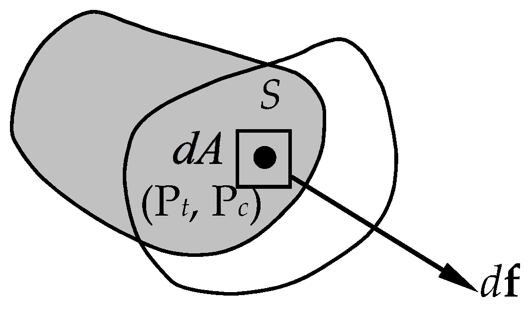
Contact forces in the FDEM are computed from the overlapping area S. Figure 1 shows two entities in contact. Infinitesimal contact force df exists in elemental penetration area dA, as:

$$d\mathrm{f}=-d{\mathrm{f}}_{\mathrm{t}}+d{\mathrm{f}}_{\mathrm{c}}$$

(3)

where subscripts ‘t’ and ‘c’ correspond to the target and contactor, respectively. df_t and df_c are defined as follows.

$$d{\mathbf{f}}_{\mathrm{t}}=-E_{p}grad{\phi }_c({\mathrm{P}}_c)dA$$

(4)

$$d{\mathbf{f}}_{\mathrm{c}}=-E_{p}grad{\phi }_t({\mathrm{P}}_t)dA$$

(5)

In Equations (4) and (5), P_c and P_t are points on contactor and target which share the same coordinate on S; φ_c and φ_t are predefined potentials; grad is the gradient and E_p is the contact penalty. Integrating dA over S, contact force f is obtained as:

$$\mathbf{f}=E_p{\displaystyle {\int }_S[grad{\phi }_c({\mathrm{P}}_c)-grad{\phi }_t({\mathrm{P}}_t)]}dA$$

(6)

Friction angle plays a role in the relationship between the shear strength and normal stress, as:

τ = σ tan(Φ) + c

(7)

where τ is the shear strength, σ is the normal stress, c is the cohesion and Φ is the angle of internal friction. In compression, σ should be replaced with −σ in Equation (7).

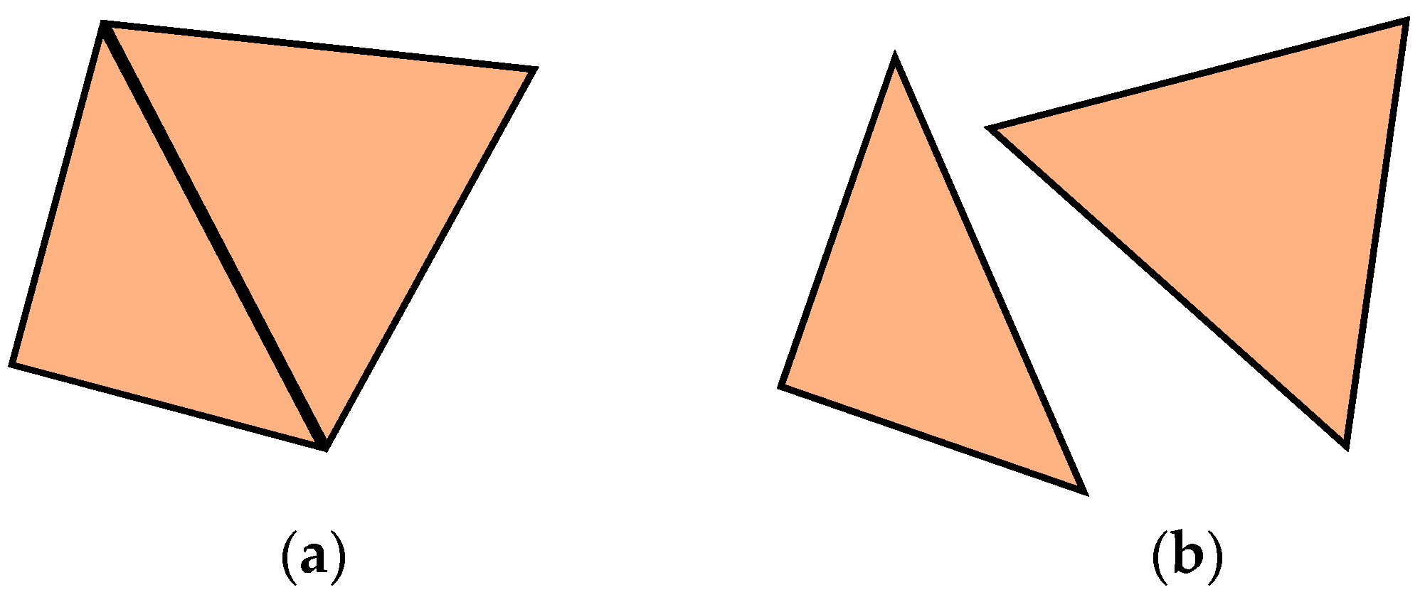
When modelling noncohesive media, no dummy joint elements are necessary to be accommodated between adjacent element pairs whose elements are initially in close contact. This suggests that the two elements are completely free and can naturally separate (see Figure 2). Only friction exists between their contact surfaces. It is worth mentioning that when modelling continua entities where fracture is not considered (e.g., steel frames or nonfailed mountain in following examples), any adjacent elements cannot separate.

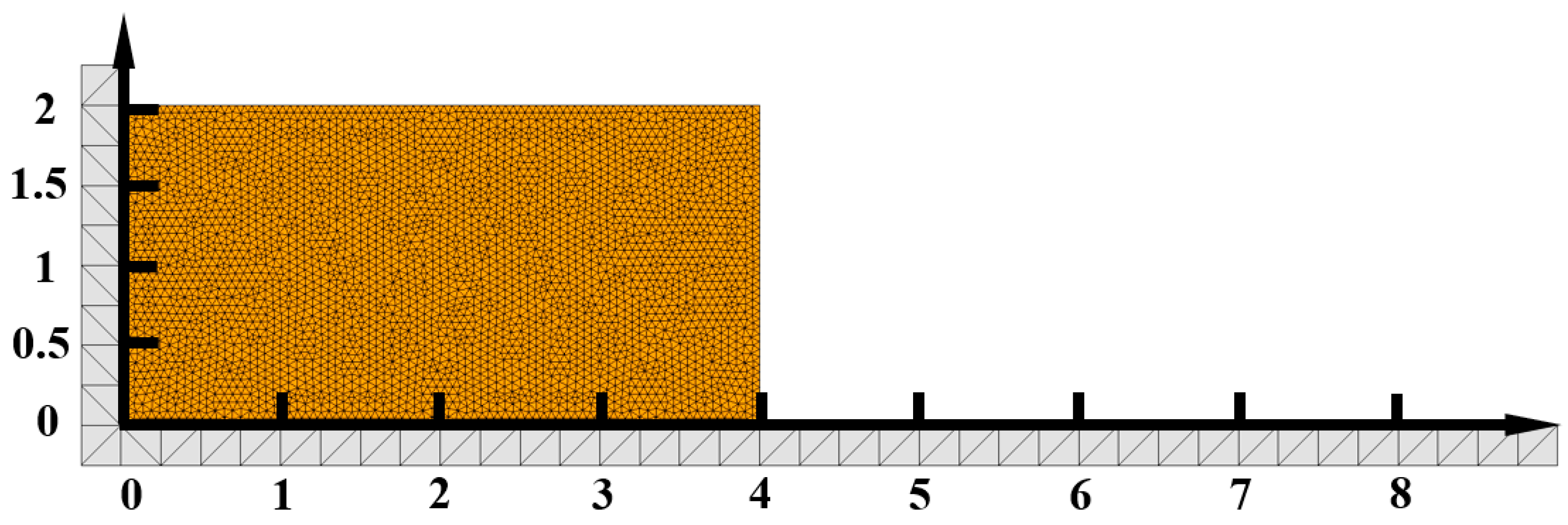
3. Example I: Rectangular Noncohesive Soil Heap under Gravity

In this example, an initially rectangular soil area (4 m × 2 m) subject to gravity is modelled with the FDEM (see Figure 3). It should be noted that in the current 2D FDEM program, only constant strain triangular (CST) elements are available, and thus entities are all meshed with triangular elements.

There are 7234 elements in total, with 7142 elements for rectangular soil heap and 92 elements for support. Characteristic element size for soil heap is 0.048 m. The support is made of steel. Soil and steel material parameters are given in

Table 1. Material properties of soil and steel.

Parameter	Soil	Steel
Young’s modulus (MPa)	1.8	200,000
Poisson’s ratio	0.3	0.3
Density (kg/m3)	1850.0	7800.0
Friction angle (°)	25	-

from reference [5]. Friction coefficient between soil–soil and soil–steel are defined as 0.6. The support is fixed and gravity (9.8 m/s²) is applied to the soil. Time step is 0.1 μs. Since the FDEM program used is nonparallel and the CPU frequency is not high, it costs 298.6 hours to bring the simulation to 2.5 s on the previously mentioned computer. However, the parallel version of the program with GPU acceleration is under testing and will come out soon.

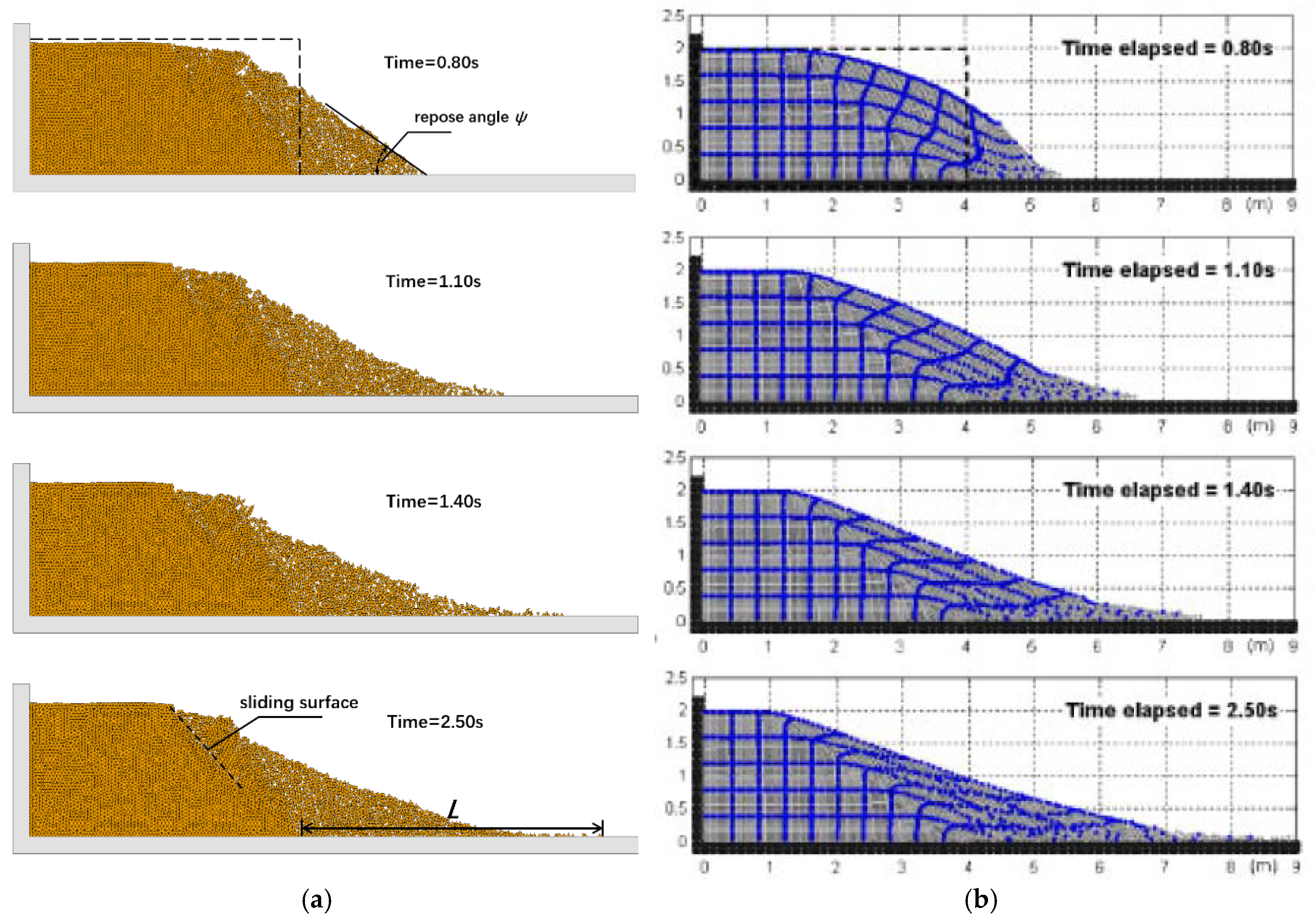
It is understood that since there is no support for the right side of the noncohesive soil, it will collapse naturally under gravity. Figure 4a shows the failure process of the soil at representative time points from the FDEM modelling. Corresponding results simulated by SPH [5] are given opposite in Figure 4b for comparison. It can be observed from Figure 4 that good agreement is reached. Large deformation and failure of soil have been well simulated out within the FDEM framework. Soil moves to the right and a repose angle ψ has been formed in the FDEM simulation. With the time elapsing, the angle of repose gets smaller. A summary on the repose angle is tabulated in

Table 2. Comparison on the repose angle at different time points.

Time (s)	Repose Angle ψ (°)
	FDEM	SPH
0.8	34	39
1.1	24	23
1.4	21	20
2.5	20	17

.

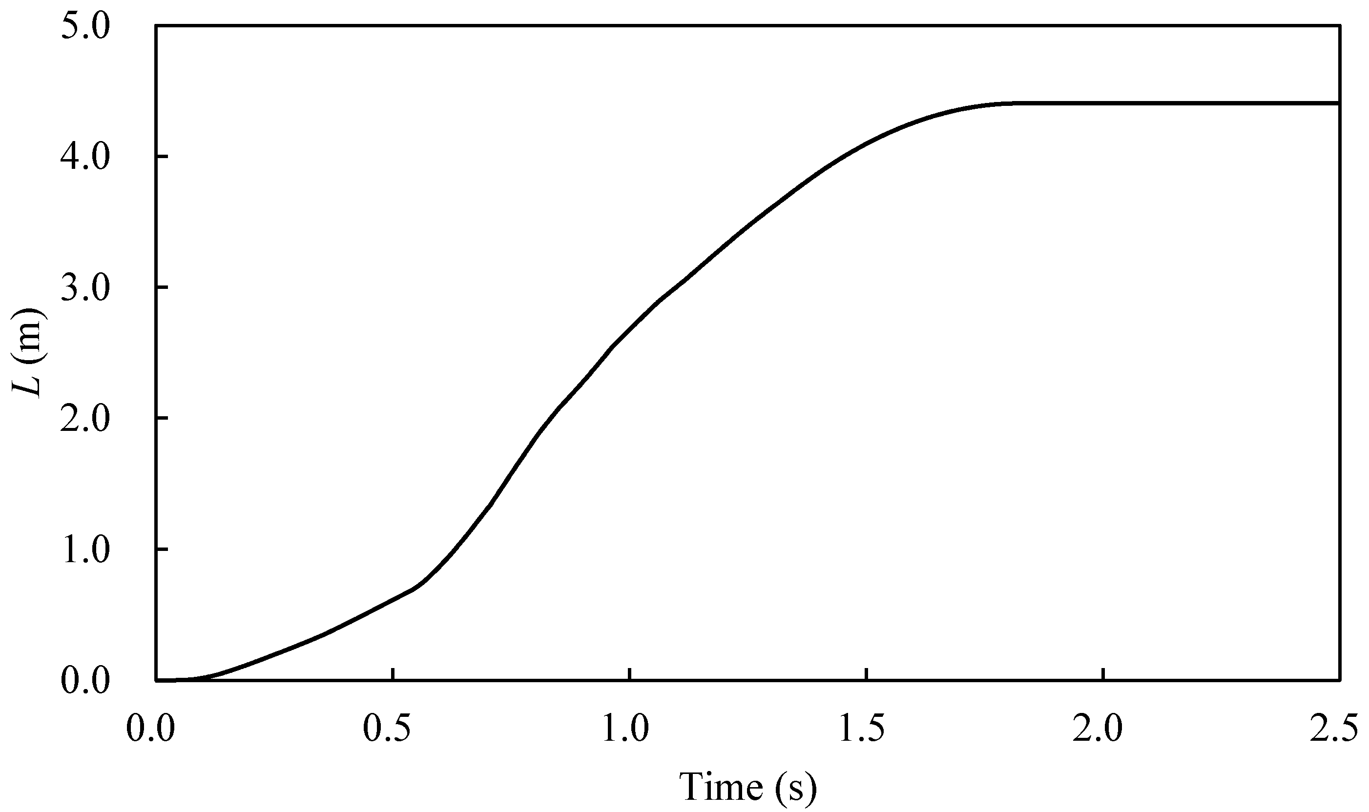
Besides the repose angle, failure processes produced by both the FDEM and the SPH agree with each other well. Since no cohesion is considered in the FDEM modelling, soil acts as granular material. At the early stage of the failure (t = 0.8 s), a steeper slope is formed with smaller horizontal distance L. Later, soil moves rightwards gradually and eventually rests after t = 1.8 s. A graph on the evolution of L versus time is plotted in Figure 5. Similar results were also obtained using the SPH, and the horizontal distance (L) that soil collapses to the right is close to that in the FDEM simulation. Through comparison, results of the FDEM modelling on noncohesive soil failure are highly consistent with those from SPH modelling. In spite of the consistency on the results from the two methods, the solid-mechanics-based FDEM has advantages over the SPH method which is based on hydrodynamics in simulating the behaviour of solid materials, like slope instability and dynamic sliding motion in this study. Moreover, engineering applications of SPH method are limited due to its own limitations, such as difficulty in setting boundary conditions and high computational cost.

4. Example II: Landslide Triggered by Chi-Chi Earthquake

The Chiu-fen-erh-shan landslide induced by the Chi-Chi earthquake which occurred in 1999 is examined in this section. Various methods have been employed for previous simulations [7,8]. Huge amount of rock mass high in the mountain travelled a long distance and deposited at the foot of the mountain. According to previous studies, the sliding rock masses are initially weak and disintegrated. Consequently, noncohesive rock blocks are used in the FDEM modelling. Once the rock masses are excited by the earthquake, they will fall along the mountain slope surface and mass flow can be formed.

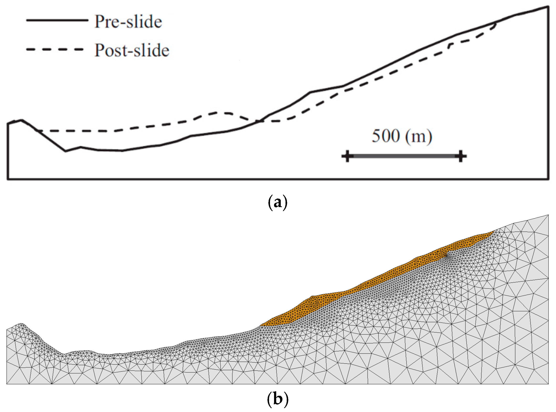
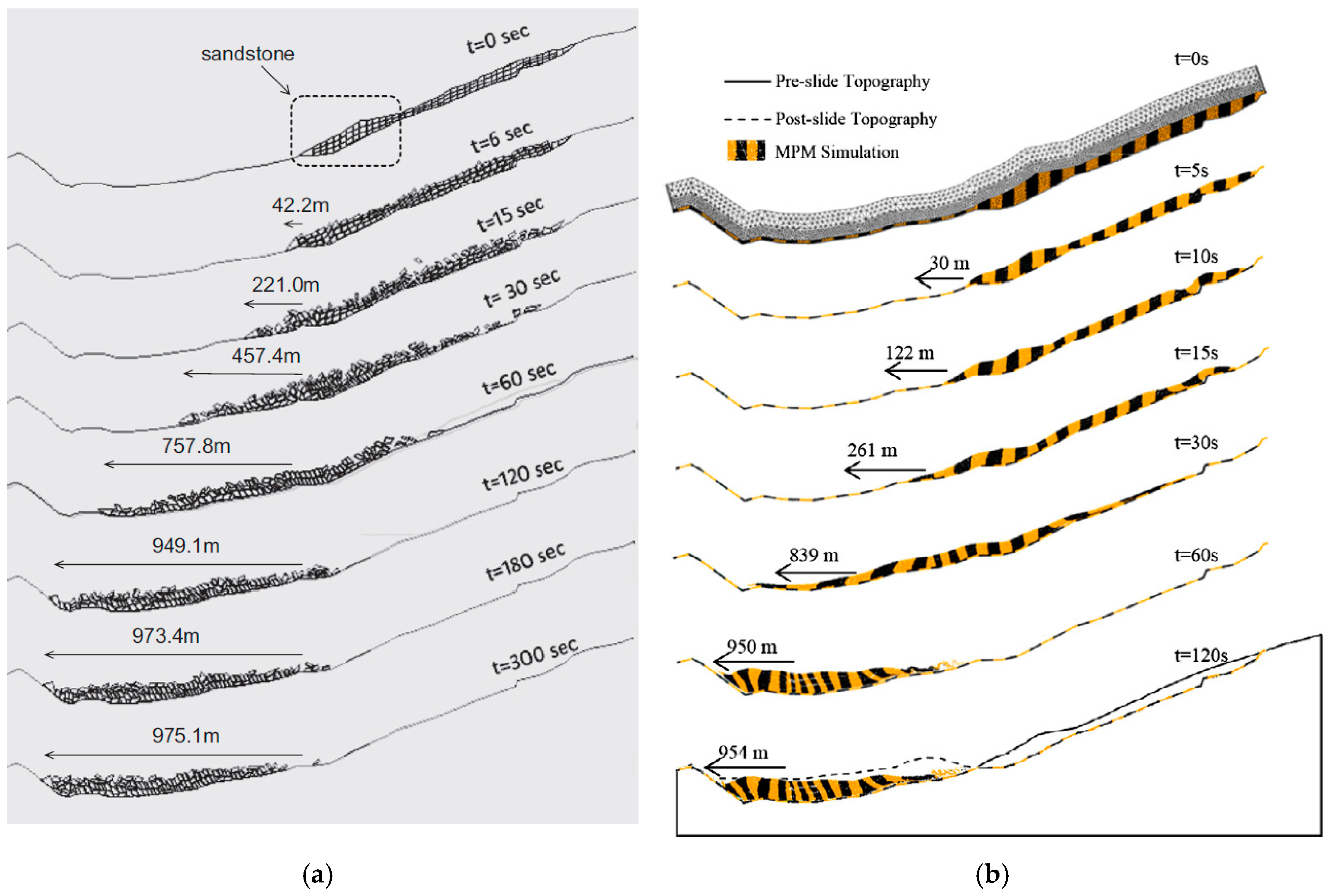
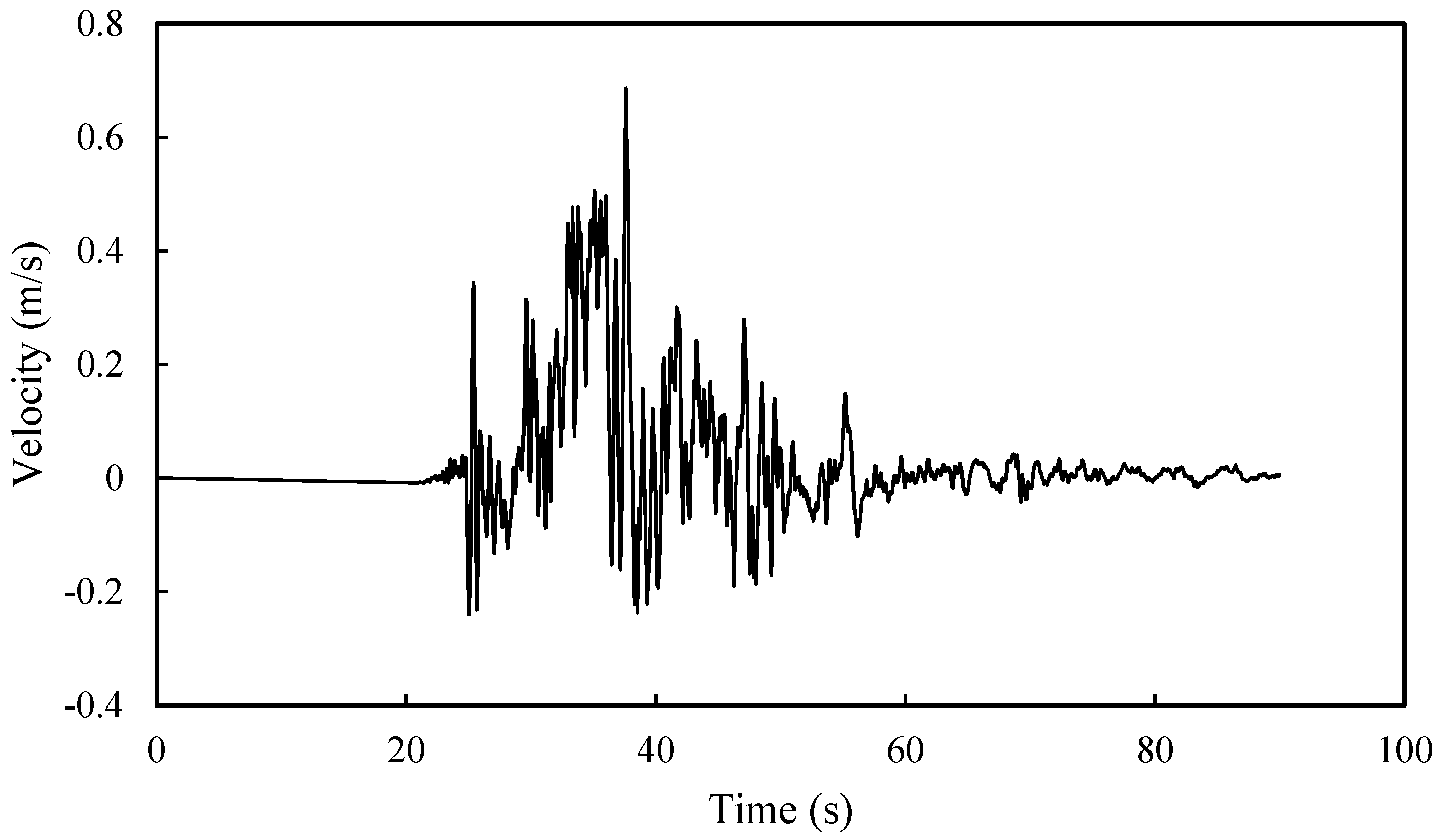
Configurations of landslide induced by the Chi-Chi earthquake are presented in Figure 6. The pre-and postslide configuration lines in Figure 6a are taken from reference [8] based on the site measurements where details can be found in Ref. [28]. In the FDEM modelling, 3072 elements are meshed in the mountain and 936 elements are meshed with rock blocks. The total computational time for this simulation is 119.1 h (up to t = 120 s). Fine mesh with the characteristic size of 10 m is employed for the slope surface of the mountain so that the shape of the slope surface is close to reality. On the other hand, coarse mesh with the characteristic size of 100 m is employed in the far field for the sake of computational efficiency. Rock blocks, with the characteristic size of 10 m, are modelled with individual noncohesive discrete elements. Horizontal ground motions recorded by the TCU072 station (see Figure 7) are used as the input earthquake excitation and applied to the mountain slope in the FDEM modelling. Material properties of rock blocks and the mountain are tabulated in

Table 3. Material properties of rock blocks and the mountain.

Young’s Modulus (GPa)	Poisson’s Ratio	Density (kg/m3)	Friction Angle (°)
7.57	0.19	2550	24

. Time step for this problem is 5 μs.

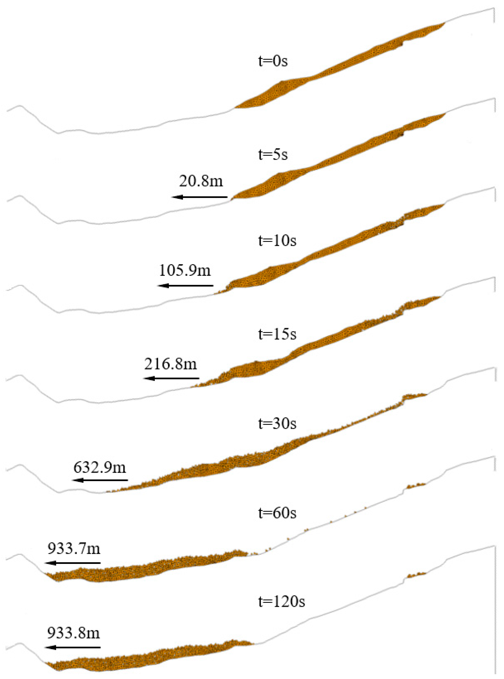
Figure 8 shows the progression of mass flow resulting from the landslide induced by ground excitations. The horizontal travelling distance of the front of the sliding mass is marked. It can be observed from Figure 8 that the sliding mass reaches the equilibrium around t = 120 s. Triggered by ground motions, the initially disintegrated rock blocks gradually slide to the foot of the mountain under gravity along the slope surface. The mass flow piles up at the foot of the mountain slope, resulting in a new slope surface which is in good agreement with the dash line in Figure 6a [8]. To better demonstrate the effectiveness of the FDEM in modelling this landslide process, results simulated by DEM [7] and MPM [8] are given in Figure 9 for comparison. It should be noted that the friction angle Φ = 22° in Figure 9a. This is because in reference [7], only data with Φ = 22° is available when cohesion c = 0.

The conclusion can be reached that the FDEM simulation agrees well with results from the DEM and MPM. For the travelling distance of front mass, results from the FDEM and DEM are in good agreement. For the slope process, the FDEM results are closer to the MPM results (particularly at t = 15 s and 30 s when the mass flow is dispersed a long distance along the slope surface). Fine-meshed rock blocks make the flowing mass more like granular material and thus results are closer to the MPM simulation.

It is also worth mentioning that although the FDEM results agree well with those from the DEM and MPM in general, there are still differences (e.g., the travelling distance of front mass). Furthermore, for the FDEM modelling, some rock blocks are still on the slope surface and have not fallen, and this phenomenon is not available in both DEM and MPM simulations. However, these differences are minor and can be considered acceptable due to the different methods employed.

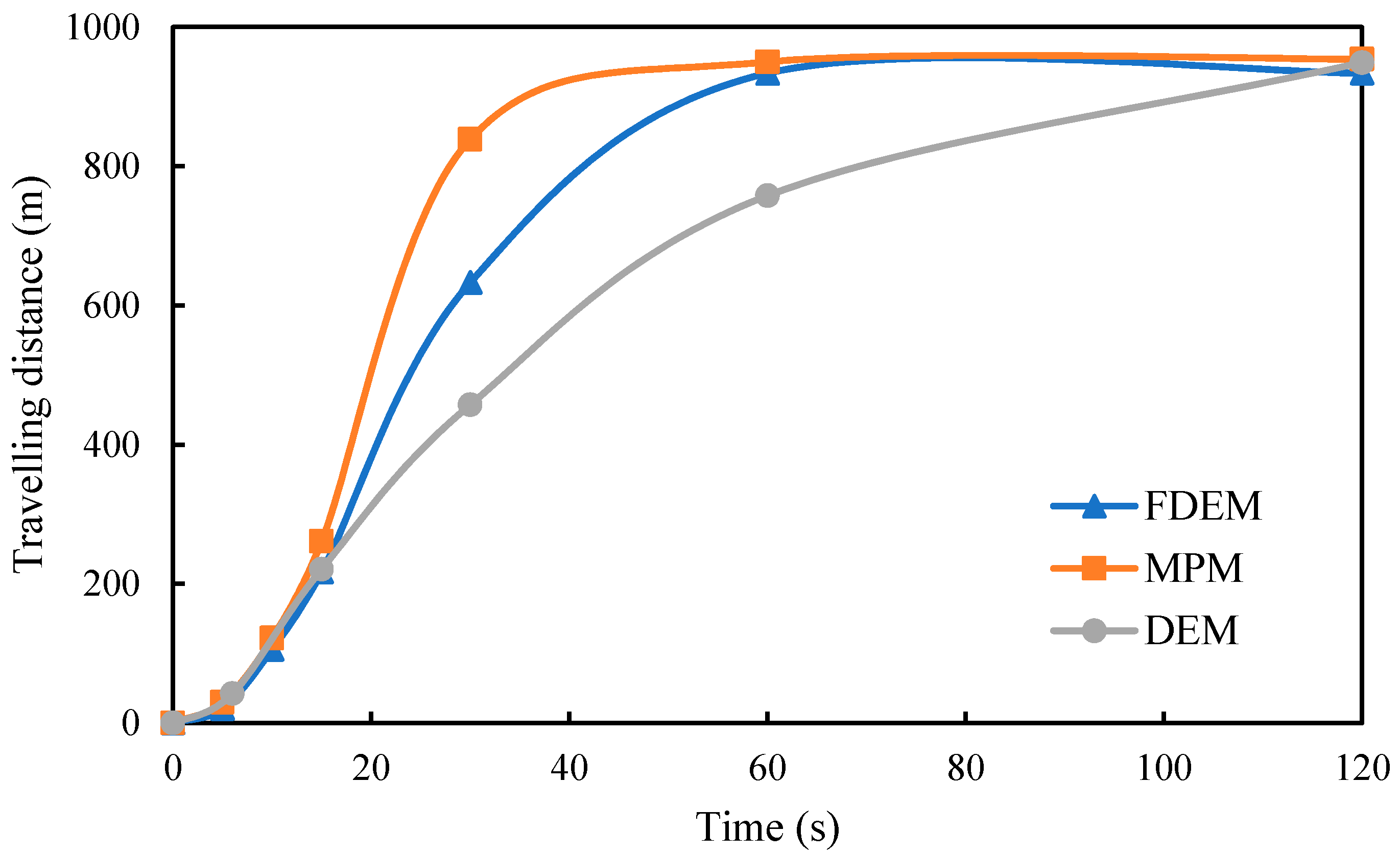
Figure 10 plots the horizontal travelling distances of the landslide simulated by the FDEM, DEM and MPM. It can be observed that all three curves agree quite well for 0 s ≤ t < 20 s. Then, major differences appear during 20 s ≤ t < 60 s, in which the result from the FDEM is between those from the DEM and MPM. Results from the FDEM and MPM converge around t = 60 s, which is much quicker than that from the DEM. Finally, all three curves converge consistently at t = 120 s.

Define the percentage differences η₁ and η₂ on the travelling distances between different methods as:

η₁ = (|Ω_FDEM-Ω_DEM|/Ω_FDEM) × 100%

(8)

η₂ = (|Ω_FDEM-Ω_MPM|/Ω_FDEM) × 100%

(9)

where Ω_FDEM, Ω_DEM and Ω_MPM are results from the FDEM, DEM and MPM, respectively.

Table 4. Differences on the travelling distances between different methods.

Time (s)	η1 (%)	η2 (%)
5	-	44.23
10	-	15.20
15	1.94	20.39
30	27.73	32.56
60	18.84	1.75
120	1.64	2.16

presents the percentage differences on the travelling distances between different methods.

From Table 4, the percentage difference between the FDEM and MPM is quite large at early stage although their travelling distance curves are very close as can be seen in Figure 10. Percentage differences of η₁ and η₂ are still quite noticeable between t = 30 s and t = 60 s. This is deemed as acceptable considering the different methods employed.

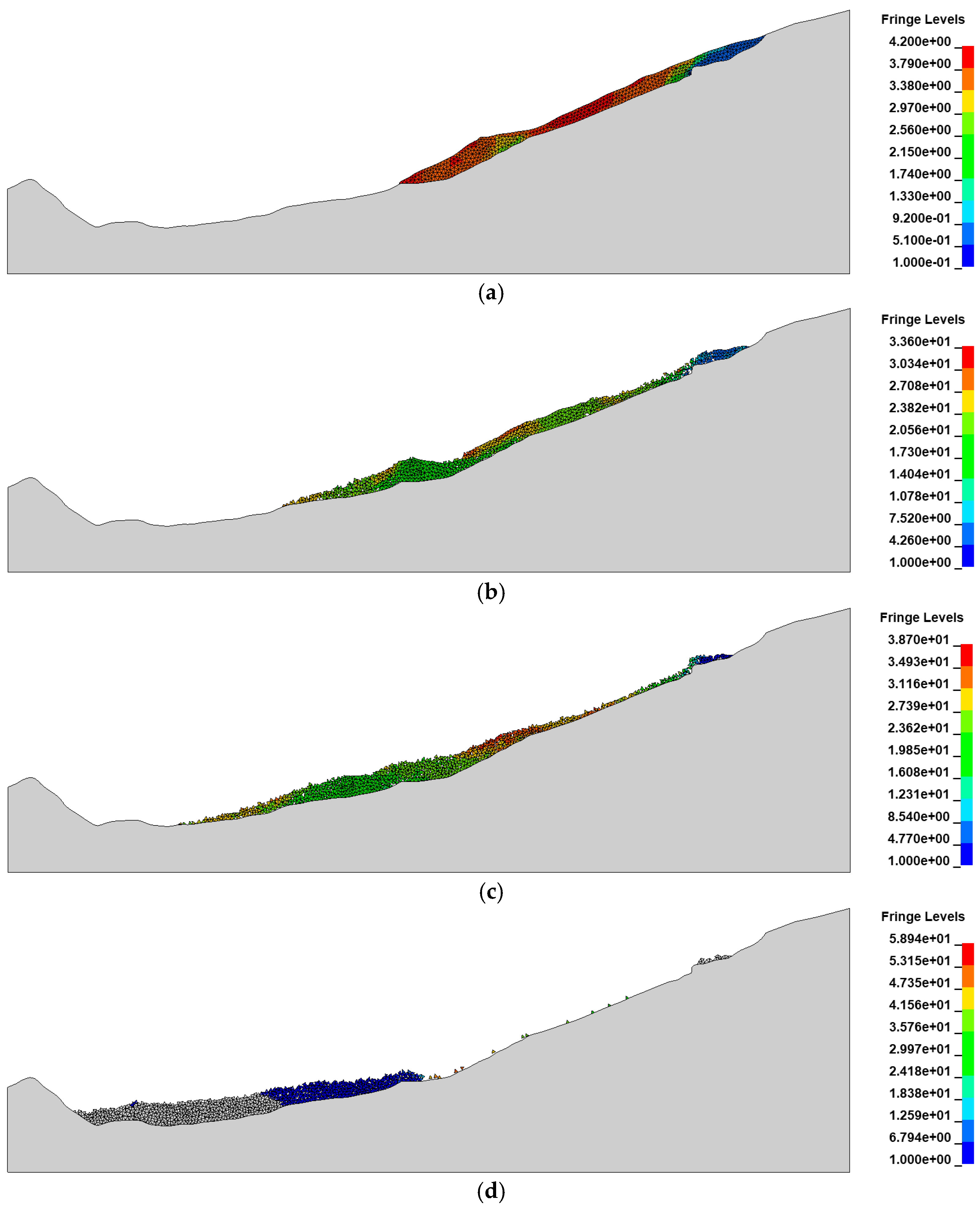
The velocity contour plotting of the landslide is given in Figure 11. It can be observed that initial velocity is passed to individual rock blocks with the motion of mountain (t = 2.5 s). The rock blocks slide gradually along the slope surface, and the toe and tail parts have higher velocities over other parts (see Figure 11b,c). When these blocks are accumulated in the lower basin of the mountain, the velocities almost drop to zero at around t = 60 s. It is worth mentioning that compared with the velocities and movements of individual rock blocks, the motion of the mountain is quite small. This suggests that for unstable mountainous areas, small base motions may result in disastrous landslide consequences.

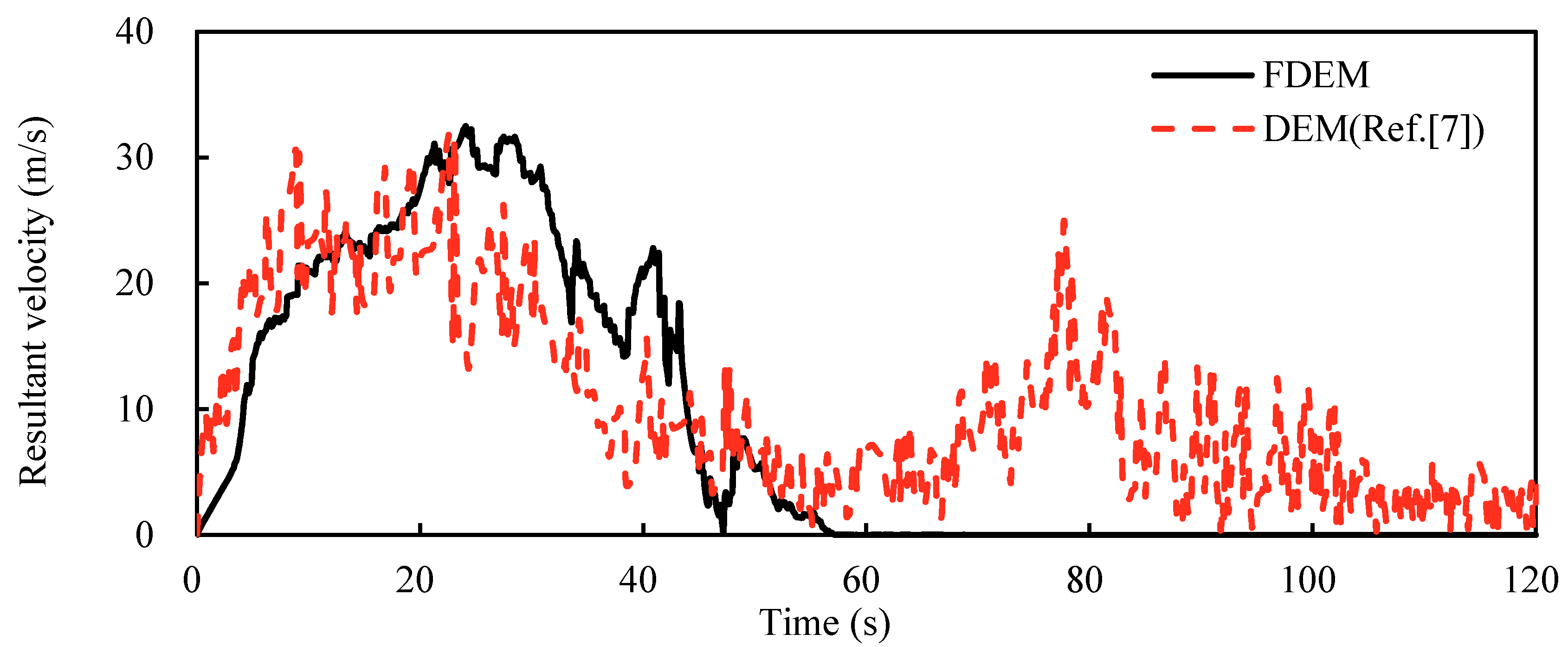
Figure 12 shows the resultant velocity of the toe block. For FDEM modelling, it can be observed that the velocity increases and reaches its peak between t = 20 s and 30 s. Afterwards, the velocity decreases dramatically and actually there is no residual velocity any longer after t = 60 s. This behaviour is in good agreement with DEM results from reference [7] before t = 60 s. In the DEM simulation, the velocity is still oscillating up to t = 120 s and reaches a second peak around t = 80 s, which is not realistic as the toe block has rested. The oscillation behaviour is not observed in the FDEM simulation, demonstrating that the FDEM modelling is more realistic and has advantages over the DEM modelling on velocity convergence.

5. Concluding Remarks

In this paper, the slope failure behaviour of noncohesive media under gravity and earthquake excitation is investigated using the two-dimensional combined finite–discrete element method (FDEM). Basic aspects of the FDEM are addressed, and two examples are presented for comparison and validation.

In example I, gravity is applied to a rectangular noncohesive soil heap. The soil heap is half bounded by a steel frame and consequently, the free vertical surface will fail naturally under gravity. The FDEM results are compared with data from SPH simulation, and good agreement is reached. Failure mode, repose angle and slope distance from the FDEM modelling agree quite well with those from SPH simulation.

In example II, the Chiu-fen-erh-shan landslide induced by the Chi-Chi earthquake is studied using the FDEM. Noncohesive rock blocks are defined and the mountain is subjected to ground excitations. In the FDEM modelling, the mass flow of rock blocks is formed and the movement along the slope surface is recorded. By comparing the failure mode and horizontal travelling distance of the toe block with those from the DEM and MPM, it can be concluded that good agreement is reached. The FDEM is capable of simulating landslide behaviour of noncohesive rock blocks under earthquake.

It should be noted that there are some differences between the results from the FDEM and results from existing literature in both examples. A clear sliding surface is observed in FDEM simulation in example I, while it is not available in SPH simulation, suggesting that the capability of particle movement in SPH simulation is larger. In example II, the finally formed slope surface by the FDEM is closer to the on-site record. These characteristics are rooted in the natural merits of the FDEM, showing that the FDEM has advantages over other computational tools in modelling slope failure behaviour of noncohesive media under both static and dynamic loads.

Although this paper is based on 2D and may have some limitations for extending obtained results to 3D, it provides a new insight into the slope failure behaviour of noncohesive media using a novel computational approach, that is, the FDEM. By validation, the FDEM is proven to be applicable and reliable in modelling the slope failure of noncohesive media under both gravity and ground motions. Relevant three-dimensional modelling is under development and will be discussed in another article.