Convergence Optimization and Verification for Single-Channel Remote Parameter Control of a Nonlinear System

Featured Application

The work of this paper may be applied to road simulation test, fatigue vibration test and other experimental tests, for the automobile and its parts or other vibration test occasions such as building or bridge model vibration test.

Abstract

In this paper, the theory of RPC (remote parameter control) iteration process of linear situation without and with iteration coefficient as well as nonlinear situation with coefficient is analyzed. The influence of iteration coefficient on iterative convergence control condition is analyzed. Two kinds of optimized control method for iteration coefficient based on the system transfer function estimation are proposed. A lightweight motorcycle and electro-hydraulic servo road vibration test bench are used to verify the feasibility of the optimized control methods for the reproduction of road profiles of SISO (single-input, single-output) system. According to the experiment result, which is the RMS (root mean square) of the NSRE (normalized spectrum of response error) of system, the convergent precision, convergent speed and iteration stability are discussed to present the advantage and disadvantage of the optimized control methods. Compared with three commonly used manual methods, the result shows the rapidity and stability of optimized control methods.

1. Introduction

Different from direct quantitative determination of speed or torque, the road fluctuation is a kind of random vibration signal, which is difficult to collect [1]. As such, so the sinusoidal frequency signal is mainly used as input in an early-stage vibration experiment system [2]. After the experimental method of random signal power spectrum regeneration was invented by Edwin A. Sloane in the 1970s [2], the random vibration experiment platform for road simulation is developed gradually.

The ultimate goal of remote parameter control (RPC) is to achieve the desired response of the SUT (system under test) in the real environment and reproduce the desired response in the laboratory environment, so that the SUT in the laboratory can achieve the same experimental effect as in the real environment. Therefore, the cost of experimental verification and the time of verification is reduced, as well as the experimental environment could be controlled [1,2,3]. In most cases, when the SUT is tested in a real environment, only response—but no input—can be obtained, and the response characteristics between the output and input of the SUT are also unknown. The RPC could obtain the desired output of the SUT by controlling the input of the SUT through transfer function (TF) estimation and iterative control.

The most successful commercial applications of the reproduction system for the random vibration are RPC launched by MTS Corp. in 1977 [3], and TWR (time waveform replication) of LMS Corp. [4,5], in which TWR is nowadays mainly used in MAST (multi-axial simulation table), thus RPC is not only used in MAST but also used in a RTS (road test simulator) [6]. There are other applications of road reproduction experiment as well, including ITFC (Iterative Transfer Function Compensation) launched by Schehck Corp. in 1979, and IDC (Iterative Deconvolution Control) launched by Faithurst Corp. in 1987. Their basic principle of iteration is more or less the same, which is RPC iterative control algorithm [7,8].

The RPC algorithm mostly used in RTS is a kind of iteration algorithm based on a linear approximation system. Therefore in practical application, if the system is highly nonlinear, the iteration coefficient for correction needs special attention, otherwise the iteration may be easy to diverge [9,10].

The most recent research on RPC algorithm are described herein: Multichannel decoupling used for multi-input iterative system control [11]; Combining multichannel electro-hydraulic servo online control with RPC offline iteration [12]; Using different frequency response characteristic estimation methods to obtain the estimation of frequency response function [13]; Proposing the method of value of drive correction coefficient based on the results to reduce the artificial participation and optimize the iterative robustness [8]; To optimize the iterative process by filtering the drive correction [9]; Proposing the method of updating the TF based on the system characteristics [14] and the method of system nonlinear and linear partial separation and identification [15] to improve the convergence of the system; Proposing the method of system linear partial experiment identification, nonlinear partial SVM (support vector machine) identification to obtain the accurate system transfer function [16]; Application on the parallel vibration table of various degrees of freedom [17,18] and extending the application range to other vibration areas like a seismic simulation [6].

At present, most of the studies of RPC algorithm have made some progress on theoretical analysis like global convergence theory analysis, the theoretical basis of the correction coefficient applied to nonlinear system, and the relationship between frequency response characteristics of test system and frequency response bandwidth of the whole iterative process [8].

As for references, previous work has done a lot of researches and contributions to the RPC theory, but most of previous work only made literatures and process descriptions of the RPC process, without detailed theoretical descriptions and without discussing the convergence of the nonlinear system.

In this paper, by summarizing the previous work, a relatively detailed theoretical description of the RPC process is made, and the convergence condition of the nonlinear system is discussed. On this basis, a calculation method of the iteration coefficient is proposed and verified.

This paper focuses on theory analysis of RPC iteration process of linear and nonlinear conditions. The theory analysis of linear condition is previous work, while the theory analysis of nonlinear condition is the work of this paper. The effect of iteration coefficient of the drive correction on accuracy, rapidity and stability in the iteration process is discussed, and two kinds of optimized control method for iteration coefficient based on the system transfer function estimation on each step of iteration are proposed.

To test the adaptability and stability of the method, three kinds of manual methods based on engineering experience are used to compare with the optimized methods. These methods are tested on the front half part of a motorbike, driven by electro-hydraulic vertical road vibration test bench and responded by IEPE (integrated electronics piezoelectric) accelerometer. The pros and cons of optimized methods and manual methods are discussed in different conditions like the convergent precision, convergent speed and iteration stability.

2. Principle

2.1. RPC Theory

The RPC was proposed by Dr. Richard A. Lund of MTS Systems Corp. in 1970s, which is a theory and technology of random environment simulation test [19]. Compared with the early-stage regular wave simulation test, the RPC is closer to the real operation condition.

RPC is a closed-loop iterative control method, which takes the difference between the desired response and the current iteration response (response error) as feedback, to obtain the input compensation value (drive correction) through the controller composed with linear TF estimation and iteration coefficient, and then carries out the next iteration. The RPC uses the calculated system inputs, through the system TF, to control the system outputs far away from the inputs, so it is called remote parameter control.

The word “far away” or “remote” in RPC means that the control quantity (input) and the controlled quantity (output) are far away from each other. For example, the control quantity in this paper is the displacement of the actuator of the test bench, and the controlled quantity is the acceleration on the vehicle frame. At the same time, RPC aims to reproduce the desired response of the SUT in the laboratory environment, while the desired response is achieved in the real environment. The laboratory environment and the real environment are also geographically far away from each other.

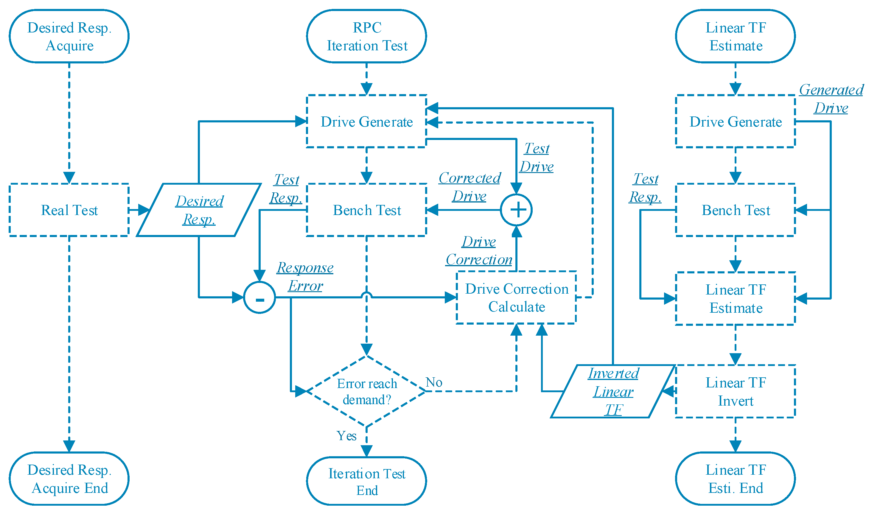
The purpose of RPC is to calculate the input signal with the system characteristics and to get the desired responses by using random function theory. The RPC mainly contains three parts: the desired response acquirement, the linear TF estimation and the iteration test [20,21], as shown in Figure 1:

The drive of the Real Test (on a real road) and TF of SUT under the Real Test are unknown, and other signals including response of SUT under the Real Test (desired response), Generated Drive in Linear TF Estimate (standard road) and response of bench test are known. In this paper, the real road is already obtained, but it is just a precondition.

The real road is taken as input and the experiment was carried out on the test bench to simulate the experiment process on the real road. The response obtained is taken as the Desired Response and used as the initial condition to verify the control algorithm of this paper, for example, the data acquired by the transducers on the vehicle which runs on the real road.

The linear TF estimation is obtained by vector division with the Fourier transform of generated drive (standard road) and test response. The standard road is usually generated based on standard condition that close to real road or experience. The inverse linear TF is obtained by taking the reciprocal of the linear TF estimation.

The iteration coefficient is contained in the drive correction calculation. For RPC, the displacement of the actuator of the test bench is controlled, and it is the corrected drive obtained by adding the previous drive and the drive correction. The iteration test is continuously generating drive and doing bench test until the error between desired response and test response reaches the demand. Otherwise, the response error is used to calculate the drive correction for the new drive, then test process iterates. The detail of calculation will be described later.

The bench test means that the SUT is test on the test bench in the experiment lab, while the real test means that the SUT is test on the real road. The outputs of bench test and real test should be the same, because the goal of RPC is to reproduce the desired response of the SUT on the test bench and the desired response is the output of the SUT in real test. We change the iteration coefficient to adjust the “size” of drive correction to control the input of iteration so as to make the iterative process more accurate, fast and stable.

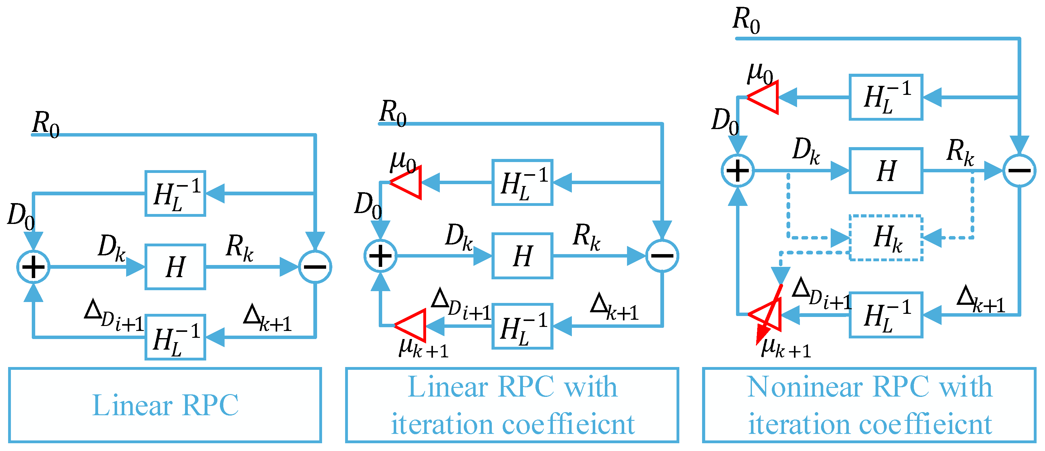
The experimental theory of RPC and the iterative process of linear system are all the work of predecessors. In this paper, the unified elaboration and convergence analysis of linear RPC is carried out. The iterative process of nonlinear system and its convergence analysis in the last section are studied in this paper, which improves the traditional linear RPC theory.

In this paper, three types of RPC iterative processes are discussed, including linear systems without iterative coefficients, linear systems with iterative parameters, and nonlinear systems with iterative parameters. As shown in Figure 2.

In the following sections, the specific iterative process is theoretically derived and the iterative convergence conditions are discussed.

2.2. Linear Situation

Firstly, the simplest condition of RPC process, the linear situation should be discussed. The expression of linear system is shown below:

$$r=h\left(d\right)\stackrel{Fouriertransform}{\Rightarrow }R=HD$$

(1)

where the $d$,$r$ are the time series of drive signals and response signals of the system, $h( )$ is the system TF in time domain, equivalently, the $R$, $D$ are the Fourier transform of drives and responses, $H$ is the system TF in frequency domain.

It assumes that the system is linear and invertible, error and noise are not considered. $R_0$ is the desired response,$D_0$ is the initial drive, ${\Delta }_i$ is the ith response error, ${\Delta }_D{}_i$ is ith drive correction, $D_i$ is the drive after $i$ times of correction, $H_L^{-1}$ is the inverse linear TF. The linear TF estimation of the system is expressed below:

$$H_L=R_s/D_s$$

(2)

where the $D_s$ is the Fourier transform of standard road and the $R_s$ is the response of SUT while the drive is $D_s$.

$H{H}_L^{-1}$ is set as $P$ which represents TF deviation ratio. Then the initial drive is:

$$D_0=H_L^{-1}{R}_0$$

(3)

The first response error is:

$${\Delta }_1=R_0-H{D}_0=\left(I-P\right)R_0$$

(4)

The first drive correction is:

$${\Delta }_D{}_1=H_L^{-1}{\Delta }_1=H_L^{-1}\left(I-P\right)R_0$$

(5)

The first drive is

$$D_1=D_0+{\Delta }_D{}_1$$

(6)

The first drive is the sum of initial drive and first drive correction. When $k\ge 1$, the response error, drive correction and drive after k times iteration are:

$${\Delta }_k=R_0-H{D}_{k-1}=\left(I-P\right){\Delta }_{k-1}$$

(7)

$${\Delta }_D{}_k=H_L^{-1}{\Delta }_k$$

(8)

$$D_k=D_{k-1}+{\Delta }_D{}_k$$

(9)

The kth drive is the sum of k−1th drive and kth drive correction. So the expressions of ith drive correction and drive after k times of correction are:

$${\Delta }_D{}_i=H_L^{-1}{\left(I-P\right)}^i{R}_0,i\ge 1$$

(10)

$$D_k=D_0+{\displaystyle \sum }_{i=1}^k{\Delta }_D{}_i$$

(11)

In the linear situation, the drive correction is geometric progression, so the kth drive is the sum of the geometric progression. For real number, if the ratio of the geometric progression is less than 1, the progression converges. For the complex number, the convergence condition is that the magnitude of the ratio less than 1. And for the complex number vector which is the situation in this paper, then the convergence condition is that the magnitude of the complex vector of the response error ratio $\left(I-P\right)$ is less than 1.

The convergence condition is expressed as $\left|I-P\right|<I$. If the convergence condition satisfies, then infth drive correction trends to zero.

$$\underset{i\to \infty }{\lim }{\Delta }_D{}_i=0$$

(12)

The series of the drive converges, then the drive after infinite steps is:

$$D_{\infty }=D_0+{\displaystyle \sum }_{i=1}^{\infty }{\Delta }_D{}_i=H_L^{-1}\left({\displaystyle \sum }_{i=0}^{\infty }{\left(I-P\right)}^i\right)R_0=H_L^{-1}{P}^{-1}{R}_0=H^{-1}{R}_0$$

(13)

The actual drive for the desired response is:

$$D_R=H^{-1}{R}_0$$

(14)

The result after infinite times of iteration shows that the reproduced drive and response meet the desired drive and response.

2.3. Linear Situation with Coefficient

With the change of experimental condition, the TF deviation ratio may not satisfy the above convergence condition $\left|I-P\right|<I$. If so, the iteration diverges, which should be solved.

For a linear system, this is mainly caused by the estimation error between the linear TF $H_L$ and the actual TF $H$, especially when the noise of data acquisition is great. For most inertial systems, the abnormal high frequency response caused by noise may override the relatively small response characteristics of the system itself in the high frequency part.

Normally. the drive correction is scaled by a factor called iteration coefficient which is represented by $\mu$ in this paper. The ${\mu }_k$ represents a series of constants used in each iteration step.

Thus, the initial conditions are changed. The initial drive, the first response error and first drive correction are:

$$D_0={\mu }_0{H}_L^{-1}{R}_0$$

(15)

$${\Delta }_1=R_0-H{D}_0=\left(I-{\mu }_{0}P\right)R_0$$

(16)

$${\Delta }_D{}_1=H_L^{-1}{\Delta }_1=H_L^{-1}\left(I-{\mu }_{0}P\right)R_0$$

(17)

The response error after k times of iteration is:

$${\Delta }_k=R_0-H{D}_{k-1}=\left(I-{\mu }_{k-1}P\right){\Delta }_{k-1}$$

(18)

The drive after k times correction is:

$$D_k=D_{k-1}+{\mu }_k{\Delta }_D{}_k$$

(19)

The ith drive correction and the drive after k times correction are:

$${\Delta }_D{}_i=H_L^{-1}\left[{\displaystyle \prod }_{m=0}^{i-1}\left(I-{\mu }_{m}P\right)\right]R_0,i\ge 1$$

(20)

$$D_k=D_0+{\displaystyle \sum }_{i=1}^k{\mu }_i{\Delta }_D{}_i$$

(21)

In the case of a linear system, P stays the same. But in practice, the system is always non-linear, and the difference is the degree of non-linear. When the system is less nonlinear, P is close to I, so the convergence condition $\left|I-{\mu }_{i}P\right|<I$ can be satisfied when ${\mu }_i$ is close to 1.

According to engineering experience, the iteration coefficient is chosen to be $0\le {\mu }_i\le 1$. At the beginning of the iteration, because the drive and response of the iteration differ greatly from the desired value, so the drive correction will be large. Therefore, the selection of the iteration coefficient is small to avoid driving overshoot.

As a controlling method, if the TF deviation ratio without iteration coefficient is out of the convergence condition ($\left|I-P\right|\ge I$), then iteration coefficient is used to make the convergence condition satisfy ($\left|I-{\mu }_{i}P\right|<I$). If the convergence condition is achieved, the drive correction will trend to zero based on the expression of drive correction in equation (20).

$$\underset{i\to \infty }{\lim }{\Delta }_D{}_i=0$$

(22)

Based on the expression of drive and drive correction in equations (20) and (21), the last drive after infinite steps is

$$D_{\infty }\triangleq H_L^{-1}{S}_{\infty }{R}_0$$

(23)

where $S_{\infty }$ stands for composite gain and is expressed as:

$$S_{\infty }={\mu }_0+{\displaystyle \sum }_{i=1}^{\infty }{\mu }_i\left[{\displaystyle \prod }_{m=0}^{i-1}\left(I-{\mu }_{m}P\right)\right]$$

(24)

It is easy to approve that

$$1-P{S}_{\infty }={\displaystyle \prod }_{i=0}^{\infty }\left(I-{\mu }_{i}P\right)$$

(25)

If the convergence condition satisfies, then

$$1-P{S}_{\infty }=0$$

(26)

The composite gain is the inverse of the TF deviation ratio $P$:

$$S_{\infty }=P^{-1}$$

(27)

Finally, it can be proved that the last drive after infinite steps will be equal to the road drive:

$$D_{\infty }=H_L^{-1}{S}_{\infty }{R}_0=H_L^{-1}{P}^{-1}{R}_0=H^{-1}{R}_0$$

(28)

2.4. Nonlinear Situation

The previous experimental theory of RPC and the iterative process of linear system are the work of predecessors, and this paper has summarized and discussed. The following discussion of nonlinear RPC process and convergence condition is the work of this paper.

In most cases, the system is nonlinear, as shown in the definition below:

$$r=h\left(d\right)\stackrel{\mathrm{Fourier}\mathrm{transform}}{\Rightarrow }{R}_k=H\left(D_k\right)\stackrel{\mathrm{def}}{=}{H}_k{D}_k$$

(29)

where $H_k$ stands for the TF in frequency domain especially when the input is $D_k$. The system is nonlinear so the TF $H_k$ will change with the input, and the subscript of the TF represents the TF of the system at the kth input $D_k$.

It assumes that the correspondence between drive and TF $f.D_k⟼H_k$ is bijective.

As mentioned before, the TF deviation ratio may not satisfy the convergence conditions. But in nonlinear system, it is mostly caused by the nonlinear characteristics of system, which may cause the linear TF $H_L$ and the actual TF $H$ have great differences in the whole frequency range.

For the convenient, the k+1 times condition shows here instead of the k times before. The response error after k+1 times of iteration are:

$${\Delta }_{k+1}=R_0-H_k{D}_k\triangleq {\Psi }_k{\Delta }_k$$

(30)

where the error ratio ${\Psi }_k$ is:

$${\Psi }_k=\left[H_k{H}_{k-1}^{-1}-{\mu }_k\left(P_k+\frac{\partial H_k}{\partial D_k}{H}_L^{-1}{H}_{k-1}^{-1}{R}_0\right)\right]$$

(31)

where the TF deviation ratio $P_k=H_k{H}_L^{-1}$, and the $\partial H_k/\partial D_k$ represents the gradient of TF:

$$\frac{\partial H_k}{\partial D_k}\stackrel{\mathrm{def}}{=}\frac{H_k-H_{k-1}}{D_k-D_{k-1}},k\ge 1$$

(32)

While initial condition of the nonlinear system is the same as the scaled linear system as mentioned in Section 2.3, so the expression of the response error and drive correction after i times of iteration is:

$${\Delta }_D{}_{i+1}=H_L^{-1}{\Delta }_{i+1}, {\Delta }_{i+1}=\left({\displaystyle \prod }_{k=1}^i{\Psi }_k\right)\left(I-{\mu }_0{P}_0\right)R_0,i\ge 2$$

(33)

If the error ratio satisfies the convergence condition which is $\left|{\Psi }_k\right|<I$, the response error after infinite steps will trend to zero:

$$\underset{i\to \infty }{\lim }{\Delta }_{i+1}=0$$

(34)

Thus, the convergence condition of nonlinear system is different with linear system.

If the convergence condition is achieved, the response error after infinite steps will also tend to zero. Then based on the expression of response error in Equation (30), the response after infinite steps will be equal to the desired response:

$$\underset{i\to \infty }{\lim }{H}_i{D}_i=R_0=H_R{D}_R$$

(35)

If the correspondence between drive and TF $f.D_k⟼H_k$ is bijective, and with the assumption that $\partial H_k/\partial D_k$ is bounded, then when iteration drive trends to road drive $D_k⟶D_R$, the iteration TF will trend to road condition TF $H_k⟶H_R$.

Finally, the drive after infinite steps will tend to the road input:

$$\underset{i\to \infty }{\lim }{D}_i=D_R$$

(36)

3. Method

For an ideal linear system, the TF of the system does not change with the change of input, and external interference is ignored, then the iterative process naturally converges, so the participation of iterative parameters is not required. Since iterative parameters are not required, there is no need for iterative parameter calculation algorithm. But in reality, the ideal hardly exists. In modern vehicles, chassis, suspension and tires are almost always nonlinear systems. Experimental equipment cannot be perfect, so there will always be interference. Therefore, under realistic conditions, the iterative process always needs the participation of the iteration coefficient. The iterative method in this paper is to put forward the calculation strategy of the iterative coefficient according to the iterative convergence condition and apply the calculated iterative coefficient to the iterative process.

3.1. Control Strategy

The purpose of control is to make the series of drive converge with good stability and fast convergence rate.

The convergence condition is mentioned before, which makes the drive correction tend to zero:

$${\Delta }_D{}_k\to 0$$

(37)

For the nonlinear system in Equation (31), if the error ratio ${\Psi }_k$ is nearly zero:

$${\Psi }_k=H_k{H}_{k-1}^{-1}-{\mu }_k\left(P_k+\frac{\partial H_k}{\partial D_k}{H}_L^{-1}{H}_{k-1}^{-1}{R}_0\right)\to 0$$

(38)

Then the convergence will be fast and robust. The ${\Psi }_k$ could be divided into 2 parts, the TF ratio ${ℒ}_k$, and effective ratio ${ℳ}_k$:

$${ℒ}_k=H_k{H}_{k-1}^{-1}$$

(39)

$${ℳ}_k=P_k+\frac{\partial H_k}{\partial D_k}{H}_L^{-1}{H}_{k-1}^{-1}{R}_0$$

(40)

Then set ${\Psi }_k$ as 0, the ideal coefficient will be:

$${\mu }_k=\frac{{ℒ}_k}{{ℳ}_k}$$

(41)

While ${\mu }_k$ is numerical coefficient, and $H_k$ are complex sequence with frequency $f$ as independent variable, so ${\mu }_k$ is calculated as:

$$\frac{1}{{\mu }_k}=\Vert \frac{{ℳ}_k}{{ℒ}_k}\Vert =\Vert \frac{P_k+\frac{\partial H_k}{\partial D_k}{H}_L^{-1}{H}_{k-1}^{-1}{R}_0}{H_k{H}_{k-1}^{-1}}\Vert =\Vert P_{k-1}+\frac{\partial H_k}{\partial D_k}{H}_L^{-1}{H}_k^{-1}{R}_0\Vert$$

(42)

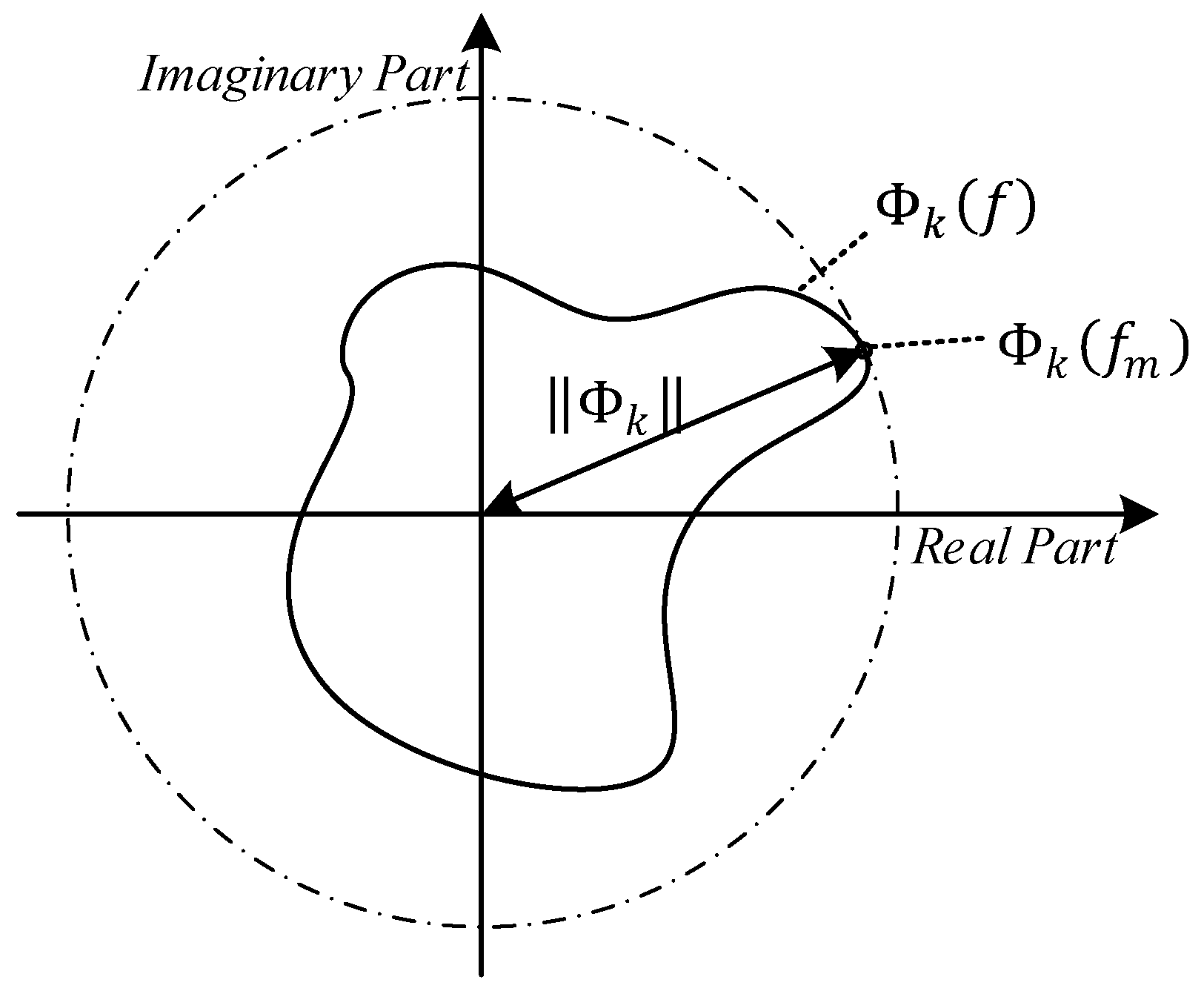
This iteration coefficient is calculated with vector norm to ensure stability, which makes the ${\mu }_k$ as small as possible. The vector norm ‖ ‖ is vector norm of complex sequence. The vector norm used here is the Maximum norm of the complex vector. For complex vector, first it takes the absolute value of complex numbers to get the real vector, and then takes the maximum norm of the real vector to get the maximum. The expression of the norm is shown as:

$$\Vert {\Phi }_k\Vert =max\left\{\left|{\Phi }_k\left(f\right)\right|\right\}=max\left\{\left|{\Phi }_k\left(f_1\right)\right|,\left|{\Phi }_k\left(f_2\right)\right|,\dots ,\left|{\Phi }_k\left(f_n\right)\right|\right\}$$

(43)

The vector norm is also shown in Figure 3:

As shown in Figure, the ${\Phi }_k$ is complex sequence with the frequency as the independent variable, and the complex point ${\Phi }_k\left(f_m\right)$ has the maximum magnitude, which is the value of the vector norm $\Vert {\Phi }_k\Vert$.

In short, the purpose of control strategy is to make the iterative process meet the convergence condition, as shown in Figure 4 below:

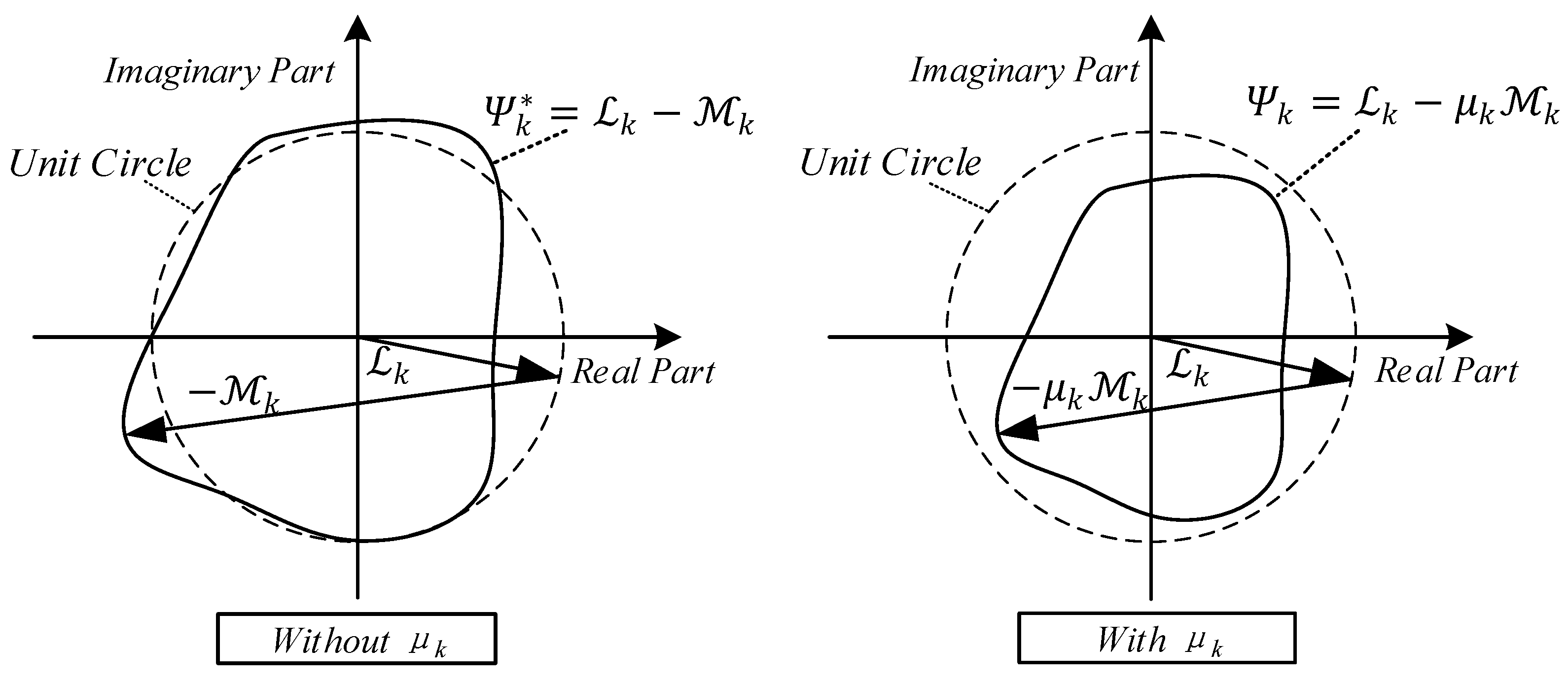
As shown in Figure 4, the error ratio ${\Psi }_k^{*}$ without iteration coefficient ${\mu }_k$ may be out of the Unit Circle, and the iteration coefficient ${\mu }_k$ can make the error ratio ${\Psi }_k$ be in the Unit Circle to meet the convergence condition and be as small as possible to make convergence fast. The Unit Circle is the complex circle with radius 1.

If the system is close to linear system, then the TF will basically remain unchanged, the TF ratio ${ℒ}_k$ will be close to 1 at the real axis. While the effective ratio ${ℳ}_k$ contains 2 parts, TF deviation ratio $P_k$ and the relative change amount of the TF. In addition, if the system is close to linear system, then the TF deviation ratio $P_k$ is close to 1, and the relative change amount of the TF is a small area around the original point.

3.2. Modified Strategy

Based on assumption of causality, $H_k$ can only be measured after $D_k$ has inputted into system, and $D_k=D_{k-1}+{\mu }_k{\Delta }_D{}_k$. Therefore, in the actual system, ${\mu }_k$ cannot be calculated from $H_k$, so the iteration coefficient has to be calculated by the results of the previous step.

$$\frac{1}{{\mu }_k}\cong \Vert P_{k-2}+\frac{\partial H_{k-1}}{\partial D_{k-1}}{H}_L^{-1}{H}_{k-1}^{-1}{R}_0\Vert ,k\ge 2$$

(44)

Then the initial and first correction values of iteration coefficient are:

$$\frac{1}{{\mu }_1}=\Vert P_0\Vert \hspace{1em}, \frac{1}{{\mu }_0}=k_0$$

(45)

The initial value ${\mu }_0$ can only be set manually, which usually takes a mid-value 0.5.

3.3. Simplified Strategy

In Section 3.1 and Section 3.2, the control strategy is discussed, but the computational capacity is large. Especially the TF gradient $\partial H_k/\partial D_k$ needs two times of TF $H_k$ and drive $D_k$, which also will use lots of memory.

When the whole system is a linear system, the TF will not change when the input drive signal changes, so the TF gradient will be always zero. When the system is approximately linear, the TF will change very little when the input drive signal changes, so the TF gradient will be approximately zero. Therefore, when the system is close to linear, the calculation could be simplified by ignoring the TF gradient. And if the TF gradient is small enough to ignore, the strategy based on (42) could be simplified as below:

$$\frac{1}{{\mu }_k}\approx \Vert P_{k-1}\Vert ,k\ge 1$$

(46)

3.4. Iteration Filter

The operating frequency and sampling frequency of the system are 1 kHz, so based on Nyquist sampling theorem, the effective spectrum bandwidth is 500 Hz. But in actual situation, excessive frequency bandwidth is meaningless, so the maximum frequency in this paper is set as 200 Hz. At the same time, due to the limitation of the driving stroke of the system, and the sensor's low frequency response is very poor, the minimum frequency in this paper is set as 0.2 Hz.

In this paper, the filter is a simple first-order Butterworth high-pass filter with cutoff frequency at 0.2 Hz, and a first-order Butterworth low-pass filter with cutoff frequency at 200Hz. The filter is applied on the drive correction and in the calculation process of the iteration coefficient.

3.5. Error Evaluation

The termination condition of iteration is the root mean squared (RMS) of the normalized spectrum of response error (NSRE), which is also a main evaluating standard for iteration convergence. The expression of NSRE is shown below:

$${\overline{\Delta }}_k=\frac{{\Delta }_k}{\mathrm{RMS}\left(\left|R_0\right|\right)}$$

(47)

where the RMS () is the root mean square function for the vector.

The expression of termination condition is the RMS of NSRE:

$${\mathrm{r}}_k=\mathrm{RMS}\left(\left|{\overline{\Delta }}_k\right|\right)$$

(48)

3.6. Road Spectral Transform

The frequency of road is space frequency n (with dimension m⁻¹), so the PSD (power spectral density) of road is space PSD (with dimension m²/m⁻¹). For experiment and data process, the space PSD need to be transformed into time PSD (with dimension m²/s⁻¹). The transform expression is:

$$f=vn,G_q\left(f\right)=G_q\left(n\right)/v$$

(49)

where $v$ is vehicle speed, $f$ is time frequency, $n$ is space frequency, $G_q\left(f\right)$ and $G_q\left(n\right)$ are PSD in time and in space.

According to the definition of PSD, the PSD of space and time frequency can be expressed as $G_q\left(n\right)=\underset{\Delta n\to 0}{\lim }\frac{{\sigma }_{q~\Delta n}^2}{\Delta n},G_q\left(f\right)=\underset{\Delta f\to 0}{\lim }\frac{{\sigma }_{q~\Delta f}^2}{\Delta f}$, where ${\sigma }_{q~\Delta n}^2$ is the power in the frequency range $\Delta n$ and ${\sigma }_{q~\Delta f}^2$ is the power in the frequency range $\Delta f$. In the case of vehicle speed $v$, the harmonic component of the vertical irregularity displacement $q$ contained in the space frequency band is the same as that in the time frequency band, so the power is also the same. According to the relation between space frequency and time frequency $f=vn$, the relation between space frequency band and time frequency band can be known $\Delta f=v\Delta n$, so the conversion relation between space PSD and time PSD is $G_q\left(f\right)=G_q\left(n\right)/v$.

4. Experiment Preparation

4.1. Experiment Environment

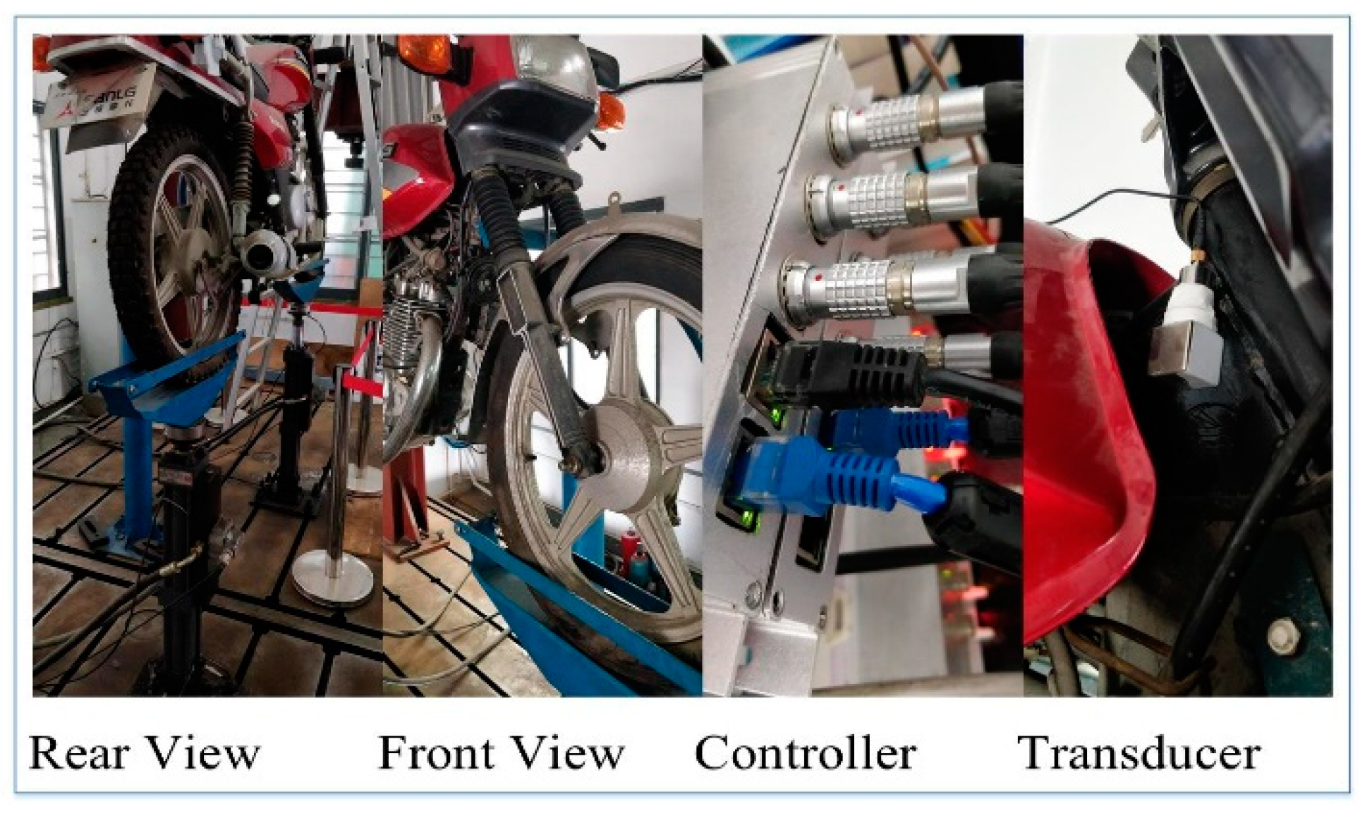
As shown in Figure 5 and Figure 6, the test bench is an electro-hydraulic servo actuator embedded with LVDT (linear variable differential transformer) displacement transducer and piezoelectric load sensor. The actuator is controlled by filed bus based real time feedback controller. The system under test is the front half of a motorbike, because only single channel is discussed in this paper. The transducer is the IEPE (integrated electronics piezoelectric) accelerometer, which fixed to the frame with neodymium magnet.

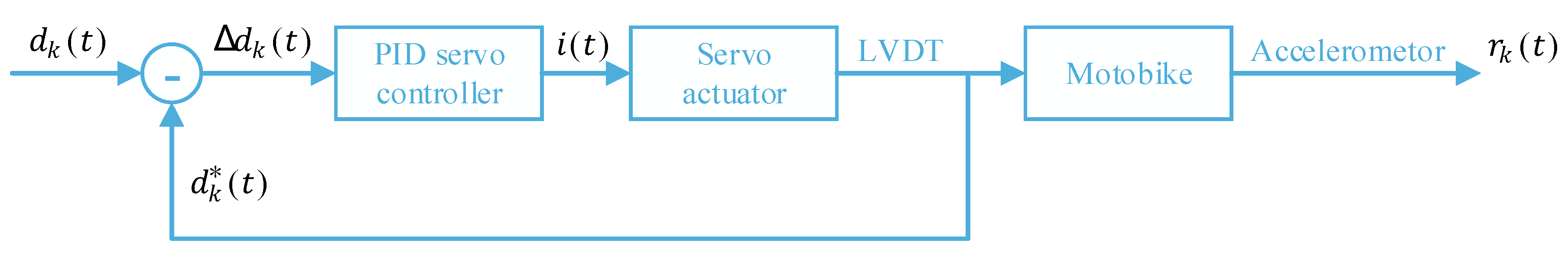
The servo feedback control method of the controller is frequently-used PID control without adaptive algorithms. The PID parameter is separately 0.75, 0.05 and 0.0005. For the test equipment, the control object is the electro-hydraulic servo actuator. PID servo controller controls the servo valve to drive the hydraulic cylinder movement, so that the piston displacement of the hydraulic cylinder is consistent with the drive signal of RPC, as the input signal of the system. The $d_k\left(t\right)$ and $d_k^{*}\left(t\right)$ are the time-domain drive signal and the actuator displacement signal collected by the sensor. The difference between the driving signal and the feedback signal $\Delta d_k\left(t\right)$ is taken as the input of PID servo controller, and the controller output is the current signal $i\left(t\right)$. The current signal drives the servo actuator and the servo actuator drives the wheels of the motorcycle. The acceleration signal of the motorcycle body $r_k\left(t\right)$ is collected by the sensor and taken as the output of the system.

4.2. Experiment Parameters

The parameters of the experiment are listed in

Table 1. Experiment parameter list.

Name	Value	Dimension (Remark)
Experiment duration	199.68	s
Drive frequency	1000	Hz
Sampling frequency	1000	Hz
Servo valve type	Moog G761-3010B	(2 stage servo valve)
Hydraulic actuator type	R-ZD-0020-0200	(Symmetrical cylinder)
Accelerometer type	B&W Tech. 14100	(IEPE)
Motorbike type	Sanlg SL125-2E	(Lightweight motorbike)
Hydraulic oil Pressure	2.1	MPa
Transducer limit	±500	m/s2
Transducer accuracy	0.001	m/s2
Transducer bandwidth	0.2–10000	Hz
Motorbike tire pressure	150	kPa
Motorbike wheel base	1.350	m
Motorbike total mass	83.35	kg
Motorbike barycenter	0.732	m (Horizontal distance from front axle)
Front sensor location	0.351, 0.542	m (Horizontal, vertical distance from front axle)
Controller P parameter	0.75	A/m
Controller I parameter	0.05	A/(m*s)
Controller D parameter	0.0005	A*s/m
Control accuracy	0.02	mm
Gravity	9.794	m/s2

below:

4.3. Experimental Method

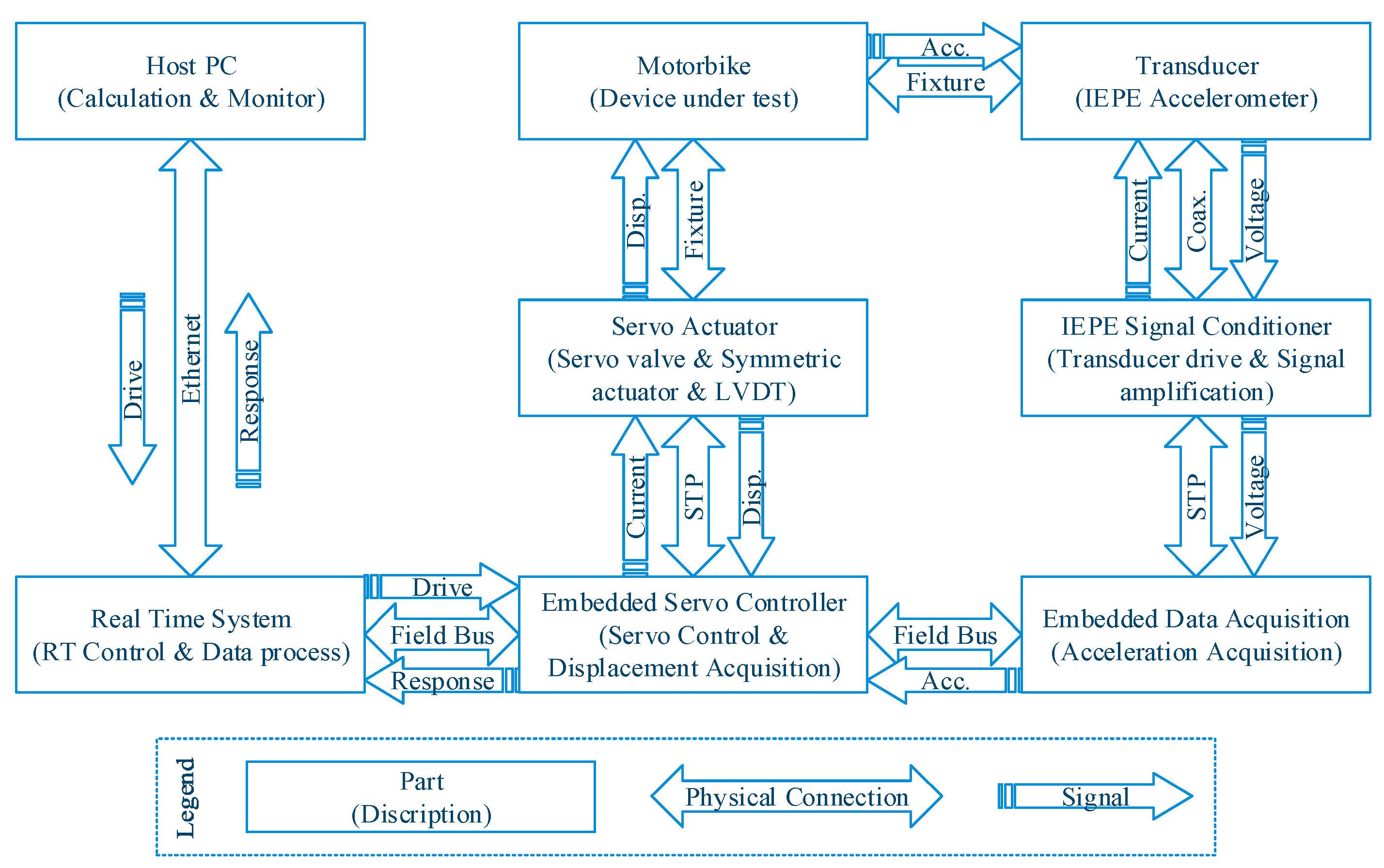
As shown in the Figure 7, the whole experiment system contains eight parts, including the host PC, real-time system, motorbike, servo actuator, embedded servo controller, transducer, IEPE signal conditioner and embedded data acquisition.

The host PC is used for iteration calculation and monitor, as well as sending drive data to real-time system and receiving response data from real-time system over the ethernet. The real-time system is used for real time control and data processing, as well as exchanging data with the host PC over ethernet as well as with the embedded servo controller and embedded data acquisition over the field bus.

The servo actuator contains a servo valve, symmetric actuator and LVDT used for displacement measurement. The controller and the servo actuator form the displacement closed loop, to make sure that the iterative displacement drive is accurately generated and applied to the wheel of the motorbike. The motorbike is the device under test and driven by the piston of the actuator.

The transducer is an IEPE accelerometer, mounted on the body of the motorbike by neodymium magnet, and used to measure the vertical acceleration of the motorbike as the response of the iteration. The IEPE signal conditioner is connected with the sensor by coaxial cable (coax. for short) to stimulate the sensor, to amplify and filter the signal collected, and then it transmits the adjusted analog signal to the data acquisition equipment over the STP (shield twisted pair). The embedded data acquisition is used to collect analog signal transmitted by signal conditioner and carry out A/D (analog to digital) conversion, and then transmits the digital response signal to the real-time system over the fieldbus.

The whole system is based on real-time control and synchronous sampling technology, so the time difference between control and sampling is less than 10 microseconds, which ensures the accuracy of experimental control and sampling phase. The control and sampling time difference of the experimental equipment has no relation with the natural frequency of the system. Because according to our experience, when the control and sampling time difference of experimental equipment changes greatly, for example, if it is greater than 1 millisecond in this experiment, and it fluctuates in each iteration, then the error of system TF estimation will occur due to the change of phase difference between input and output, so that the iteration may diverge. The time difference within 10 microseconds is satisfactory, and the interference caused by this factor is not needed to be considered in the whole iteration process.

4.4. Experiment Equipment TF

Because there are many components in the whole electro-hydraulic servo experimental system, including pump station, high-pressure pipeline, electro-hydraulic servo valve, hydraulic cylinder and closed-loop PID servo controller, and the parameters of many components are unknown. It is difficult to give a complete expression of the TF of the experimental system. Therefore, the closed-loop frequency domain response diagram of the servo system is added in this section.

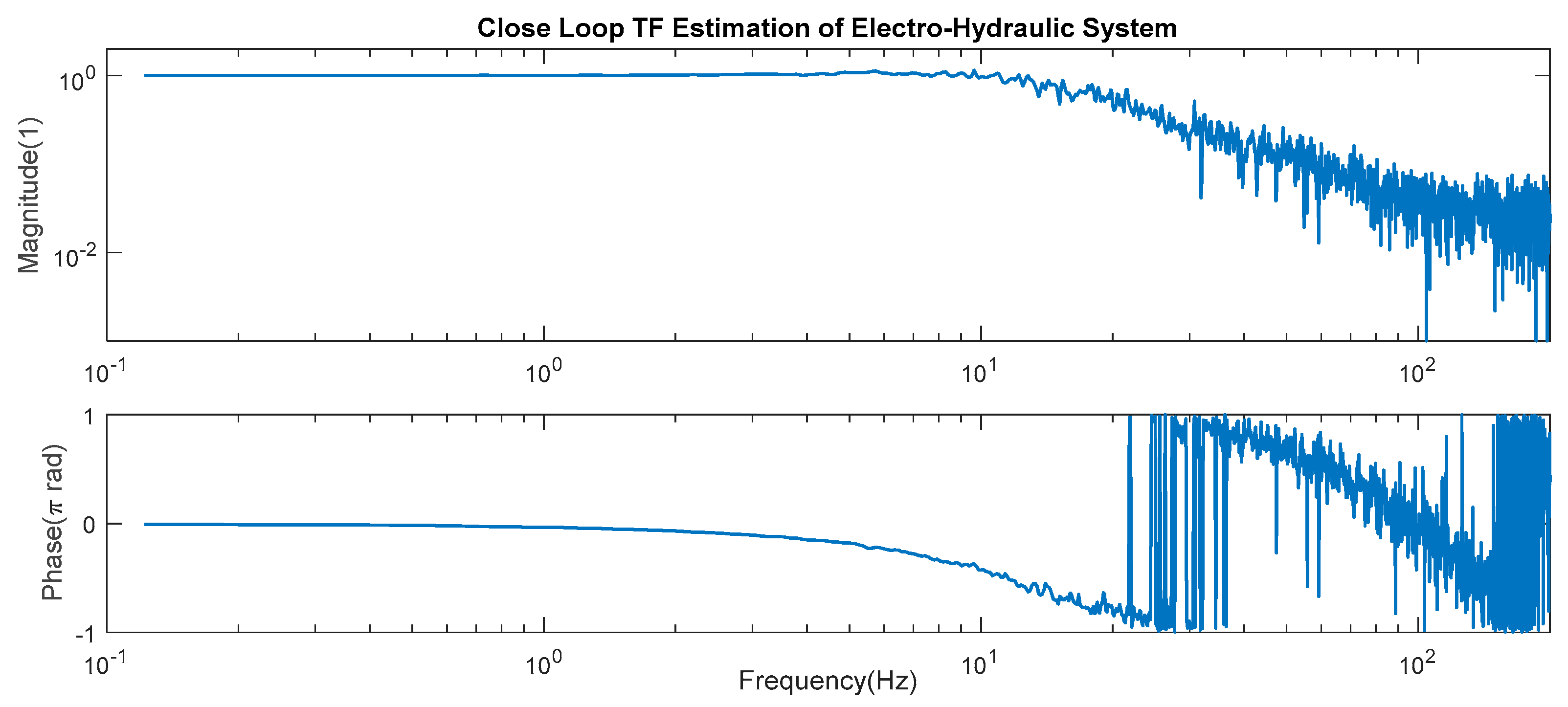
In order to better illustrate the characteristics of the experimental equipment, the image of the closed loop frequency domain TF of the experimental equipment used in this paper, namely the electro-hydraulic servo system, are displayed in Figure 8:

The closed-loop TF in the figure is the TF between the input displacement command and the piston displacement of the hydraulic cylinder collected by the sensor under the condition that the standard road is the input signal. It can be seen from the figure that in the important frequency range below 10Hz, the servo system's following characteristics are good enough to meet the requirements of the iterative experiment in this paper.

Different from the system under test in this paper, which is used to verify the iterative process, the electro hydraulic servo system, as an experimental equipment, has almost no change in its TF characteristics during the entire iterative process.

4.5. Standard Road and Real Road

The drive signal for linear TF estimate $H_L$ is virtual standard road noise, which can be seen as 0.1 power white Gaussian noise filtered by a Butterworth low-pass filter with one filter order and 0.1 rad/s band edge frequency.

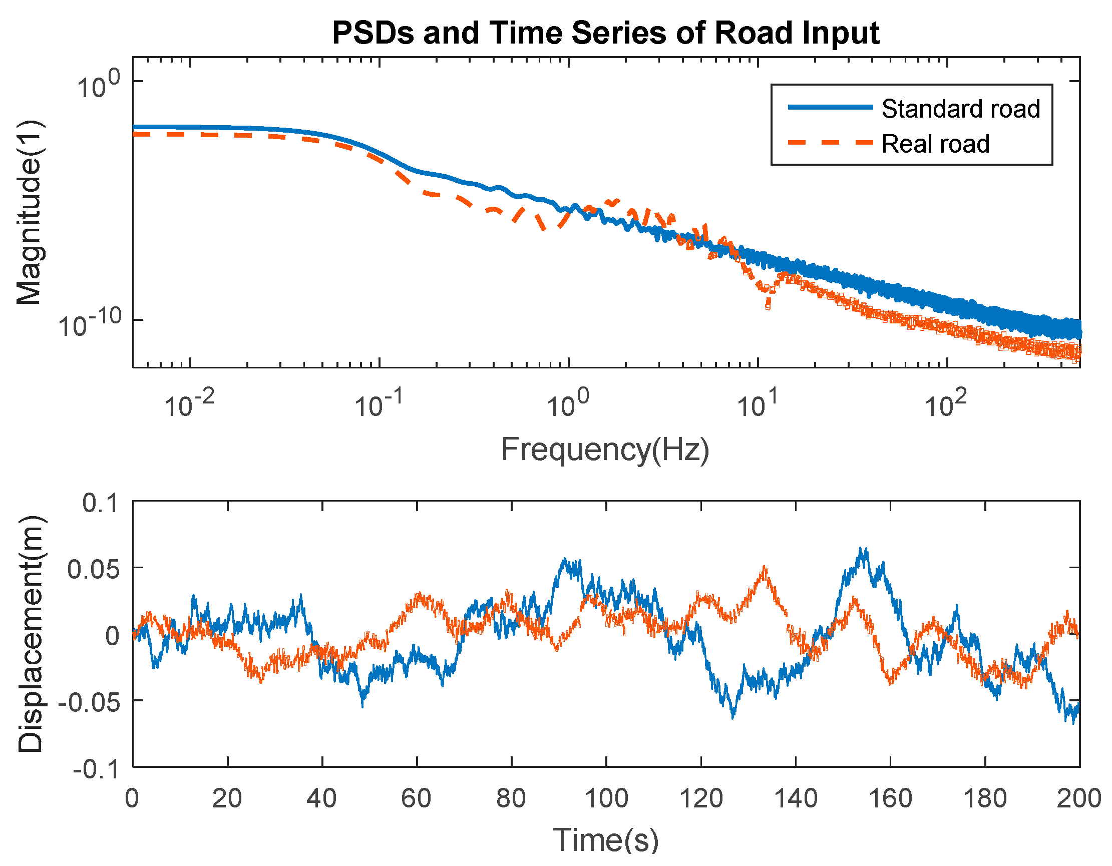
Based on standard ISO/TC108/SC2 [22], the standard road used in this paper is nearly between B-class road and C-class road. The vehicle speed in this paper is assumed as 10 m/s. Thus, after space PSD is transformed into time PSD, it is shown as the standard road line in the Figure 9:

Real road input can be seen as a shaped standard road, as shown in Figure. The real road is a commonly used concrete road in the small town, and has the best service status. The stand road and real road are called Road S and Road A, respectively.

The standard road is generated according to the standard and used to calculate the linear TF estimation of the system, while the real road is an actual road surface as an example for experimental verification. The bench test includes the test using the standard road as input and the test in the iterative process, while the real test uses the real road as input in this paper.

4.6. Control Strategies

In the experiment, five kinds of control strategies for iteration coefficient are used with notation of number 1~5, which are separately the modified strategy expressed in Section 3.2, simplified strategy expressed in Section 3.3, slow rise-up manual value, constant manual value and the RMS of NSRE-based manual value. The expressions of the iteration coefficient are shown below:

$$\frac{1}{{\mu }_{k,1}}=\Vert P_{k-2}+\frac{\partial H_{k-1}}{\partial D_{k-1}}{H}_L^{-1}{H}_{k-1}^{-1}{R}_0\Vert ,k\ge 2;\frac{1}{{\mu }_1}=\Vert P_0\Vert ;$$

(50)

$$\frac{1}{{\mu }_{k,2}}=\Vert P_{k-1}\Vert ,k\ge 1;$$

(51)

$${\mu }_{k,3}=\frac{2}{\pi }{\tan }^{-1}\left(\frac{k}{2}\right),{\mu }_{k,4}={\mu }_0,{\mu }_{k,5}={\mathrm{r}}_{k-1},k\ge 1;$$

(52)

The values of manual methods are based on the engineering experience [10,14,23], following several general principles below:

• The iteration coefficient is between 0 and 1;
• According to the actual system conditions, such as the degree of non-linearity, drive and acquisition characteristics, the iteration coefficient may need to be dropped, increased, or held constant;
• Experienced experimenter can also use current results to determine the iteration coefficient for the next iteration.

The control strategy 5 is a virtual experimenter who determines the next iteration coefficient based on the last RMS of NSRE.

5. Experiment Result

5.1. RMS of NSRE and Iteration Coefficient

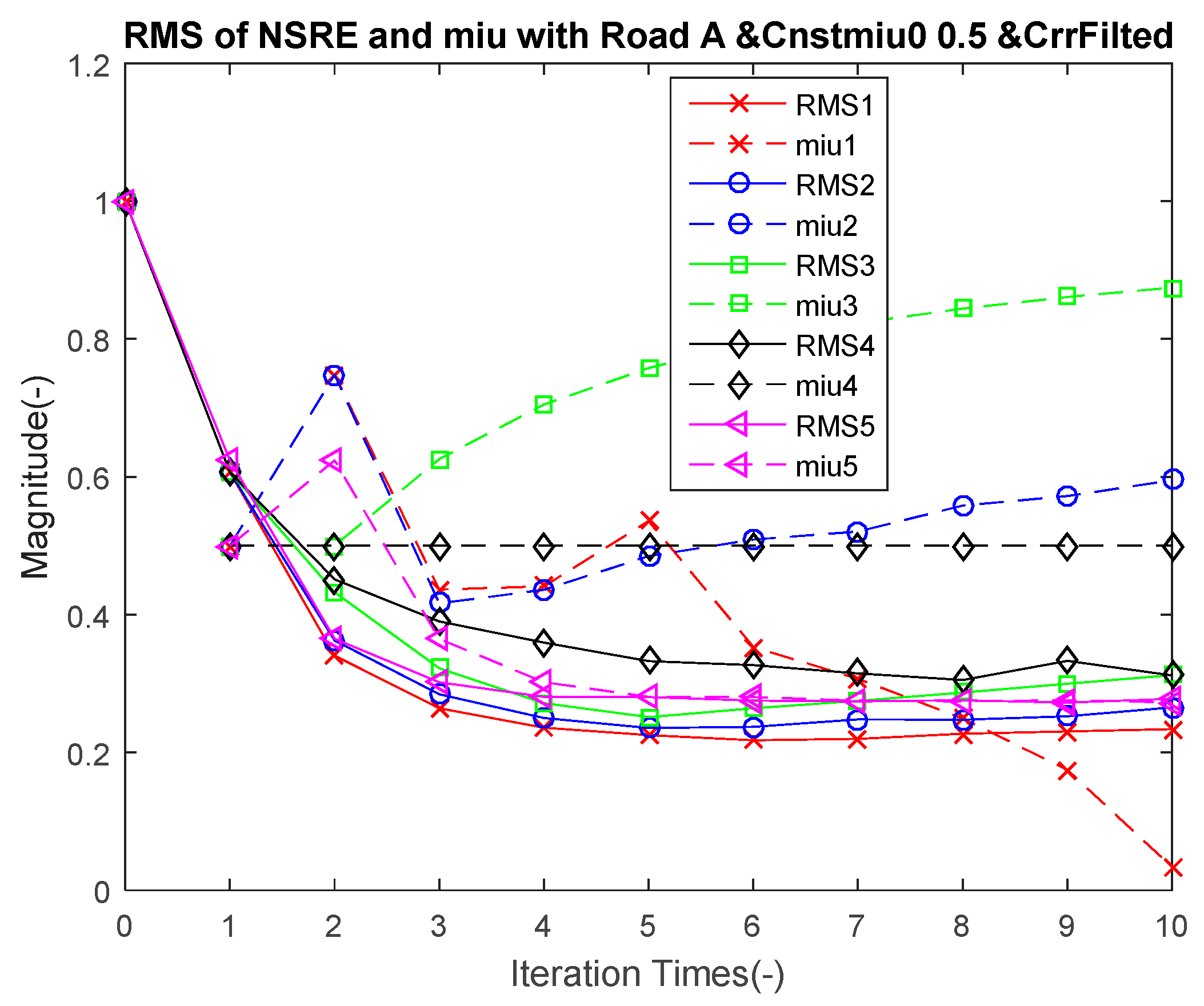
The RMS of NSRE of the iteration with modified strategy, simplified strategy, rise-up manual strategy, constant manual strategy and RMS based manual strategy, as well as the iteration coefficient ${\mu }_k$ are shown in Figure 10:

As shown in Figure and Table, the RMS of NSRE of the modified strategy namely method 1 is the best result, which has smallest minimum value and almost doesn’t diverge after the minimum point. The coefficient of the modified method is large at the beginning, then gradually decreases, and finally drops to very low. The result of the simplified strategy, namely method 2, is a little worse than the modified method, which has greater minimum than the modified strategy and slightly diverges after minimum point. Compared with the modified strategy, the coefficient of the simplified strategy still increases after minimum point of RMS of NSRE, which causes the divergence of the RMS of NSRE.

The RMS of NSRE of the rise-up manual strategy, namely method 3, diverges significantly after the minimum, and the minimum is larger than the modified and simplified strategies. The RMS of NSRE of the constant manual strategy, namely method 4, converges too slowly and the minimum is too large. The RMS of NSRE of the RMS based manual strategy, namely method 5, converges as fast as the modified strategy, but the minimum is much larger.

For RPC, with the progress of iteration, if the RMS value of NSRE can be stabilized at a relatively small value, then the iteration is considered to be convergent. The value of RMS is calculated based on the expression in Section 3.5, and related to the iterative control strategy, the experimental environment interference and the weighted characteristics in error evaluation.

The iteration results are listed in

Table 2. Iteration results.

Strategy No.	Minimum RMS (%)	Convergence Times	RMS of 10th Iteration (%)	Divergent Proportion (%)
1. Modified	21.76	6	23.41	0.4125
2. Simplified	23.57	5	26.55	0.5960
3. Rise-up	25.14	5	31.22	1.2160
4. Constant	30.54	8	31.19	0.7250
5. RMS based	27.42	7	27.80	0.1333

and

Table 3. Iteration coefficient and RMS of NSRE List.

k	1	2	3	4	5	6	7	8	9	10
miu1	0.5000	0.7481	0.4364	0.4411	0.5358	0.3532	0.3067	0.2493	0.1748	0.0337
miu2	0.5000	0.7481	0.4164	0.4361	0.4849	0.5089	0.5206	0.5583	0.5720	0.5949
miu3	0.5000	0.5000	0.6257	0.7048	0.7578	0.7952	0.8228	0.8440	0.8608	0.8743
miu4	0.5000	0.5000	0.5000	0.5000	0.5000	0.5000	0.5000	0.5000	0.5000	0.5000
miu5	0.5000	0.6238	0.3647	0.3021	0.2808	0.2804	0.2754	0.2742	0.2759	0.2726
RMS1	0.6069	0.3404	0.2640	0.2358	0.2251	0.2176	0.2199	0.2271	0.2304	0.2341
RMS2	0.6069	0.3622	0.2843	0.2501	0.2357	0.2371	0.2482	0.2476	0.2526	0.2655
RMS3	0.6069	0.4323	0.3223	0.2716	0.2514	0.2642	0.2751	0.2871	0.2998	0.3122
RMS4	0.6069	0.4511	0.3901	0.3593	0.3324	0.3269	0.3149	0.3054	0.3330	0.3119
RMS5	0.6238	0.3647	0.3021	0.2808	0.2804	0.2754	0.2742	0.2759	0.2726	0.2780

:

The minimum RMS is the minimum value of RMS of NSRE in the iterative process, and it is used to show the convergence accuracy of iteration. The smaller the minimum RMS is, the more accurate the iterative process.

The convergence times is the time number of the minimum RMS. It is used to show the convergence speed of iteration. The smaller the convergence times is, the faster the iterative process is.

The divergent proportion is the difference between the final RMS and the minimum RMS divided by the difference between the times of final iteration and the times of convergent iteration. The divergent proportion is used to show the stability of the control strategy. The smaller the divergent proportion is, the more stable the iterative process.

Although theoretically, the RMS of NSRE can converge to 0, while in practice, because of environmental interference and imperfect experimental equipment and system under test, RMS can only converge to a value greater than 0. In practical application, when the RMS value in the iterative process drops to a relatively small value and remains unchanged for two or three times of iterations, then it can be considered as the end of the iteration, which can be seen as the iterative convergence. Each strategy in this paper goes through 10 iterations in order to compare with each other and demonstrate stability, which is not necessary in practical application.

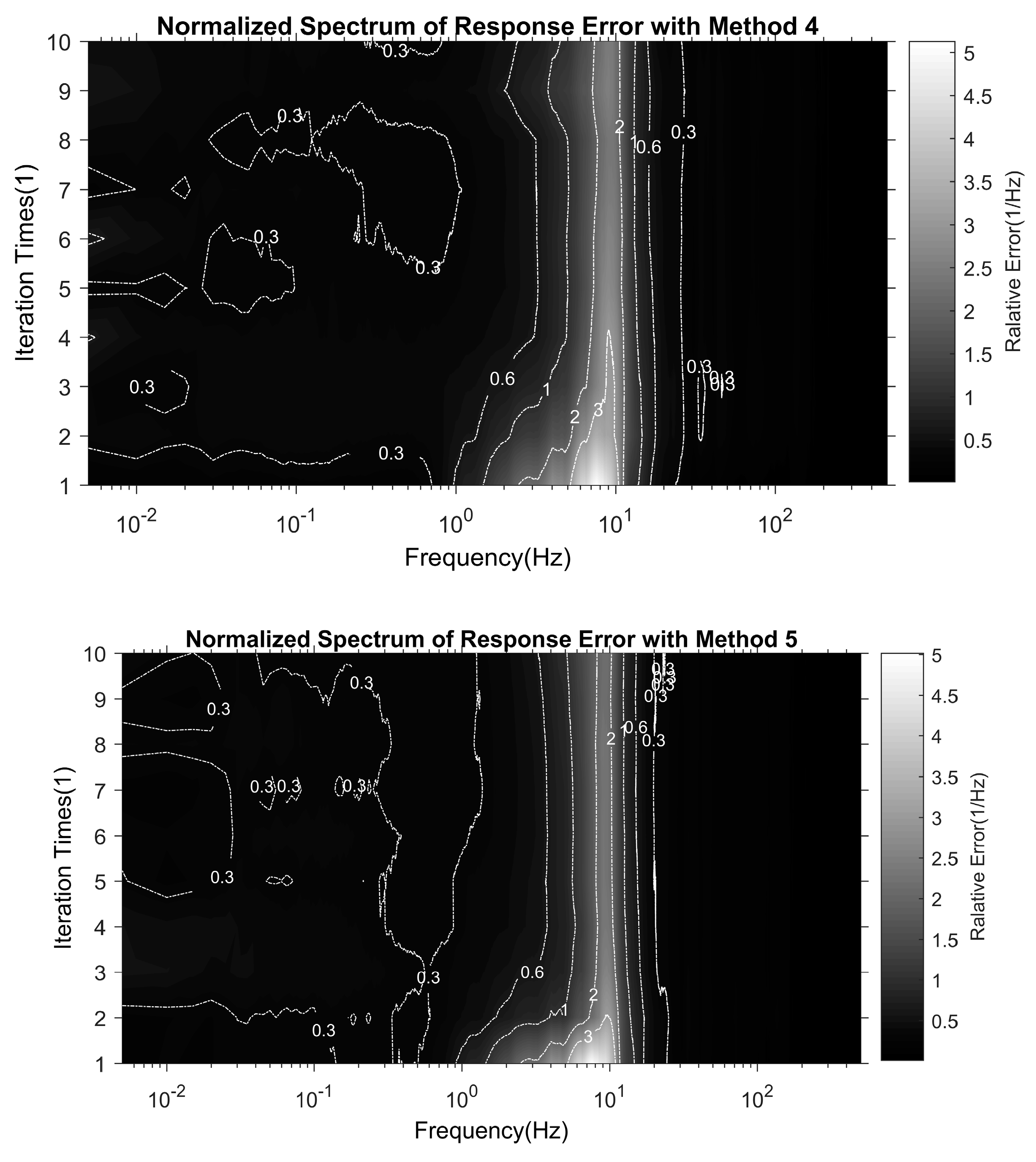
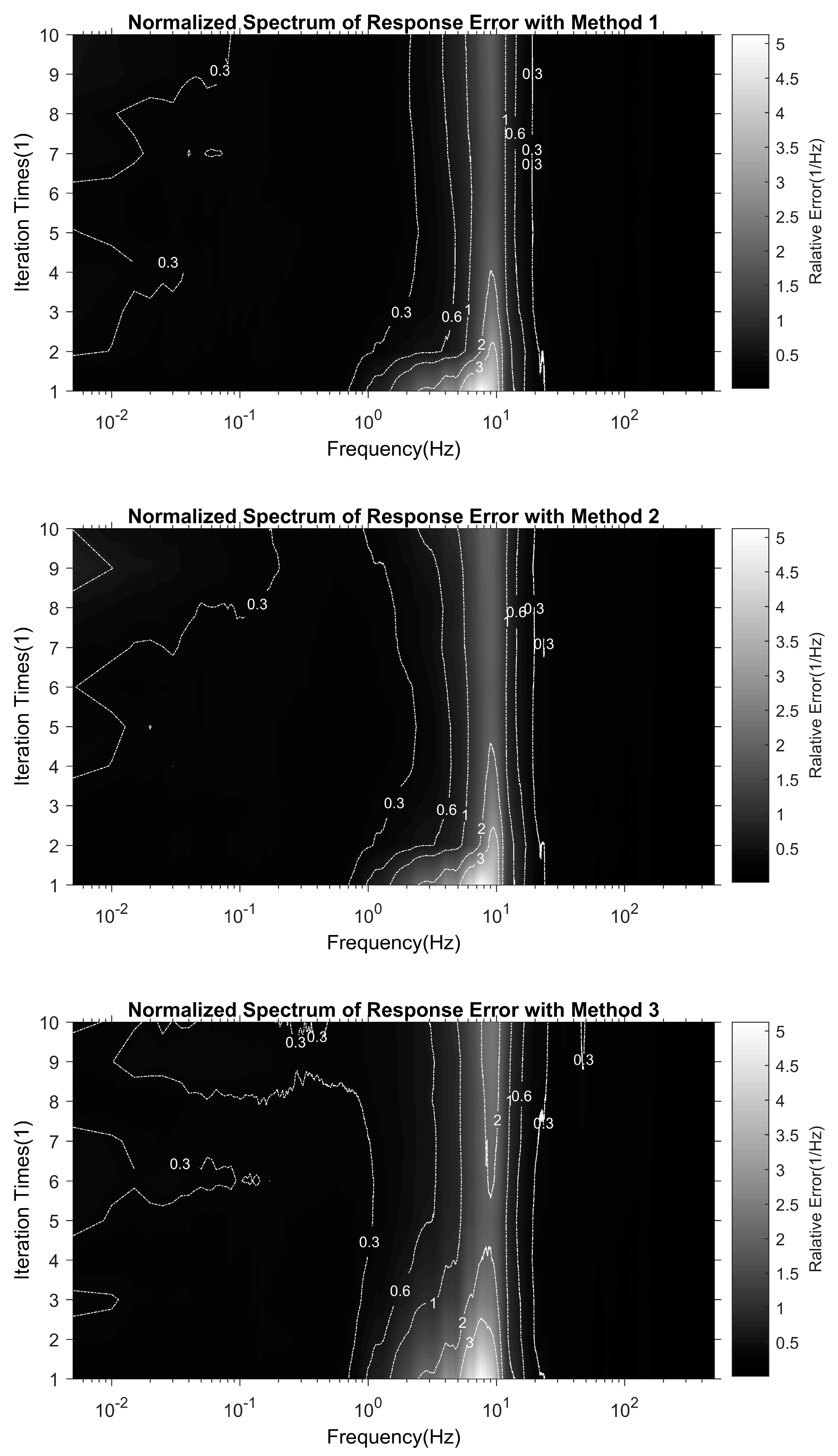
5.2. Iteration NSRE

In order to observe the change of response during the iteration under different control methods, the figures of NSRE with method 1–5 are shown in Figure 11 below:

As shown in Figure, the NSRE of the modified and simplified strategies, namely method 1 and 2, basically become smaller in the whole frequency range during the iteration process, while the rise-up strategy, namely method 3, gets bigger after the minimum point in both the low frequency and high frequency during the iteration process. The NSRE of constant manual strategy, namely method 4, and RMS-based manual strategy, namely method 5, also become smaller during the iteration process, but the values of NSRE in the whole frequency range are greater than the modified and simplified strategies.

It should be noted that, in the vicinity of 10Hz, the magnitude is relatively large from the beginning of iteration to the end of iteration, because 10Hz is the natural frequency point of the system, as shown in Figure 12. In addition, the nonlinear characteristics at this point (that is, the TF changes with the change of the iterative input) are also strong. Therefore, it is obvious at 10Hz in NSRE in the whole iterative process. However, as can be seen from the contour line, NSRE also decreased significantly at 10Hz, which is only highlighted by its large value.

The expression of NSRE is shown in Equation (47).

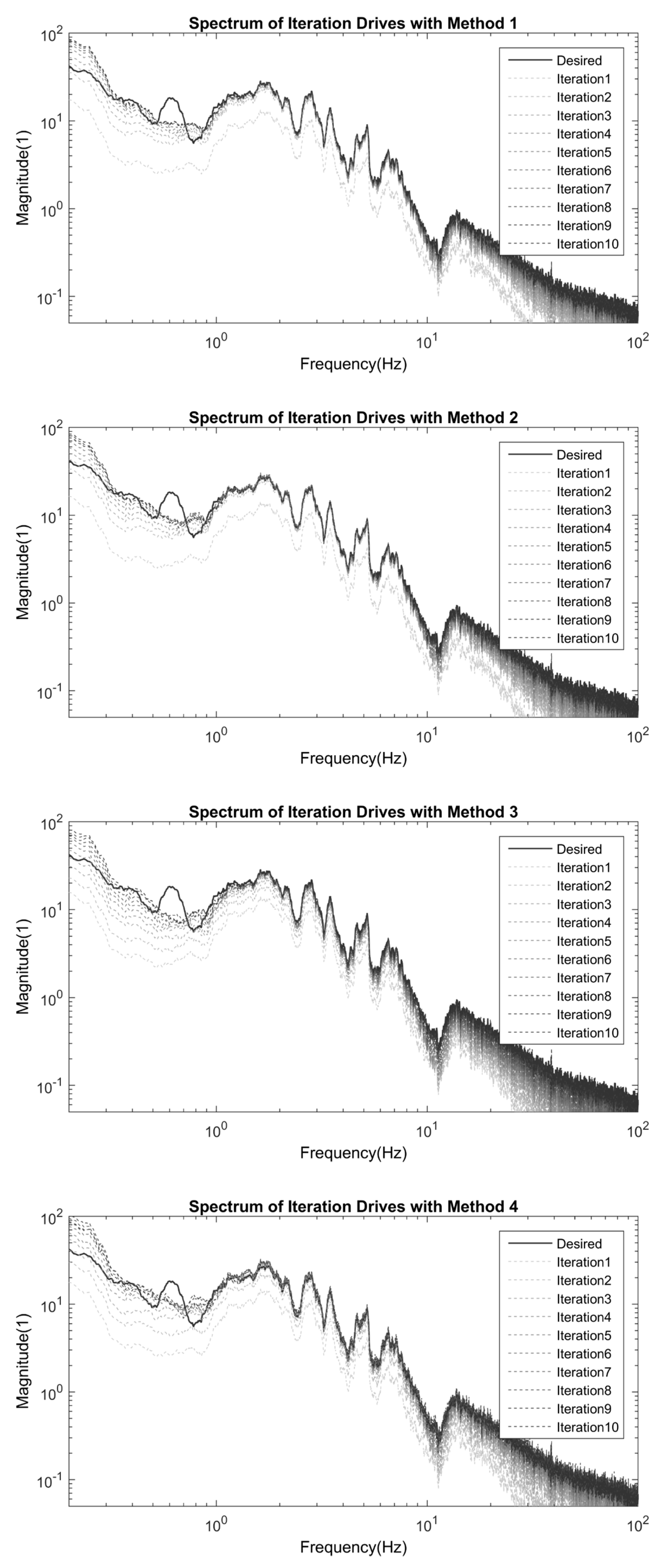
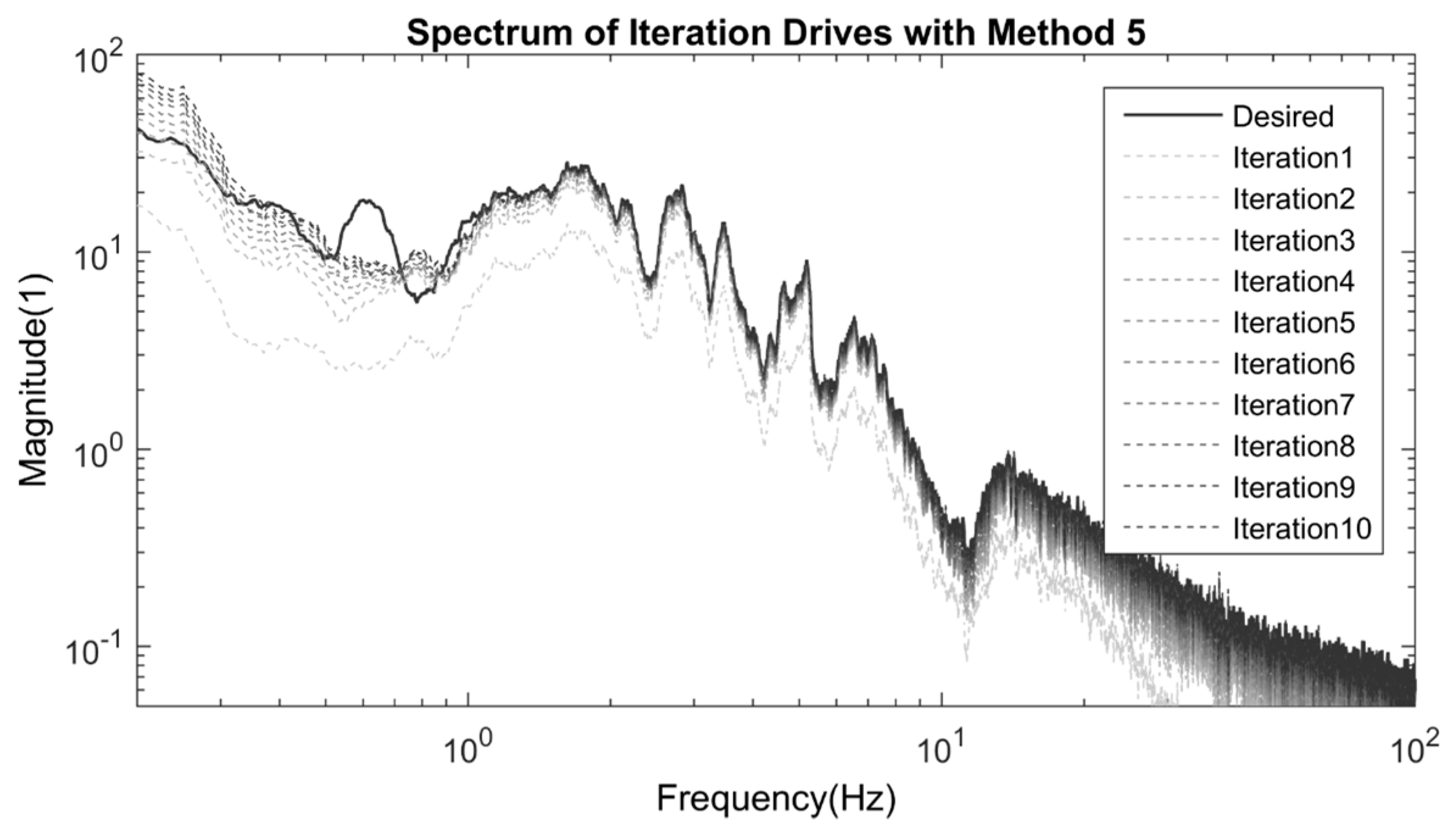
5.3. Iteration Drive and Road Drive Spectrum

In order to facilitate the observation of the change process of the drive signals in the iteration under different control strategies, the spectrum diagrams of the driving signals in the iteration are listed in Figure 12:

As shown in Figure, as the iteration progresses, the drive signal gets closer to the target signal (the road spectrum). The large deviation in the lower frequency band under 1 Hz is because the response of the whole system, especially the acceleration sensor, is poor in the lower frequency band. In the intermediate frequency part from 1 Hz to 10 Hz which is the most sensitive frequency range for human body vibrations [24,25], the drivers obtained by iteration are very close to the road spectrum. In the high frequency band above 10 Hz, because the amplitudes of driving signal and system response characteristics are very small, there are many burrs.

From the results obtained with different control strategies, the drive signal of method 1 and 2 is very close to the road spectrum only after 2 to 3 times iteration, and in the subsequent iterations, the drive signal does not deviate significantly from the road spectrum.

From the drive signal of method 3, it can be clearly seen that the driving signal needs at least 4 to 5 times of iteration before it could be closer to the road spectrum. Therefore, the convergence speed of method 3 is much slower than that of method 1 and 2. Although the drive signal of method 4 is very close to the road spectrum after 3 iterations, it is not stable around the road spectrum, but appears obvious overshoot phenomenon, so its stability is poor. The result of method 5 is similar to method 3, with slow convergence speed.

Although in Section 5.2, NSRE is always larger around 10Hz, because the system has certain nonlinear characteristics around here. It can also be seen from the system TF estimation in Section 5.5. However, as a precondition, the road spectrum itself has a relatively small amplitude around 10Hz, as described in Section 4.5. The drive spectrum in this section is still approaching the road spectrum gradually, without divergence or deviation at the natural frequency point of the system. Thus, the nonlinearity of the system at the natural frequency point does not cause the drive spectrum to diverge at a particular frequency point.

Therefore, it is proved that methods 1 and 2 can make the convergence process of iteration faster, more accurate and more stable. It means that the RMS of NSRE of iteration could reach the minimum quicker, the minimum RMS could be smaller, and the average increase rate of RMS after the minimum point could be smaller.

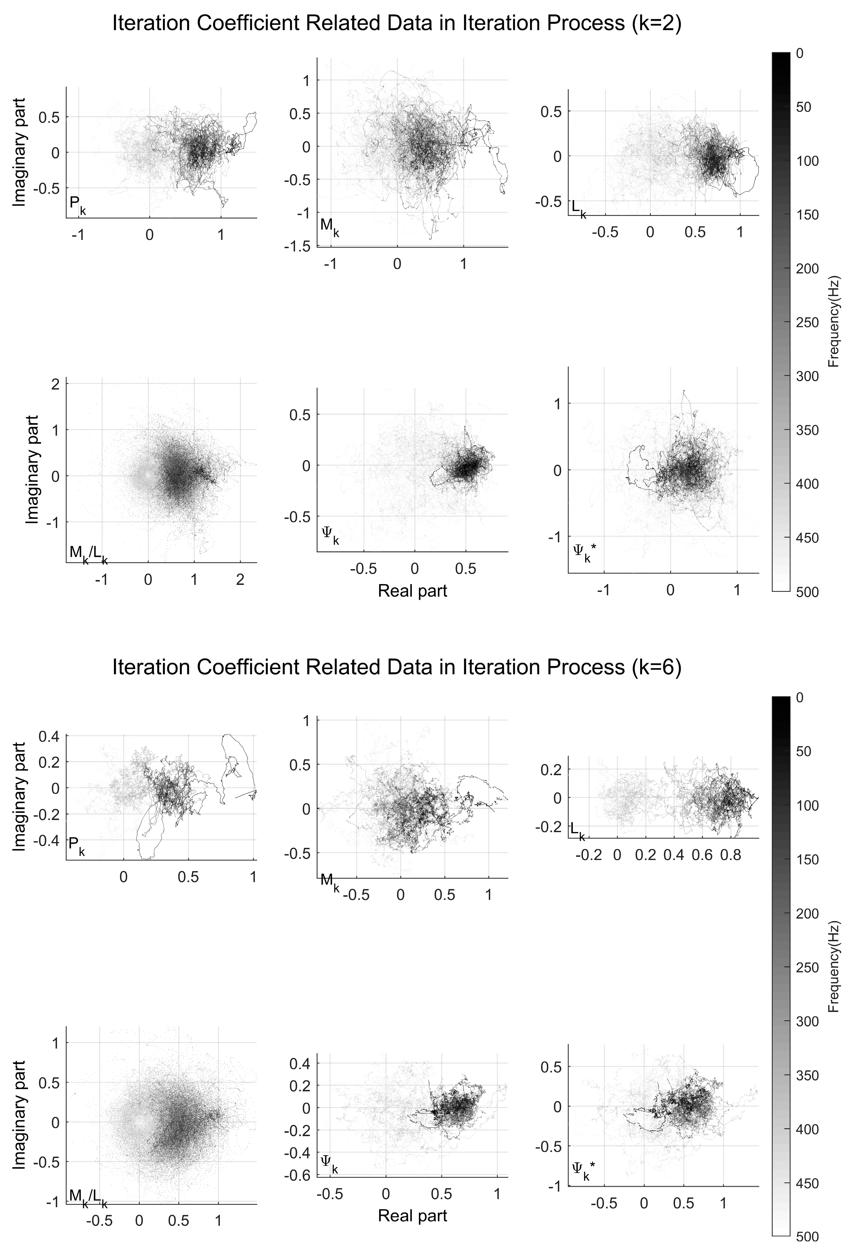
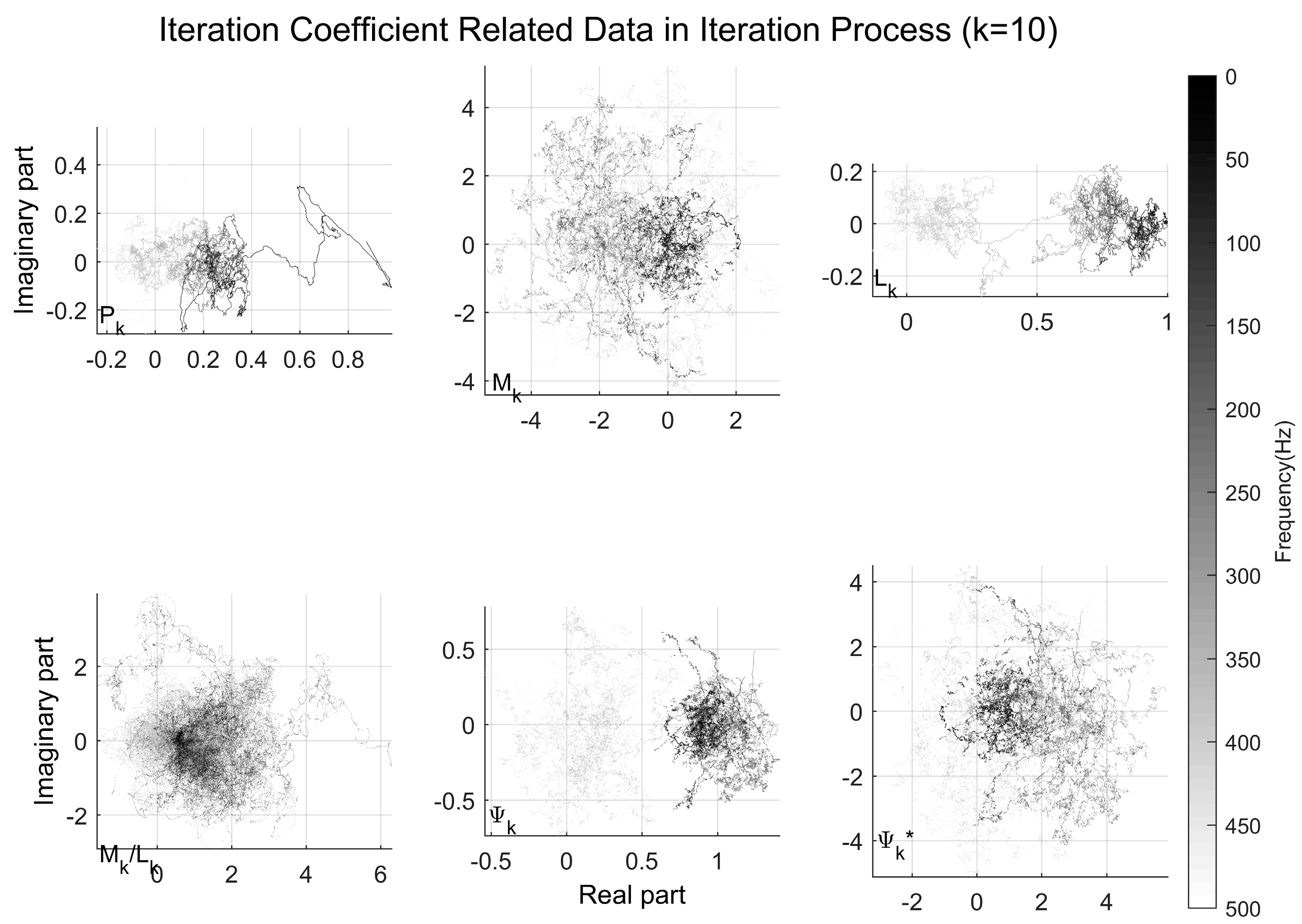
5.4. Iteration Coefficient Process Data

In order to verify the iterative process and the analysis of control strategy, the graphs of process data related to the iteration coefficient using control method 1 are listed in Figure 13 below:

The second, sixth and tenth iterations separately represent the early, middle, and late stage of the iteration process. The iteration process with modified strategy is chosen to verify the theory analysis of the control strategy.

As shown in Figure, in the early stage of iteration, the effective ratio ${ℳ}_k$ and TF ratio ${ℒ}_k$ are small and almost in the unit circle. The error ratio with iteration coefficient ${\Psi }_k$ and error ratio without iteration coefficient ${\Psi }_k^{*}$ are almost both in the unit circle, but the ${\Psi }_k$ is smaller than ${\Psi }_k^{*}$; in the middle stage of iteration. The ${\Psi }_k$ and ${\Psi }_k^{*}$ are a little bit out of the unit circle, but with the control of iteration coefficient, the ${\Psi }_k$ is still smaller than the ${\Psi }_k^{*}$. In the late stage of the iteration, the ${\Psi }_k^{*}$ is clearly beyond the range of the unit circle, but the ${\Psi }_k$ is still around the unit circle and still under control.

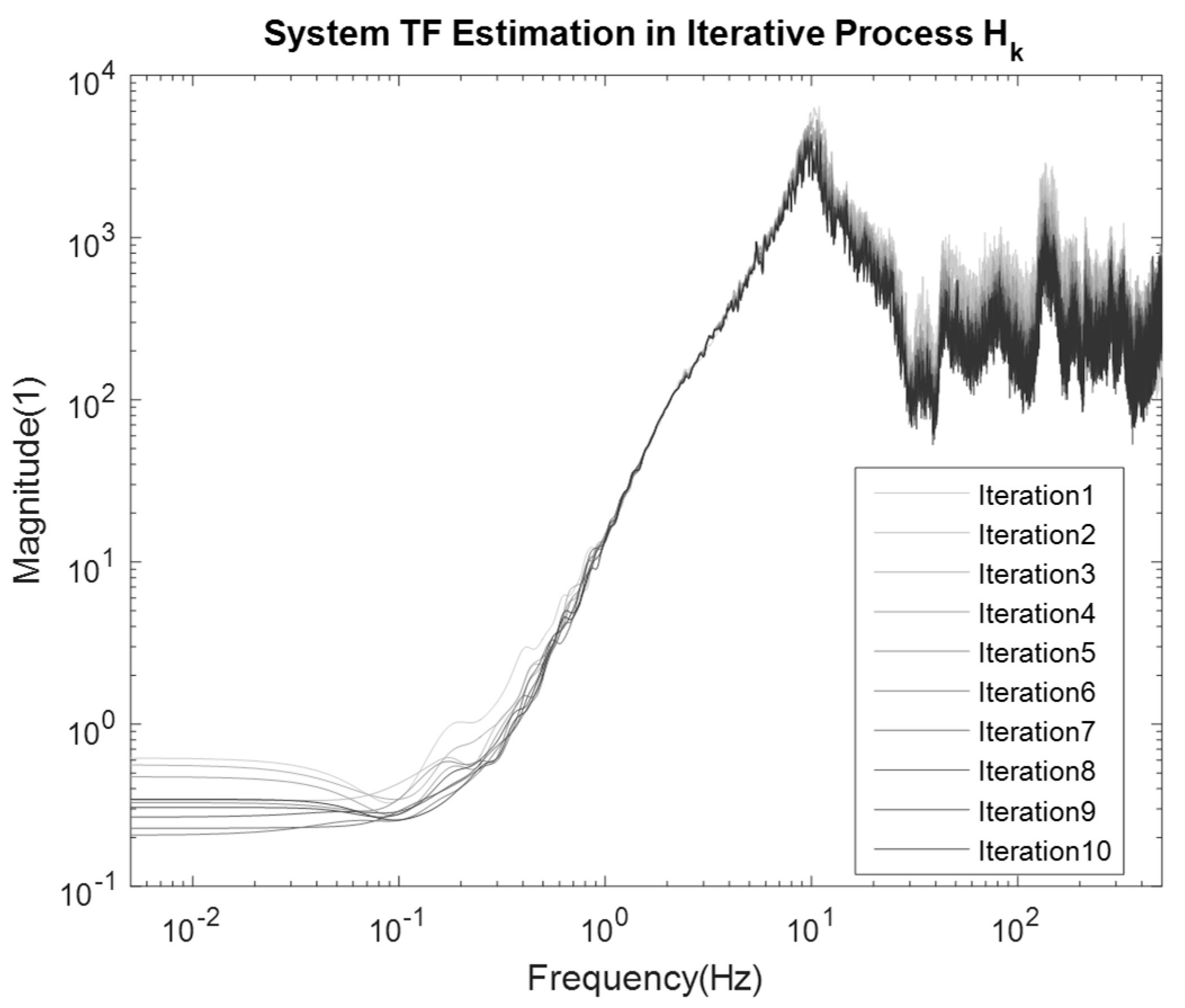
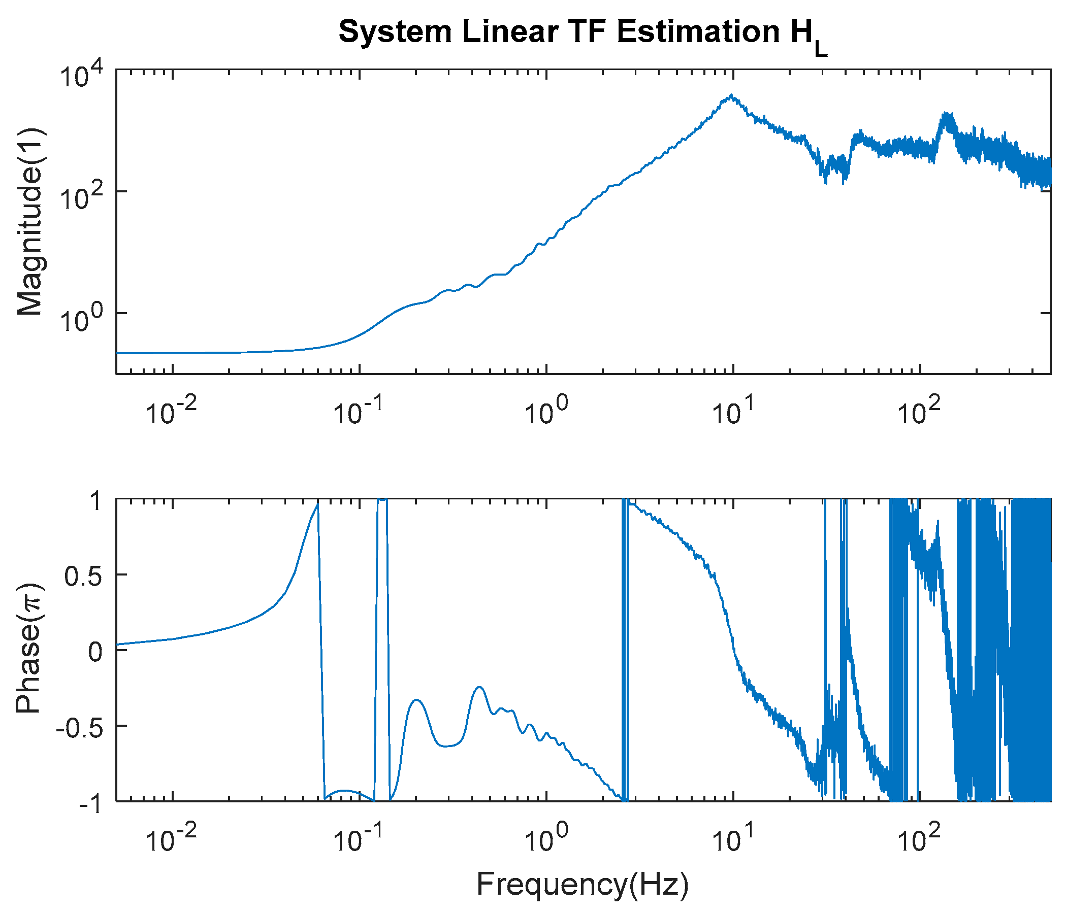
5.5. System Linear TF Estimation and System TFs

As shown in Figure 14, the magnitude of the linear TF of the system has an extreme point at 10 Hz, so the corresponding extreme point also has an extreme point at 10 Hz in NSRE.

Under the control of strategy 1, the system TF estimation of the iterative process is shown in Figure 15. Although the estimated iterative TF of the system is similar to the linear transfer function in general shape, the iterative TF of the system changes after each iteration, so it can be judged that the system is not completely linear.

The system linear TF estimation $H_L$ is shown in Figure as an initial estimation before the iteration. It is calculated with the standard road drive and the test response on the bench test. The system linear TF estimation $H_L$ used in iteration remains the same, while the system TF estimation in iterative process $H_k$ is variable and shown in Figure. According to the traditional RPC, the system linear TF estimation $H_L$ is used to calculate the drive correction with response error. The system TF estimation in iterative process $H_k$ is used to calculate the iteration coefficient based on the strategies proposed in this paper.

The system under test in this paper is the front part of the motorcycle, including wheel, suspension and frame; these components are nonlinear. The nonlinear characteristics of the vehicle under test will make the TF of the system under test vary with the input. In the iteration process, as the iteration progresses, the iterative input gradually approaches the real road. Therefore, when the iterative input keeps changing, the TF of the system under test will also change.

6. Discussion

The convergence speed in this paper is expressed by the time number of the minimum RMS. The convergence accuracy in this paper is expressed by the minimum RMS. The stability in this paper is expressed by the divergent proportion of the RMS. The divergent proportion is defined as the difference between the final RMS and the minimum RMS, divided by the number of last iteration and the number of iterations at the minimum RMS.

According to the figures and tables in Section 5.1, Section 5.2 and Section 5.3, method 1 converges slightly slower than method 2; however, the RMS minimum of method 1 is the smallest, so the convergence precision is the best, and the divergence ratio is smaller than method 2, which is relatively more stable. The convergence speed of method 2 is the fastest, but the minimum value is slightly larger than method 1, and the divergence ratio is larger than that of method 1, which is relatively more unstable. The method 3 converges at the same speed as method 2, but its minimum value is larg, and the divergence ratio is the largest, making it the most unstable. Method 4 has the slowest convergence, the largest minimum, the worst convergence precision, and a large divergence ratio—which is also very unstable. Method 5 has a slow convergence, a large minimum and a poor convergence precision.

Method 1 and method 2 have great advantages over manual strategy in convergence effect, convergence speed and iteration stability. The convergence effect of method 1 is the best, although the convergence speed of strategy 1 is not the fastest, the iteration stability is good. Compared with method 1, method 2 has the best convergence speed, but the convergence precision and iteration stability are slightly worse.

According to the figures in Section 5.4, the iteration coefficient can control the error ratio in the range close to the unit circle. In contrast, if there is no iteration coefficient involved in iteration control, the error ratio will be larger and larger as the iteration progresses, which will cause the iteration to diverge.

7. Conclusions

In this paper, the theory of RPC is expressed and analyzed step by step, and linear as well as nonlinear system conditions are considered. The convergence conditions of the iteration process on linear and nonlinear condition are discussed. Based on the convergence condition of iteration, the optimized control method for the iteration coefficient calculated by the vector norm is proposed. The method is modified and simplified to suit the real application.

In order to verify the correctness of the iterative process analysis and the applicability of the two control strategies, a light motorcycle is used as the device under test. Using the electro-hydraulic servo road simulation vibration bench as the experimental equipment, the iteration experiment is carried out. In order to compare the advantages and disadvantages of the strategies, three manual strategies are set up according to the engineering experience for the experiment. The manual strategies are rise-up, constant and RMS-based. The experimental results show that the analysis of the iterative process is practical and the control strategy serves the purpose of optimizing the iterative and convergent control.

The two control strategies proposed in this paper have different focuses. Method 1 focuses on convergence precision and iterative stability, while method 2 focuses on convergence speed. However, both control strategies are better than manual ones.

Compared with traditional manual methods determined by experienced engineer, the RPC iteration process with the optimized methods will converge faster and be more stable with less human involvement.

For a linear system and an ideal environment without interference, its TF does not change, and it naturally meets the iterative convergence condition of the linear system discussed in Section 2.2. Therefore, a good iterative process can be completed without the participation of the iteration coefficient. Since iterative parameters are not required, there is no need for iterative parameter calculation algorithm.

However, interference is inevitable for the actual test environment. And in modern vehicles, chassis, suspension, and tires are almost always nonlinear systems. Even if the system is still linear or nearly linear, it may not meet the convergence condition, so the iteration coefficient is needed to control the size of driving correction, so that the iteration process will not diverge. For traditional RPC, iteration coefficient is totally dependent on engineering experience and manual adjustment, which not only consumes a lot of time and human cost, but also may lead to unsatisfactory final results. Therefore, this paper proposes to discuss the convergence condition with the theoretical iterative process of the nonlinear system and calculate the iteration coefficient according to the convergence condition so as to achieve better and more cost-effective iteration effects than that of a traditional RPC.

We believe that the modification of traditional RPC based on the RPC iteration process of nonlinear system in this paper is original. And with the comparison experiment verification, it is confirmed that the improvement is valid, moreover has certain value to the practical application.

In this paper, the non-convergence problem of RPC iterative process is partially solved. For nonlinear systems, an iterative coefficient optimization method based on TF estimation is proposed according to the iterative convergence condition, which can make the iterative process meet the convergence condition and ensure the realization of convergence. At the same time, compared with the traditional manual parameter method, it has certain advantages. The reason for the iterative non-convergence of RPC is not only the nonlinear characteristics of the system, but also the external interference. Only the former is discussed in this paper. The influence of external interference on iterative convergence is not discussed in this paper due to the limitation of the research progress and paper length.

8. Limitation and Future Work

The control strategy in this paper depends on the TF estimation. According to the system under test, it may be necessary to adjust the filter parameters in detail according to the actual situation.

The purpose of simplification is to reduce the amount of computation, and from the results, the simplified strategy is also available. Due to the limitation of causality, the calculation process of the current iteration coefficient can only be performed with the last drive and response, so it may have some influence on the convergence speed and stability.

In this paper, the iterative convergence optimization of nonlinear systems is discussed, and the influence of external disturbances on the iterative process is not discussed.

If the control method needs to be extended to multichannel system in the future, a better multichannel TF estimation method is needed. For further improvement of the iteration coefficient, it is possible to improve the effect of the iteration coefficient on the convergence speed and stability of the iterative process by predicting the response of the system.