A Correlation-Change Based Feature Selection Method for IoT Equipment Anomaly Detection

Abstract

Selecting the right features for further data analysis is important in the process of equipment anomaly detection, especially when the origin data source involves high dimensional data with a low value density. However, existing researches failed to capture the fact that the sensor data are usually correlated (e.g., duplicated deployed sensors), and the correlations would be broken when anomalies occur with happen to the monitored equipment. In this paper, we propose to capture such sensor data correlation changes to improve the performance of IoT (Internet of Things) equipment anomaly detection. In our feature selection method, we first cluster correlated sensors together to recognize the duplicated deployed sensors according to sensor data correlations, and we monitor the data correlation changes in real time to select the sensors with correlation changes as the representative features for anomaly detection. To that end, (1) we conducted curve alignment for the sensor clustering; (2) we discuss the appropriate window size for data correlation calculation; (3) and adopted MCFS (Multi-Cluster Feature Selection) into our method to adapt to the online feature selection scenario. According to the experiment evaluation derived from real IoT equipment, we prove that our method manages to reduce the false negative of IoT equipment anomaly detection of 30% with almost the same level of false positive.

1. Introduction

In the era of the fourth industrial revolution, there is a growing trend to deploy sensors on industrial equipment, and analyze the industrial equipment’s running status according to the sensor data. Thanks to the rapid development of IoT technologies [1], sensor data could be easily fetched from industrial equipment, and analyzed to produce further value for industrial control at the edge of the network or at data centers. Due to the considerable development of deep learning in recent years, a common practice of such analysis is to conduct deep learning [2,3,4]. Such methods select a subset of all fetched sensor data stream as the input features, and generate equipment predictions. As a result, the performance of the learning model was seriously impacted by the features selected, thus feature selection plays a critical role for such methods.

To select an appropriate set of features for the learning model, researchers aim to select the most relevant features to the prediction model to improve the prediction performance, or to select the most informative features to conduct data reduction. Unfortunately, both kinds of methods have intrinsic drawbacks when applied in the online scenarios. The former kind of methods seriously depends on predefined evaluation criteria, such as feature relevance metrics [5] or a predefined learning model [6]. Thus, such method are limited to certain dataset, and are not suitable for online scenarios which involve dynamical and unsupervised feature selection. The later kind of methods right fits in the online scenarios. However, data reduction mainly aims to improve the efficiency (but not accuracy) of the prediction model, which is not the most concerning factor of online industrial equipment status analysis.

To relieve the dependency of predefined evaluation criteria, researchers switch to select the features which can indicate the online sensor data’s characters, such as features which are smoothest on the graph [7], or the features with highest clusterability [8,9]. In this paper, we focus on the features with correlation changes such as smoothness and clusterability, which are important characters for traditional pattern recognition fields like image processing and voice recognition [7,8,9]. We believe that correlation changes can significantly pinpoint status changes in industrial environment. As far as we know, this is the first work focusing on correlation changes for online feature selection.

In practical industrial scenarios, sensors catch equipment indicators that reflect various types of running status of industrial equipment. Because of the intrinsic mechanism of the industrial equipment, there exist prevalent correlations among equipment indicators. Herein, the corresponding sensor data streams are correlated. For example, as shown in Figure 1 are two sensor data streams collected from a coal mill in a thermal power plant, which indicates the power and coal flow of the coal mill over time. As the coal flow increases, the coal mill needs more power to digest the growing amount of coal, leading to the coal mill’s power increase. Accordingly, we can observe that the indicators of “power” and “coal flow” are correlated.

Sensor data correlations indicate the normal running of a set of equipment intrinsic mechanisms under certain running status. When the running status changes, the conditions supporting the equipment intrinsic mechanisms may break, and the running status changes may be reflected by the corresponding sensor data correlations. Considering that dynamic data correlations among industrial equipment sensors prevalently exist [10,11], we believe sensor data correlation change could be an effective metric for identifying the running status changes. Consequently, we propose to conduct online feature selection by selecting the sensors with data correlation changes.

To capture the sensor data correlation changes, the challenges include two-folds. The first problem is that industrial sensor data are always correlated with time lags [12]. This phenomenon makes the sensor data streams seem to be uncorrelated. As the example in Figure 1, because the coal mill needs a few minutes to grind the imported coal, the power of the coal mill does not increase as soon as the coal flow increases. In Figure 1, the two curves of “power” and “coal flow” have a time lag by about 3 min. When we compare the data segments of such two curves (as the square in Figure 1), there seems to be no correlation if we do not consider time lags.

The second problem is that industrial equipment sensor data analysis may involve tens of thousands of sensors, including huge amount of sensor data correlations to be taken care of, which leads to enormous online computation cost.

To solve the time-lagged correlation problem, we conduct curve registration to study the sensor data correlation. Considering the time lags are dynamic, we use dynamic time-wrapping methods to study the appropriate data segment for data correlation study. To solve the high-dimension problem, we conduct sensor clustering based on curve registration method to investigate the correlated sensors. By monitoring the correlation changes among correlated sensors, we manage to reduce the load of correlation monitoring.

In the rest of this paper, we first introduce few preliminaries of this paper in Section 2. In Section 3, we lay out the formal statement of our problem. We present the proposed methodology we propose in Section 4. We evaluate our methods with experiments in Section 5. We also compare our work with related works in Section 6 and conclude our work with comments on future research in Section 7.

2. Preliminaries

2.1. Correlation

Generally, there are two kinds of methods to quantify the correlations among time series data streams: the association rules and the liner correlation coefficient. The association-rules-based methods (e.g., frequent item mining methods) take the analyzed data as discrete items and analyze the temporal and spatial co-occurrence patterns of analyzed items as correlations. The liner correlation coefficient-based methods take the analyzed data as continuous value of variables, and focus on the comparison of the data value trend as correlation coefficient. The data value trend comparison is generally conducted on base of mathematical statistics [13] (e.g., Pearson Correlation Coefficient).

In terms of our problem, the equipment sensors kept generating continuous sensor values, and the data value trend was the key point. As a result, we relied on methods based on the liner correlation coefficient based methods, to study the correlation among sensor data streams.

2.2. Curve Alignment

When conducting correlation analysis on time series data sequences (curve correlation), if we consider no data sequence time lags, the correlations are prone to be misjudged (as shown in the example in Figure 1). To solve this problem, curve alignment methods [14] are proposed to align the time series data sequences when the two data sequences are correlated. Generally, curve alignment algorithms assume a consistent time lag for a pair of time series data sequences, and search for the optimal time lag with heuristic methods to maximize the data sequence correlation.

To our problem, for industrial equipment sensor data sequences, the assumption of consistent is too strong to be satisfied, and should be applied on a small piece of data segment.

2.3. Dynamic Time-Wrapping

Both curve alignment and dynamic time warping (DTW) [15] are methods used for measuring similarity between two time series data sequences. However, DTW methods do not make the assumption of a consistent time lag, and calculate an optimal matching between two given time series data with certain restrictions to maximize a measure of their similarity.

As for a long period of equipment data, we believe the time lags are dynamic which makes the curve alignment not accurate enough. Thus we use the dynamic time-wrapping method to compute the time lags over time (in the format of a series of time lags).

3. Problem Statement

Our feature selection problem takes a sensor data stream as the input feature sequence, and makes the feature selection decision at real time. As a matter of fact, the input sensor data are heterogeneous and multisource, especially in an industrial environment. However, we do not want to consider the ETL (extract transform load) problems, which are nontrival problems. Herein, in our online feature selection problem, we assume all sensor data streams arrive synchronously.

Let $x_1,x_2,\dots ,x_t,\dots$ denote the sequence of features, where $x_t\left(t=1,2,\dots \right)$ represents a $d$-dimentional data, noted as ($a^{\left(1\right)},a^{\left(2\right)},\dots ,a^{\left(d\right)}$), arriving at time $t$. Here, d is the quantity of the involved sensors, and also refers to the size of the feature space.

Our online feature selection problem aims at selecting a subset of the feature space, which includes the features with evident correlation changes. Formally, at each time t, we generate a feature subset $y_t$ which includes features like,

$$co{r}_{t-1}\left(a^{\left(i\right)},a^{\left(j\right)}\right)-co{r}_t\left(a^{\left(i\right)},a^{\left(j\right)}\right)>\epsilon ,1\le i,j\le d$$

(1)

Here $co{r}_t\left(a^{\left(i\right)},a^{\left(j\right)}\right)$ denotes the correlation metric between features $a^{\left(i\right)}$ and $a^{\left(j\right)}$ at time $t$, and $\epsilon$ is a predefined threshold for correlation changes.

Apparently, to monitor the correlation changes for each pair of features is a bad idea, especially when the feature space is on a large scale. Since we merely want to consider the correlation changes for the pair of features whose correlation reflect the equipment’s intrinsic mechanism. We just need to focus on the feature pairs which are always highly correlated according to the historical data, noted as correlated features. Herein, in Equation (1), $co{r}_{t-1}\left(a^{\left(i\right)},a^{\left(j\right)}\right)$ should be considered as close to 1, and we just need to make sure that $co{r}_t\left(a^{\left(i\right)},a^{\left(j\right)}\right)$ is small enough when selecting features $i\mathrm{and}j$, i.e., our problem is to monitor the correlations between correlated features pairs, and select the features pairs whose correlation is small enough, as shown in Equation (2).

$$co{r}_t\left(a^{\left(i\right)},a^{\left(j\right)}\right)<\epsilon ,1\le i\le d$$

(2)

4. Methodology

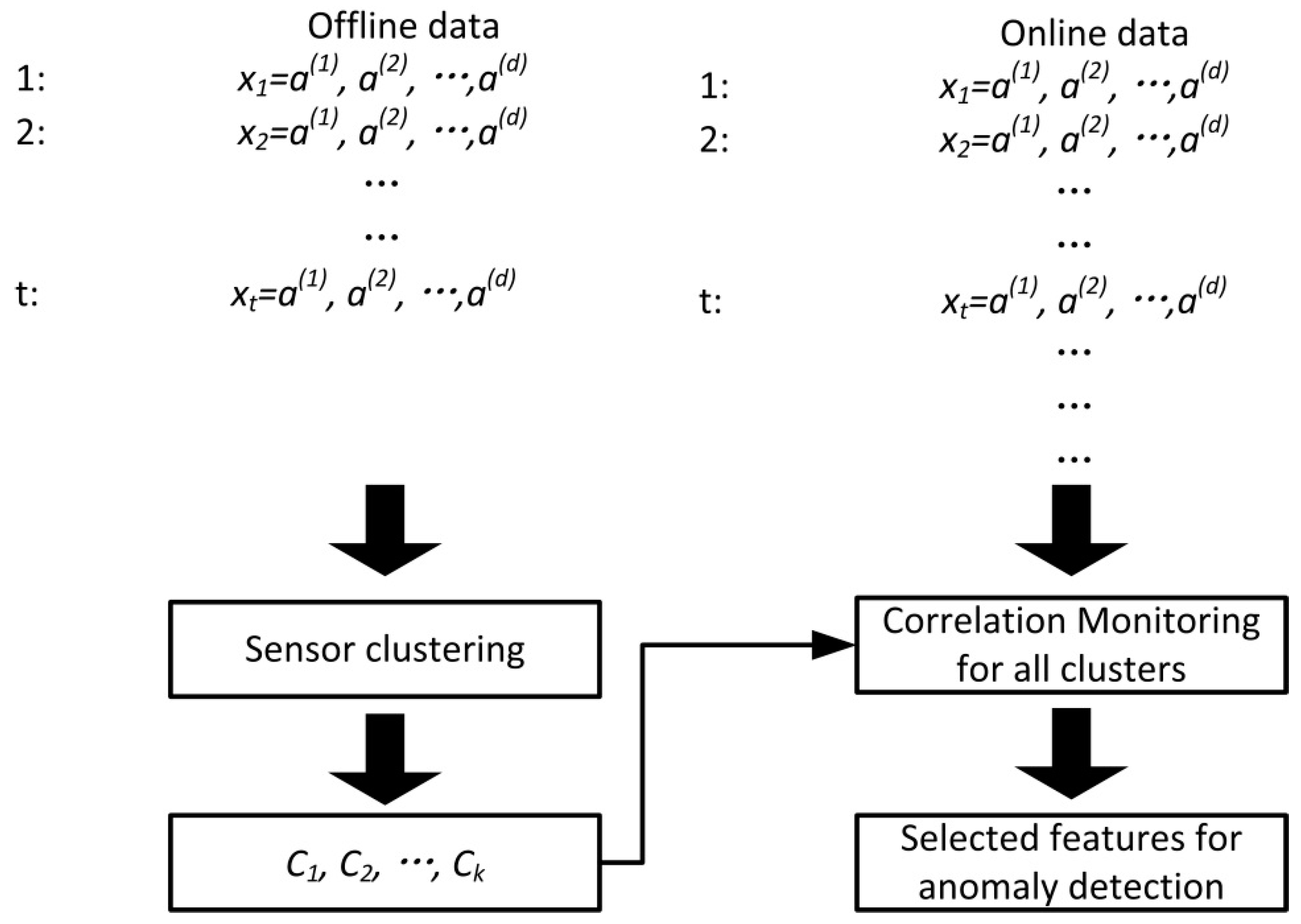
Figure 2 shows the overall workflow of our method. In the offline scenario, we clustered the sensors into groups according to the correlation of each sensor’s historical data, and the correlated sensors would be clustered into the same group. With the generated sensor structure, we monitored the data correlation within each cluster, and selected a set of representative features. A simple solution to our online feature selection is shown in Algorithm 1.

Algorithm 1. A simple algorithm for online feature selection.

Input: online feature sequence $x_1,x_2,\dots ,x_t,\dots$;

correlated feature set $C_1,C_2,\dots ,C_k$;

$\Delta$; #predefined correlation changes threshold

$seg$; #predefined data segment size for correlation calculation

Output: selected feature sequence $y_1,y_2,\dots ,y_t,\dots$;

1   For each arriving feature $x_t$

2       For each correlated feature set $C_l$

3          For each pair of features $a^{\left(i\right)},a^{\left(j\right)}$ in $C_l$

4              calculate $co{r}_t\left(a^{\left(i\right)},a^{\left(j\right)},seg\right)$;

5              if $co{r}_t\left(a^{\left(i\right)},a^{\left(j\right)},seg\right)<\Delta$

6                  add $a^{\left(i\right)}$ and $a^{\left(j\right)}$ into $y_t$;

7              End if

8          End for

9       End for

10  End for

According to the solution shown in Algorithm 1, we calculated the correlation for each pair of correlated features and selected that feature pair when the correlation is smaller than a predefined correlation threshold. Since Algorithm 1 needs the correlated feature set as input, we need to conduct feature clustering to generate the correlated feature sets according to the historical equipment sensor data. To cluster the correlated features together in our clustering method, we defined the similarity based on the feature correlations. We will discuss this in detail in Section 4.1.

The real time calculation of feature correlations (line 4 in Algorithm 1) needs to be further discussed in practice. The calculation of feature correlation is based on a piece of data segment of the two features. Since we wanted to capture the time-lagged correlation, we needed to conduct curve alignment to infer the time lags. Since the feature correlation is dynamic, we needed to conduct curve alignment based on the real time feature data. The size of the data segment is very important to our online correlation calculation. If the data segment is too big, the computation cost of online alignment would be considerable. On the contrary, if the data segment is even smaller than the time lag, we will have insufficient data to calculate the feature correlation. We will further discuss this in Section 4.2.

To enumerate all the feature pairs in the same feature set is also inefficient (line 3–8 in Algorithm 1). Considering a feature set $a^{\left(1\right)},a^{\left(2\right)},\dots ,a^{\left(h\right)}$ including h features, if only one feature (e.g., $a^{\left(1\right)}$) gets abnormal, the correlations between $a^{\left(1\right)}$ and $a^{\left(j\right)}j=2,3,\dots ,h$ will be small. According to Algorithm 1, the selected features will include all the h features in the feature set. Obviously, it is not necessary to involve all features because of merely one feature’s abnormal. As a result, we need a better representation for each feature set’s correlation changes. We will further discuss this in Section 4.3.

4.1. Feature Clustering Based Curve Alignment

One may argue the idea of feature clustering since the correlations of features transitivity is not strictly followed, i.e., features A and B are correlated; features A and C are correlated; but features B and C may not be correlated. In this case, there is no suitable partition for the clustering.

We admit the feature clustering may get a confusing result when the features transitivity is not strictly followed. However, according to our observation, in industrial environments, sensors are always duplicated when they are deployed. For example, to monitor the temperature of a bearing, there are always multiple sensors deployed from different angles on the same bearing. As a result, in normal cases, such sensors always get the similar data. As a result, in this paper, we assume that the feature correlation transitivity is strictly followed.

To conduct sensor clustering, we needed to define the similarity of a pair of features. Since we wanted to cluster the features that are highly correlated together, for each pair of features, we selected a set of historical data segments, and studied the feature correlations based on such data segments. If the two features are correlated on most of the data segments, we took the two features as correlated features, and combined them into the same cluster.

To capture time-lagged correlations among sensors, we conducted curve alignment when we studied the correlations of a pair of features, and made use of the SGEM (Smooth Generalized Expectation Maximization) [14] method to realize the curve alignment.

Formally, our method works as shown in Algorithm 2. We applied a hierarchical clustering based algorithm on the original feature space to cluster them into groups. Initially, we set each feature as a cluster. And we iteratively combine the clusters when they are correlated for most of the data segments according to the SGEM method’s output. Here, SGEM($D_k$, i, j) randomly selects a feature from cluster i and cluster j, and conducts SGEM method on data segment $D_k$ to generate the correlation coefficient and corresponding time lag. When no clusters could be further combined, we stopped our algorithm.

In Algorithm 2, we wanted to focus on the strong correlated features, therein we setup $\epsilon$ as 0.8 so that we only considered a pair of features to be correlated when their correlation coefficient is no smaller than 0.8. For the parameter ratio, since we simply want to combine highly correlated features, we setup ratio as 1.

Algorithm 2. Curve alignment based feature clustering algorithm.

Input: feature space $a^{\left(1\right)},a^{\left(2\right)},\dots ,a^{\left(d\right)}$;

Offline Data segments $D_1,D_2,\dots ,D_m$;

$\epsilon$; #predefined correlation threshold

ratio; #predefined ratio to correlated features

Output: feature clusters $C_1,C_2,\dots$;

1 Initialize all feature as a single cluster;

2 While (1)

3     For each cluster $C_i$ and $C_j\left(i\ne j\right)$

4         For each data segment $D_k$

5             $\left(timelag,cor\right)\leftarrow SGEM\left(D_k,i,j\right)$

6             If (cor > $\epsilon$)

7                 count++;

8             End if

9          End for

10           If ($count/\left|C_i\right|\left|C_j\right|$ $\ge$ ratio)

11              Combine clusters $C_i$ and $C_j$;

12           End if

13     End for

14     If (no clusters are combined in this iteration)

15           Break;

16     End if

17 End while

4.2. Dynamic Time-Wrapping for Data Segment Size

As we described in Section 1, the feature correlations are time lagged, and dynamic in industrial environment. Thus, to monitor the feature correlations online, we needed to conduct curve alignment at real-time. A critical problem here is to decide the data segment used online.

To that end, we looked into the historical data and investigated the historical time lag size. Curve alignment is a bad choice since it assumes consistent time lags for the data used for calculation. And we relied on the dynamic time-wrapping method, which considers dynamic time lags to find a time series matching which maximizes the curve similarity. With the result of dynamic time-wrapping, we could use the difference of each pair of matching time point to reflect the time lags over time. In this paper, we use the TADPole algorithm (Time-series Anytime DP) [16] to conduct our dynamic time-wrapping method.

To decide an appropriate data segment size, we wanted to ensure that the data segment size was bigger than most of the time lags. Herein, we assume the time lag of a pair of correlated features is a stochastic variable following normal distribution, and conducted parameter estimation for each pair of features to generate the mean and variance of normal distribution. Following the idea of statistical process control, normal time lags range from $\mu -3\sigma$ to $\mu +3\sigma$ ($\mu$ is the mean and variance is the $\sigma$). As a result, we choose $\mu +3\sigma$ as the data segment size for the pair of features because it is bigger size than most of the time lags.

Our procedure of data segmentation size works as shown in Algorithm 3. For each pair of correlated features, we used the TADPole method (line 3) to generate the time-lag sequence over the historical training data, and conducted statistical analysis (line 4) on the derived time lags sequence. Then we set $\mu +3\sigma$ as the data segment size for correlated features.

Algorithm 3. DWT-based data segmentation algorithm.

Input: feature space $a^{\left(1\right)},a^{\left(2\right)},\dots ,a^{\left(d\right)}$;

offline historical feature sequence $x_1,x_2,\dots ,x_t$;

correlated feature set $C_1,C_2,\dots ,C_k$;

T; #the set of historical training data

Output: Dsize; #the set of data segment size for correlated features

1 For each correlated sensor set $C_i$

2     For each pair of features $a^{\left(i\right)},a^{\left(j\right)}$ in $C_i$

3        $\Delta t\leftarrow TADPole\left(T,a^{\left(i\right)},a^{\left(j\right)}\right)$ # TADPole conducts TADPole algorithm on the offline historical feature sequence

4        $\left(\mu ,\sigma \right)\leftarrow stats\left(\Delta t\right)$;

5        $Dsize\left(a^{\left(i\right)},a^{\left(j\right)}\right)=\mu +3\sigma$;

6     End for

7 End for

One may argue that we don’t conduct dynamic time-wrapping in the previous step, which also calculated the similarity for a pair of features with a long period of historical data. This is because that dynamic time-wrapping methods merely focus on the matching of the time series but cannot be used to tell whether two time series are correlated.

4.3. Data Representation of Correlation Changes

In Algorithm 1, for a set of correlated features we would select all the features because of only one feature’s anomaly. Obviously, this is an inefficient data representation. To our mind, the selected features should be uncorrelated with each other, i.e., we need a low rank approximation to select the most informative features for each feature cluster when feature correlation changes happen. Fortunately, this has been widely discussed, and we conduct feature selection following the MCFS method [9]. The MCFS method analyses the feature correlation based on the recent feature sequence, and generates the important score for each feature. Based on feature importance, we select the dominant features with the largest scores.

Based on the above idea, we refine our feature selection algorithm as shown in Algorithm 4. For each feature set, we first conducted curve alignment (lines 6–11) to generate the time lags of all features. Then we applied the MCFS method to the feature sequence within the sliding window (line 12), and generated the dominant feature set as the selected features. It is noted that we do not conduct curve alignment for each pair of correlated features since we assume the features in the same feature set are highly correlated, and the time lags of feature pairs are consistent with each other. Herein, we just need a baseline for comparison. Without any correlation change, we can make a random selection. However, when there are correlation changes, we need to avoid the abnormal features since the time lag achieved by the SGEM method does not make sense. To that end, we selected the most dominant feature of the results of the MCFS method, because we believe that most of the features turn out to be normal, including the selected dominant feature, which is a safe choice for the baseline feature (line 13). After calculating the MCFS scores of each feature, we rank the feature importance according to the calculated MCFS scores from high to low, and select k features with the highest MCFS scores (line 15).

For Algorithm 4, we setup the parameter $\Delta$ as 0.2. Because we consider a pair of features not so correlated when their correlation coefficient is smaller than 0.8, if the correlation coefficient decreases more than 0.2, it has to be smaller than 0.8.

Algorithm 4. Feature selection based on feature importance.

Input: feature sequence $x_1,x_2,\dots ,x_t,\dots$;

correlated feature set $C_1,C_2,\dots ,C_k$;

$\Delta$; #predefined correlation changes threshold

Dsize; #the set of data segment size for correlated features

k; #the quantity of features to be selected

Output: selected feature sequence $y_1,y_2,\dots ,y_t,\dots$;

1 For each correlated feature set $C_i$

2     $\mathrm{make}\mathrm{a}\mathrm{random}\mathrm{selection}\mathrm{for}base\left[C_i\right]$;

3 End for

4 For each arriving feature $x_t$

5     For each correlated feature set $C_i$

6        $timelags=\left(\right)$;

7        For each pair of features $a^{\left(base\right)},a^{\left(j\right)}$ in $C_i$

8          $seg=Dsize\left(a^{\left(base\right)},a^{\left(j\right)}\right)$;

9          $\left(timelag,cor\right)\leftarrow SGEM\left(a^{\left(base\right)},a^{\left(j\right)},seg\right)$;

10           Add $\left(a^{\left(1\right)},a^{\left(j\right)},timelag\right)$ to $timelags$;

11           $\Delta T$ = seg if ($\Delta T$ < seg);

12        End for

13        $y_t^i=MCFS\left(C_i,timelags,t,\Delta T\right)$;

14        $base\left[C_i\right]=y_t^i\left[0\right]$;

15     End for

16     Select k features from all $y_t^i$ with the top k MCFS scores

17 End for

Figure 3 shows the revised workflow of our method. We first investigated the structure of the correlated sensors and the appropriate sliding window size used for correlation monitoring; then we utilized such a priori knowledge for online curve alignment. Finally, we used the aligned sensor data to conduct online feature selection.

Compared to the other dimension reduction methods, we believe the advantage of our method is that our offline learning procedure shrinks the range of dimension reduction computation. The existing works [17,18,19,20,21,22,23] conduct dimension reduction over all the sensors. However, our method focuses on the dimension reduction for each cluster, i.e., we ignore the possible dimension reduction for the uncorrelated sensor pairs. Such a difference could be quite obvious when there is a large number of sensor clusters and each cluster is not too big. We ignore the dimension reduction cross clusters because we believe the compressed information upon intrinsically uncorrelated sensors can hardly help the information representation of the raw sensor data.

5. Experiment Evaluation

In this section, we focus on the evaluation of our feature selection method by applying it to a real IoT equipment dataset for equipment anomaly detection.

5.1. Experiment Setup

Our dataset is learned from an open source dataset for anomaly prediction of wind-driven generator derived from a big data contest. The dataset includes stream data from 26 deployed sensors on wind-driven generators, including about 590,000 records of the running statement of two wind-driven generators over two months. Our dataset is also labelled with runtime blade icing problems indicating that anomalies occurred with the wind-driven generator.

We were unlucky with available datasets, since we were not able to get access to datasets that involve high dimensional data. However, as described in the following of this section, our dataset do involves issues with correlation changes that often run alongside equipment anomalies. In terms of discussing the effectiveness of our method, with high-dimensional sensor data, we conducted synthetic changes to our dataset to increase its data dimension.

Specifically, to generate a volume of sensor data, we randomly selected an existing data dimension (or select none of them, i.e., to generate a data stream that is totally independent to the real dataset) to generate a data stream that correlates with the selected data dimension (as shown in Algorithm 5).

Algorithm 5. Evaluation Data Set Generation.

Input: offline data stream $m_1,m_2,\dots ,m_d$;

$N$ quantity of features to be generated. Output: generated data stream $n_1,n_2,\dots ,n_N$;

1 For i = 0; i < N; i++

2    Generate random a, b, and c #c = 0, 1, 2, …, d

3    For each time stamp t

4       If c! = 0

5          Generate random $\Delta$ ($|\Delta |$ < $\left|b\right|$);

6          $n_i\left(t\right)$ = a∗$m_c\left(t\right)$ + b + $\Delta$;

7       Else if

8          $n_i\left(t\right)$ = b + $\Delta$;

9       End if

10    End for

11 End for

In this way, our dataset still had the characteristics such that the multiple data dimensions highly correlated with each other, and data correlation changes happen when the equipment anomalies happen. We randomly generated a few data streams because we wanted to generate noise data in the data set, so that we could apply our method to the generated data sets to prove the effectiveness of our method.

In the following, we use three datasets to conduct our experiments:

• Original: The original dataset we received from the big data contest.
• Wind-1000: We randomly generated 1000 data dimensions following our data generation plan, and the resulting dataset included 1026 data dimensions.
• Wind-5000: We randomly generated 5000 data dimensions following our data generation plan, and the resulting dataset included 5026 data dimensions.

In this paper, we compare our work with OPCA (Online Principal Component Analysis) [24] method which applies principal components analysis for feature extraction. We compare our method with OPCA because we believe that our method is able to capture the critical information for anomaly detection which can be easily omitted with normal data representation method. We conducted 200 tests, and generate the average performance as well as the standard deviation. For our experiments, the random factor is the structure of the clustered features and the initialized base of each cluster.

Our experiment environment is Ubuntu 16.04.1 LTS system, 64 bits, with 32 cores, 64G memory. Our deep learning tool is Keras [25] using Theano as backend. Keras is a neural networks API(Application Programming Interface) in Python, enabling us to use deep learning method to verify the effectiveness of feature selection method on failure detection.

5.2. Selected Features

Table 1. The impact of the number of selected features to the detection accuracy. The first row indicates the quantity of features we selected from our three datasets.

	5	10	20	30	40	80
Original	62.1 ± 0.2	72.3 ± 0.1	92.5	92.3	92.3	92.3
Wind-1000	60.4 ± 1.0	70.9 ± 0.4	86.1 ± 0.2	88.3 ± 0.1	89.2	89.3
Wind-5000	58.9 ± 2.1	69.1 ± 0.9	85.2 ± 0.5	87.3 ± 0.1	88.4 ± 0.1	88.6

shows is the impact of selected features to the overall detection accuracy. With the growing number of selected features, we are able to improve the detection result. For our original data set, the detection accuracy keeps improving until almost all selected features are selected. For Wind-1000 and Wind-5000, we are able to improve the detection result before we choose to select more than 40 features. Since the algorithm would also select features that are generated with no real information during our feature selection process, we have to select more than 26 features to improve the feature selection effectiveness. The upper-bound is about at the level of 88%. It is noted that our method is able to improve the detection accuracy to almost the same level of the original data set, indicating that our method is able to select a similar set of features that are useful for the anomaly detection. The totally necessary quantity of features is about 30–40 features to get an optimal result, which about 1.5 times the feature sets of the original data set. But if we take 85% as an acceptable detection result, we are able to do that with a set of 20 features. We believe the gap between Wind-1000 and Wind-5000 to the original data set is due to the noise we randomly generate, and the difference is 3–4% in our evaluation. It is also noted that the standard deviation of our method on 3 datasets are all very small, because the random factor in our experiment is quite trivial. The only case that may impact the accuracy is that we select the sensor that is abnormal, and conducting curve alignment with such a base would induce inaccurate detection result.

5.3. Detection Accuracy

Next, we compared our method with the Online PCA by applying OPCA to our data sets. Here we set the selected features as 15. As shown in

Table 2. The comparison of our method with the OPCA method on false positive rate.

	Our Method	OPCA
original	9.4	12.4
wind-1000	16.7 ± 0.2	14.1
wind-5000	18.3 ± 0.6	16.4

is the false positive rate of our anomaly detection results. It is noted that the false positive rate of the two methods is basically at the same level. For the original data set, our method performs better than OPCA. However, for the two bigger datasets with noise data, OPCA express its advantage in filtering noise data, and performs better than our method.

As shown in

Table 3. The comparison of our method with the OPCA (Online Principal Component Analysis) method on false negative rate.

	Our Method	OPCA
original	22.4 ± 0.2	54.1
wind-1000	28.7 ± 0.5	60.6
wind-5000	31.3 ± 1.2	65.2

is the false negative of our anomaly detection results. Different from false positive rate, for all 3 data sets, our method outperforms the OPCA method. The false negative rate of our method is at the level of 20–30%. However, the false negative rate of the OPCA method is at about 50–60%. As a matter of fact, our method works better because the data set corresponds to our assumption that the anomalies come along with the correlation changes. Among all the equipment failures, 28.9% of such failures come up with a correlation change, and our method manages to capture all such equipment failures. Our experiment results also indicate that correlation changes cannot be accurately captured by the PCA method. A PCA method aims at getting the most informative features which can almost represent the original data, which has no deal with correlation change.

6. Related Works

During recent years, with the growing interest on deep learning methods [26,27,28,29,30] and wireless sensor networks [31,32,33,34,35], the feature selection methods are drawing more and more research attention. The existing feature selection methods could be classified into two types, namely, batch methods and online methods. Based on the selection criterion choice, the batch methods can be roughly divided into three categories: filter, wrapper and embedded methods. Filter methods [36] are in independent of any earning algorithm, and relies on evaluation measures such as correlation, dependency, consistency, distance and information to select features. A wrapper method [6] performs a forward or backward strategy in the space of all possible feature subsets, using a classifier of choice to assess each subset. Generally, this method has high accuracy and can search the feature suitable for the predetermined learning algorithm, but the exponential number of possible subsets makes the method computationally expensive. The embedded methods [37] attempt to simultaneously maximize classification performance and minimize the number of features used based on a classification or regression model with specific penalties on coefficients of features. The embedded methods aim to integrate feature selection process into model training process. It can provide suitable feature subset for the learning algorithm much faster than the wrapper methods, but the selected features may be not suitable for other learning algorithms.

In spite of the massive research on feature selection, most of them need a pre-learning process, which cannot be easily scalable for high dimensional data analytics that require dynamic feature selection. Hence, many online feature selection methods have been proposed, which can be classified into two research lines. One assumes that the number of features is fixed while the number of data points changes over time [17]. Wang et al. [18] proposed an Online Feature Selection (OFS) method, which assumes data instances are sequentially presented, and performs feature selection upon each data instance’s arrival. Wu et al. [19] presented a simple but smart second-order online feature selection algorithm that is extremely efficient, scalable to large scale and ultra-high dimensionality. The other online assumes that the number of data instances is fixed while the number of feature changes over time. Perkins et al. [20] firstly proposed the Grafting algorithm based on a stage wise gradient descent approach for this kind of online feature selection. It treats the suitable features selection as an integral part of learning a predictor in a regularized learning framework, and gradually building up a feature set while training a predictor model using gradient descent in an incremental iterative fashion. Zhou et al. [21] presented Alpha-investing which sequentially considers new features as additions to a predictive model by modeling the candidate feature set as a dynamically generated stream. However, Alpha-investing requires the prior information of the original feature set and never evaluates the redundancy among the selected features as time goes. Wu et al. [22] presented Online Streaming Feature Selection (OSFS) algorithm with a faster version, the Fast OSFS algorithm. The computational costs of above methods are very expensive or prohibitive when the dimensionality is extremely high in the scale of millions or more. Yu et al. [23] presented Scalable and Accurate Online Approach (SAOLA) algorithm, a scalable and accurate online approach, to tackle the feature selection with extremely high dimensionality. It conducted a theoretical analysis and derived a lower bound of correlations between features for pairwise comparisons, and proposed a set of online pairwise comparisons to maintain a parsimonious model over time. To sum up, the existing researches of online feature selection seldom focus on the correlation changes, thus fails to capture the characteristics of correlation changes. This leaves a large space to be improved upon in terms of prediction accuracy.

7. Conclusions

The high-dimensional data for industrial sensor data analysis and time-lagged correlation among sensors result in challenges to build an accurate predictive model for IoT equipment anomaly detection. In order to select effective features from massive high-dimensional sensor data with time-lagged correlation, this paper presents a correlation change-based feature selection method for online feature selection. We applied our proposed method to a real case data set, and proved our method is able to capture the effective features for anomaly detection which PCA-like methods are unable to cope with. As a future work, one could apply our method on a bigger dataset to prove the ubiquity of sensor correlation changes in equipment failures. It is also valuable to refine the data flow of our method to make the parameter setup iteratively refine according to the sensed equipment context.