1. Introduction
With the advancement of renewable energy technologies and the rising enthusiasm for environmental protection, various countries have proposed energy strategies emphasizing the increase of renewable energy power generation to reduce reliance on fossil fuel power generation. According to the latest Renewable 2018 Global Status Report released by the Renewable Energy Policy Network for the 21st Century, total renewable power capacity reached 2195 GW by the end of 2017, with wind power accounting for the highest proportion (539 GW), followed by solar photovoltaics (PV) at 402 GW [
1].
The Taiwanese government has actively promoted the development of renewable energy in recent years, planning to achieve a total of 27 GW renewable power capacity by 2025, which will account for 20% of the total power capacity and will include 4.2 GW of offshore and onshore wind power and 20 GW of solar PV. The government also proposed two-year and four-year implementation projects for solar PV and wind power generation, respectively. The short-term goal comprised a total installed capacity of PV of 1520 MW and cumulative installed capacities of onshore and offshore wind power of 814 and 520 MW, respectively [
2].
In the traditional unit commitment (UC) problem, the startup and shutdown times of various units and the power output within a dispatch time period of 1 day to 1 week or even 1 month to 1 season are planned according to the system load to achieve the lowest operating cost. In addition, with the load requirement being satisfied, the traditional unit commitment problem ensures that the criteria for the operation of each unit can be met. These criteria include the upper and lower limits of power output for each unit, the ramp rates of the units, and the balance between the supply of and demand for electricity. However, because of the intermittent characteristic of renewable energy, the power output may substantially decrease or increase within a few minutes due to weather events (such as an eclipse, no wind, or strong wind). Such circumstances are typically managed by using pre-established spinning reserves and storage systems [
3]. However, all these methods require additional costs and are unable to effectively use renewable energy.
Some studies on the ramp rate of power generating units after the integration of renewable energy into the system are described as follows. Correa-Posada et al. used a dynamic ramping model, namely mixed-integer linear programming, which considered the flexibility of ramping limits to reduce the dynamic errors caused during ramping [
4]. Ding and Bie used the IEEE 118 bus as an example; the Lagrangian relaxation method was integrated with the diagonal quadratic approximation method to solve the dynamic economic dispatch optimization problem after consideration of the unit ramp rate [
5]. Haaren et al. controlled the rapidly changing ramp rate caused by the integration of a large-scale photovoltaic system into the electrical grid. The authors integrated an ultracapacitor (Maxwell), two flywheels (Beacon Power), and two batteries (Li-ion and Lead Acid) to effectively control the power output of solar energy to prevent frequency changes from destabilizing the system [
6]. Saka et al. considered transmission losses, ramp rate limits, and prohibited operating zones, and used the vortex search algorithm for scheduling the economic load dispatch problem [
7]. Correa-Posada et al. also applied the mixed-integer linear programming to the unit ramp rate constraint to effectively allocate operating reserves to thermal units, especially gas-fired generators [
8]. Wanga et al. proposed an optimal dispatching strategy for the dispatch of the power system during peak load periods under high wind power penetration and rapid ramp events. In that study, the prediction of wind power rapid ramp events and spinning reserve procurement were used as the conditions for analysis [
9].
Optimization algorithms based on stochastic searching methods have been widely used for the unit commitment problem, including exhaustive attack methods, Lagrangian relaxation methods, conventional quadratic programming (QP), branch and bound (B&B), artificial neural networks (ANN), simulated annealing (SA), and improved particle swarm optimization (IPSO) [
10,
11,
12,
13,
14,
15,
16,
17]. The exhaustive attack method is a brute-force algorithm, which is used to obtain all the possible solutions for comparison and then further determine the optimal solution [
10]. However, if all possible combinations are used for calculation, the curse of dimensionality may occur, preventing the search from discovering the optimal solution and compromising solution quality and calculation time. According to Lagrangian relaxation method, the constraint for the minimum problem is multiplied by the Lagrange multipliers, and the product is incorporated into the objective function to convert the problem into a dual maximization problem that can be easily solved. Although the solution can be easily obtained, the problem-solving requires a simplified cost curve and thus may produce inaccurate solutions. Inappropriate selection of the initial value may also result in oscillation or even divergence [
11]. Conventional quadratic programming can convert a complex nonlinear restriction programming problem into an easily solved sequence quadratic programming subproblem, but is limited to problems written in terms of linear equations and inequality constraints. In addition, the objective function can only be a quadratic function with a constant coefficient [
12]. Branch and bound involves the enumeration of candidate solutions through branching and delimiting. The original problem is divided into numerous small problems, which are compared using the upper and lower limits to exclude impossible problems, thus reducing the range of solutions, to accelerate the problem-solving process and minimize the use of computer memory. However, the real optimal solution combination may be discarded during the process of eliminating branches, resulting in the determination of only a regional solution [
13]. Artificial neural networks have the abilities of parallel processing, learning, and memorizing. Problems can be solved using different network structures combined with learning algorithms. However, this method requires a large number of samples for training and a long-term training process, and the quality of solutions is affected by network parameters [
14]. SA is a randomized optimization algorithm simulating the process of crystal annealing. The solution space of a problem is represented as the crystalline state of particles. However, because it is an absolutely stochastic method, its convergence speed is slow [
15]. IPSO is an improved PSO algorithm, based on the concept of PSO original proposed by Kennedy and Eberhart in 1995, which focuses on the adjustment of inertia weight factor ω (velocity update). This method regards a large number of candidate solutions as a swarm and uses random numbers to initialize a group of random particles; an objective function is then used to evaluate the system [
16,
17].
This study investigated the optimization of flexible dispatch of existing units according to the ramp rate during a short time after wind power and solar energy had been integrated into a system. The actual electrical system in Taiwan and the generator parameters were used as the analysis target. The optimal UC problem was solved using the proposed hybrid algorithm (HA), which combined the advantages of both a generalized Lagrangian relaxation algorithm and a random feasible directions algorithm. In addition, the advanced priority list (APL) method was employed to solve the large-scale nonlinear mixed-integer programming UC problem in the power system to avoid local solutions during the searching process and increase the problem-solving accuracy. The proposed method can reduce not only the possibility of renewable energy being disconnected from the power system but also the money spent on the operating reserve. This system can achieve the short-term goal set by Taiwan’s government.
2. Problem Description
The traditional Unit Commitment minimizes the power generation cost only according to the changes of system load when the operational constraints of all the units are satisfied. When the power output changes substantially within a few minutes, because of weather events that affect renewable energy, the system activates natural gas units, coal-fired thermal units, or pumping hydraulic equipment that can respond to the situation rapidly. Moreover, if the existing units can be dispatched in the optimal manner according to the ramp rate, the possibility of renewable energy equipment being disconnected from the power system, as well as the cost of an excessive operating reserve can be reduced, and the flexibility of UC and the proportion of renewable energy can be increased. Thus, this study investigated UC optimization within 10 and 30 min to remedy the deficiencies of power generation caused by variable renewable energy.
2.1. Introduction to Unit Commitment
Unit Commitment problems are typically used to determine which units must be involved in dispatch operation at specific time periods. Constraints requiring consideration include the number of units, load capacity, startup cost, spinning reserve, and ramp rate. The goal is a safe UC system with minimal total cost that satisfies the aforementioned constraints.
The power generating units can be categorized into base-load, Intermediate-load, and peak-load according to their characteristics, explained as follows:
Base-load Unit: The base-load units can operate stably for a long time, featuring low cost of variation and high rated capacity. Examples include nuclear and coal-fired generating units.
Peak-load Unit: The peak-load units can be started up and shut down immediately to fill the power gap at the peak time in a timely manner, such as fuel-fired and gas-fired generating units.
Intermediate-load Unit: The Intermediate-load units, such as liquefied natural gas-combined cycle units, feature power generation costs and operational characteristics that are between those of base-load and peak-load units.
2.2. Unit Commitment Problem Formulation
To obtain the power generation costs of the units, the cost of each unit is represented by a function. For example, the fuel cost varies along a curve according to the load of the unit at various time periods; the function of fuel cost is shown in Equation (1) [
18].
Relevant constraints are specified as follows:
i: Unit number
t: Time period of electricity use
: Fuel cost for unit i ($/hour)
: Parameters for the fuel cost equation
: Power of the unit i at time t
➢ Generation Limit
All the units have a power output limit, and their power supply must be within the tolerance range to prevent overload or shutdown.
PMIN,i,t: Minimum Power of the unit i at time t
PMAX,i,t: Maximum Power of the unit i at time t
➢ Power Balance
The total power output of all the units of the system must satisfy the load demands and system losses to prevent insufficient power supply.
: Total system load capacity at time t
: Start-up and shut-down situations of the unit i at time t
➢ Reserve Capacity
The power capacity reserve available for the system refers to the remaining available power capacity after load demands and losses have been subtracted from the maximum power output available for the system at a specific time. The power system must have sufficient spinning reserve to respond to insufficient power supply due to emergency incidents (such as tripping or power outage).
➢ Startup Cost
Each unit has a distinct startup cost according to its start-up and shut-down characteristics. A hot startup means that the unit is started up within an acceptable time interval since the last shutdown. In a hot startup situation, the unit can be started up again rapidly, leading to low startup cost. A cold startup is a startup that occurs after the acceptable time interval since the last shutdown. In a cold startup situation, the unit requires more time to be restarted, leading to high startup cost. The hot and cold startup costs are defined in Equations (5) and (6).
SCi,t: Startup cost of the unit i at time t
h-costi,t: Hot startup cost of the unit i at time t
c-costi,t: Cold startup cost of the unit i at time t
cs_hour: Cold startup hours(h)
: Minimum shutdown hours of the unit i
: Continuous shutdown hours of the unit i
: Number of hours required for cold startup
Accordingly, the objective function can be presented as Equation (7).
➢ Unit Ramp-up and Ramp-down Limit
Each unit features different ranges of ramp up. To satisfy load changes, the maximum ramp-up (R
iup) of a unit within 2 consecutive hours must be considered, as presented in Equation (8).
3. Proposed Methods
The objective of UC is a system that achieves the minimum operating cost through the startup and shutdown of the dispatched power generating units and satisfies all system and unit constraints. As the number of scheduled units increases, the number of possible solution combinations also increases exponentially. If no appropriate selection method exists, the calculation complexity substantially increases with the number of units, and the optimal solution may not be obtained. Therefore, before algorithms are applied to solve the UC problem, the APL method can be used to specify units that should be involved in the UC, thereby reducing the number of solution combinations and expediting the problem-solving process.
Accordingly, the aforementioned UC problem in a power system is a complex large-scale, non-convex, mixed-integer nonlinear programming problem. Traditional optimization algorithms can solve simple problems, but they usually require a large amount of time for solving complex large-scale nonlinear problems and often fail to generate the optimal solution. In the context of renewable energy units integrated into Taiwan’s conventional energy system, this study proposed combining the generalized Lagrangian relaxation algorithm and random feasible directions algorithm with the APL method to solve the dispatch optimization problem with ramp rate changes.
3.1. Improved Selection Rule Strategy
The APL method was proposed based on the traditional priority list (PL) method. The traditional PL method uses the average full load cost as its criterion to prioritize units operating at full load according to fuel cost [
19,
20]. However, this dispatch method is relatively conservative and unable to fully reflect the priorities of various units. In addition, when the units stop operating at full load or deviate from full-load operation, the obtained solution will deviate from the optimal solution substantially.
In this study, the proposed APL method focused on the dispatch of units within a short time. Each unit undergoes modulation according to the ramp rate when its power output must be increased or decreased. Therefore, the cost calculation should consider the extent of the unit’s ramp-up process. The ramp rate is defined as the power change of a unit per min (MW/min). The equation is derived as follows:
Equation (10) is subtracted from Equation (9) to obtain Equations (11) and (12):
Equation (11) is divided by
to obtain the average cost per increased MW, as shown in Equation (13).
: Initial power generating cost
: Power generating cost after the ramp-up phase
: Cost during the ramp-up process
: Ramp rate (MW/min)
: Initial power
: Average cost per MW during the ramp-up process
3.2. Generalized Lagrangian Relaxation Algorithm Used to Obtain the Inequality Constraint and Fuel Cost
A generalized Lagrangian relaxation algorithm combines a penalty function algorithm [
21] and a Lagrange multiplier method [
22] to establish new objective functions; therefore, the penalty factor can be used to obtain the optimal solution through the Lagrange multiplier method under appropriate conditions. The advantage of this approach is to convert a complex nonlinear optimization problem that encompasses both inequality and equality constraints into an equality constraint problem through the generalized Lagrangian relaxation algorithm, and the problem is further converted into a series of unconstrained problems. Therefore, the optimal solution of the original constrained problem can be obtained without the penalty factor is applied that approaches infinity; the optimal solution converges rapidly [
23].
The principle of a random feasible directions algorithm, is to randomly determine the search direction during the process of optimization search, and both objective and constraint functions are considered [
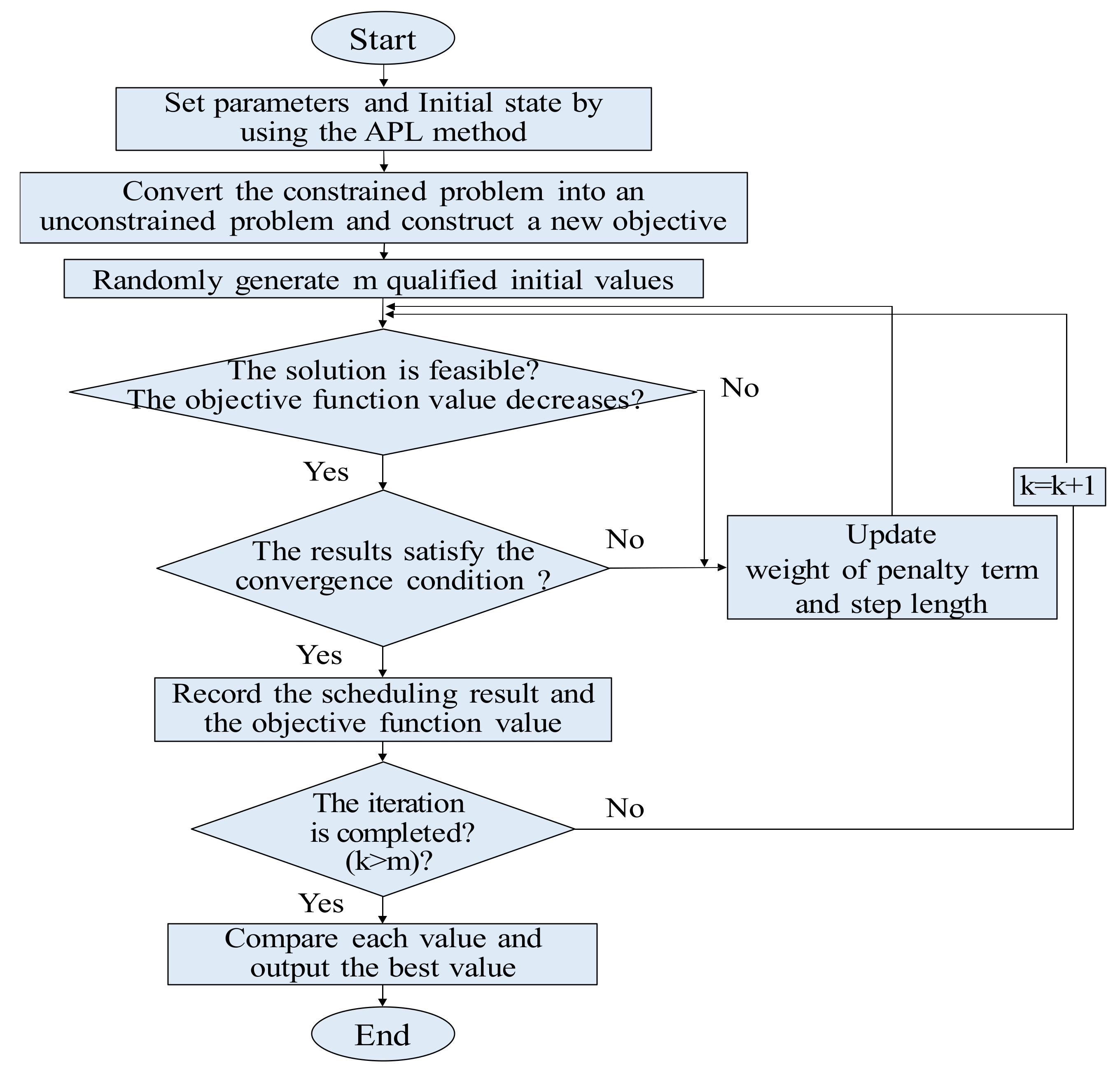
24]. The search starts from a feasible search point and proceeds along a feasible descent direction, thereby obtaining a new feasible point that causes the value of the objective function to decrease but remain within the feasible region. The flowchart of the proposed method is illustrated in
Figure 1; the steps are delineated as follows:
Step 1: Set unit parameters, initial state, and the unit selected using the APL method
Step 2: Convert the constrained problem into an unconstrained problem that has a penalty term and multiplier, and subsequently construct a new objective function called the multiplier penalty function, as shown in Equation (14). The objective function of the original problem is the first term
, the inequality (
) becomes the second term after conversion, and the equalities (
) are the third and fourth terms.
Step 3: Randomly generate m initial values (m > 0) of variables that satisfy the constraints and remain within the feasible domain, as shown in Equation (15). Let k = 0; k is the iterative value, which is compared with m to determine whether the calculation terminates
is a random sequence of numbers randomly distributed within the interval of (0,1)
Step 4: Use Equation (16) to obtain the n-dimensional optimal unit vector for the random feasible directions algorithm.
is a random value generated within the interval of (−1,1)
e is the dimension of the problem
j is the number of random directions
Step 5: Increase the number of iterations at certain proportions to obtain the step length α, as shown in Equation (17).
τ is Acceleration factor for step length
α is Particle iterative equation, presented as Equation (18)
Step 6: Use the objective function obtained at Step 2 for calculation and determine whether the solution is located within the feasible domain and whether the value of the objective function decreases. If yes, proceed to Step 7 to determine whether the convergence occurs. If no, update the weight of the penalty term
and the step length
, as presented in Equations (19) and (20).
Step 7: Determine whether the results satisfy the convergence condition
, shown in Equation (21). If yes, record the scheduling result and the objective function value; if no, update the weight of penalty term and the step length and return to Step 6.
Step 8: Finally, examine whether the iteration is completed (k > m). If yes, compare the recorded multiplier penalty function values and output the minimum total fuel cost. If no, add 1 to k and return to Step 4.
4. Simulation Results
This study used the data of 20 actual units provided by the Taiwan Power Company. The proposed HA was integrated with the APL method to fill the power gap caused by changes in the provision of renewable energy in different time periods. This study designed four scenarios: Supplementing 1560 and 1720 MW within 30 min and supplementing 1560 and 1720 MW within 10 min. To verify the advantages of the proposed method, HA was compared with IPSO and SA under the PL and APL methods.
The computer used in this study had an Intel Core i5-6400CPU@2.70GHz, 64 bits, and 16 GB of memory, and the program was written in MATLAB (MATLAB R2018, MathWorks, Natick, MA, USA).
4.1. Parameters of Taipower Units
Thermal power generating units are primarily divided into three types: Coal, heavy oil, and natural gas. Coal-fired and heavy oil-fired units are base-load units. This study employed 20 natural gas combined-cycle units provided by the Taiwan Power Company as the units for scheduling.
Table 1 presents the fuel cost parameters of various units, as well as the initial and maximum output power.
Table 2 displays the initial parameter settings for the proposed algorithm and the other two algorithms.
4.2. Unit Selection Results Using the APL Method
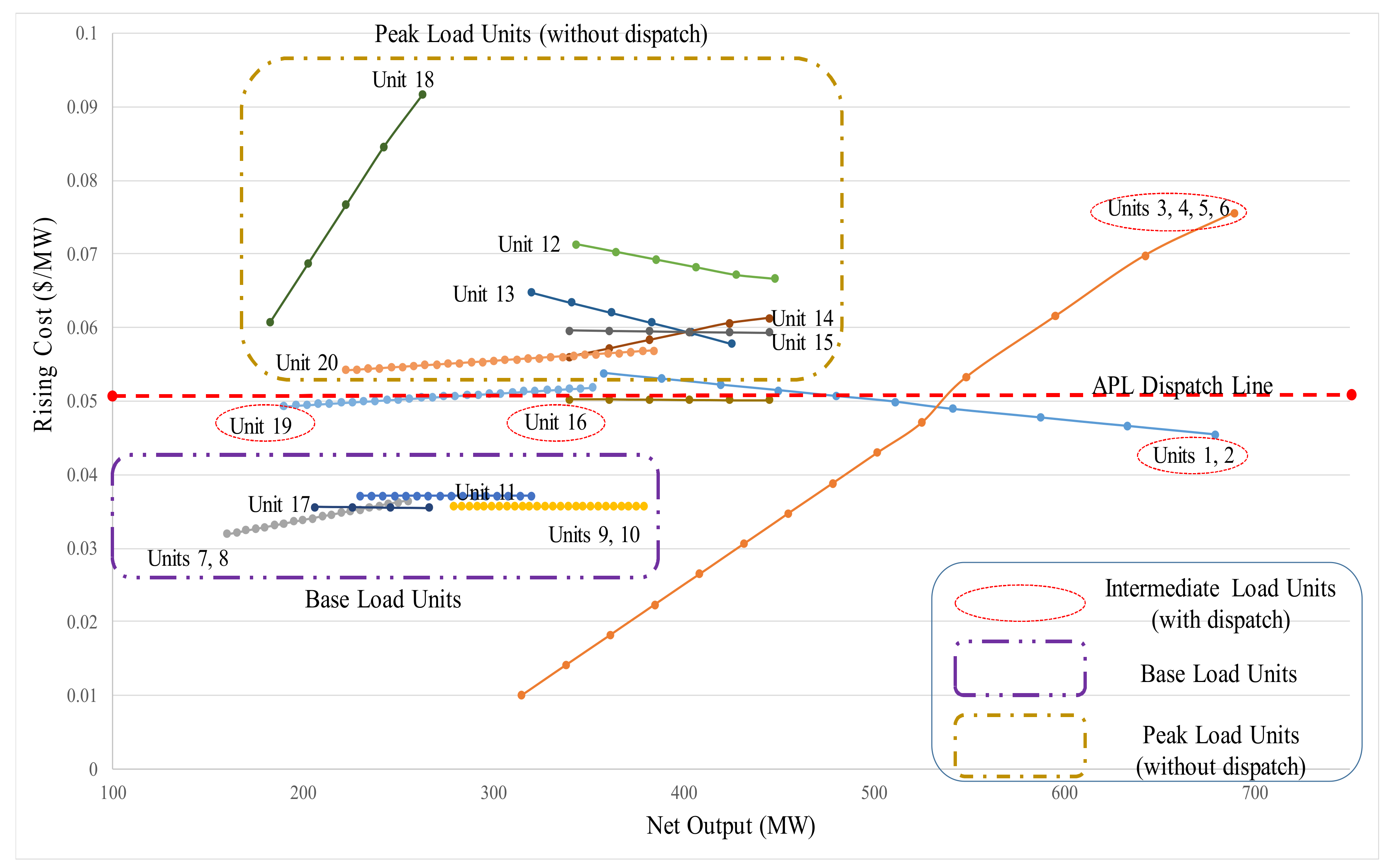
Equation (13) indicates that the ramp-up time of UC is influenced by parameter γ. The APL method was used to calculate the ramp-up cost
(y-axis) and net output (x-axis); a low y-axis value denotes a low cost (
Figure 2). To fill in a power gap of 1720 MW of renewable energy, the APL method was used to determine the units included below the area marked with red lines, namely U1–11, U16–U17, and U19; within 10 min the output power can reach 2000 MW. The dispatching principles are as follows: Units that are below the red line (no contact with the red line) are base-load units, and those that are above the red line (no contact with the red line) are peak-load units. Units that are in contact with the red line are the units requiring scheduling. Consequently, the APL method selected six peak-load units and six base-load units that were not involved in the dispatch, and eight intermediate-load units that were involved in the dispatch.
Base-load units: Units 7, 8, 9, 10, 11, 17
Peak-load units (without dispatch): Units 12, 13, 14, 15, 18, 20
Intermediate-load units (with dispatch): Units1, 2, 3, 4, 5, 6, 16, 19
4.3. Ramp-Up Scheduling Result of the Units within 30 min after the Economic Consideration
Table 3,
Table 4 and
Table 5 present the UC results generated using the proposed algorithm, IPSO, and SA after the units had been selected using the APL method. The units should generate 1560 MW of power within 30 min. The rising power is defined as the incremental amount of baseload units and dispatch units at each time period (one- or five-minute). According to
Table 3, a total of 12 units participated in the scheduling and generated 1561 MW of power, with a total cost of NT
$ 40087 and computation time of 1.56 s.
Table 4 shows the IPSO analysis results. A total of 13 units participated in the scheduling and generated 1561 MW of power, with a total cost of NT
$ 40265 and computation time of 3.84 s.
Table 5 shows the results obtained using SA. A total of 13 units participated in the scheduling and generated 1567 MW of power, with a total cost of NT
$ 40359 and computation time of 4.45 s.
The results indicated that the proposed algorithm resulted in less computation time and required fewer units being started up and a lower scheduling cost. Thus, it was superior to the other two algorithms. The SA incurred the highest cost and required the most computation time.
The comparison of the results of three algorithms in different renewable energy gap and time scenarios is shown in the
Table 6. To verify the advantages of the proposed algorithm, three scenarios were used: 1720 MW power gap of renewable energy to be filled within 30 min, and 1560 and 1720 MW within 10 min. In these scenarios, HA also exhibited the highest performance (the detailed UC results to increase power output by 1560 MW within 10 min, shown in
Table 7), followed by IPSO, and SA exhibited the lowest performance. Under the same scenario with the same three algorithms, when the PL method was used, HA still had higher performance than IPSO and SA did. This result indicated that fuel cost was lower in the ramp-up situation with a longer time (30 min) than in the emergency ramp-up situation with only a short time (10 min).
5. Conclusions
Renewable energy is expected to account for a high proportion of power generation in the future. In response to sharp decreases of renewable energy output that result in power shortages, appropriate UC problems can be solved to fill short-term power gaps.
To fill renewable energy gaps of 1720 and 1560 MW within 30 and 10 min, this study used MATLAB to write an algorithm. However, a large number of units may increase the complexity of the scheduling problem, leading to the curse of dimensionality and a failure to generate the optimal solution. This study proposed combining HA and APL to perform scheduling on 20 natural gas combined-cycle units, and the results were compared with those generated using IPSO and SA. This study found that the proposed method was superior to the other two algorithms in terms of the computation time and cost. Not only can this method precisely satisfy the constraints of the power system, but it can produce the lowest ramp-up cost. This study proposed a method that can increase system power within a specific time period through an optimal UC. Renewable energy may account for a large proportion of power generation in the future, even though renewable energy systems may have variable power output. Therefore, when a power shortage occurs due to a sudden drop in renewable energy output, the proposed method can be used for the scheduling and dispatch of power generating units. Power companies can use this method to dispatch units and governments can use these findings for promoting and implementing renewable energy power generation.


