Robust Optimization Model for Energy Purchase and Sale of Electric–Gas Interconnection System in Multi-Energy Market

Abstract

With the increasing coupling of the power system and the natural gas system, the electric–gas interconnection system has become a typical form of comprehensive energy utilization. Through the energy conversion function of the coupling unit, the system can flexibly participate in the bidding for purchasing and selling energy in a power market and a natural gas market on the premise of meeting the internal demand of multiple loads. To solve the internal coordination and optimization problem and the external flexible bidding problem in the multi-energy market, this paper proposes a robust optimization model of energy purchase and sale for the electric–gas interconnection system in a multi-energy market. Firstly, the basic structure of the electric–gas interconnection system is introduced, and the steady-state model of energy flow in the system is built based on the energy hub model. Secondly, considering the uncertainty of energy prices and the output power of renewable energy units in the system, a bidding model for energy purchase and sale of the electric–gas interconnection system in multi-energy market based on the idea of robust optimization is constructed in the framework of the Nordic energy market. Finally, empirical analysis based on the actual data is carried out, and the results prove the validity and superiority of the model. In this paper, aiming at the uncertainty of energy price, a large number of scenes are generated by Latin hypercube sampling (LHS), and then a k-means algorithm is used to reduce the scenes, so as to simulate typical scenes. Aiming at the uncertainty of the output power of the renewable energy unit in the system, a cardinal uncertainty set is used to control deviation between the actual output power and predicted output power, so that the overall robustness of the model can be controlled. The proposed model can make decision-making independent of the accurate probability distribution of uncertainty factors, and is suitable for complex multi energy systems. Meanwhile, the model possesses excellent robustness, which can effectively reduce the risk of bidding loss in the process of energy purchase and sale.

1. Introduction

An integrated energy system deepens the coupling of the power system and other energy systems by utilizing energy conversion technology, thereby integrating multiple heterogeneous energy sources to achieve multi-energy complementarity and energy cascade utilization [1,2,3]. The participation of multiple energy sources makes an integrated energy system extremely flexible in participating in market transactions [4,5]. However, due to the differences in output power characteristics, market structure, price mechanism and price volatility of heterogeneous energy sources, the decision-makers’ bidding decisions should not only consider the internal influences of output power characteristics and the coupling situation of multi-type heterogeneous energy sources, but also consider the external influence of the multi-dimensional market structure and the multi-level price system, which will bring enormous challenges for bidding decision-makers [6]. Therefore, it is urgent to carry out research on the bidding strategy of the integrated energy system in a multi-energy market, which will provide a scientific and reasonable decision-making basis for both the internal multi-energy collaborative operation management and the external multi energy market bidding.

The electric–gas interconnection system, mostly based on industrial parks, is an integrated energy system with broad development prospects [7,8]. The system is connected with a public power network and natural gas pipeline network externally, and can realize combined gas-heating-cooling-power supply through an energy conversion unit internally, whose internal energy conversion and utilization are relatively independent [9,10]. Considering that the electric–gas interconnection system involves the coupling and conversion of gas-heating-cooling-power energy sources, it is necessary to build the steady-state model of energy flow about multi-type heterogeneous energy in decision-making optimization [11,12,13,14]. An energy hub model is widely used in energy flow analysis of the multi-energy systems, especially in the research about planning and operation optimization of multi-energy systems, which is defined as an input–output port model for describing the exchange and coupling relationship of energy, load and network under the multi-energy systems. So far, however, the general energy hub models seldom consider the influence of system uncertainties, which greatly reduce the practical application effect of the model.

In the interaction process with the external multi-energy market, the role of the electric–gas interconnection system is not only the energy producer, but also the energy consumer [15]. When its internal energy supply cannot meet demand, it will purchase energy from the external natural gas market or the power market, and when its internal energy supply exceeds the demand, it can sell the surplus to the natural gas market or the power market. The particularity of its positioning makes its bidding behavior different from that of the traditional generation side or the user side market [11,12,13,14,15]. Meanwhile, due to the fact that the electric–gas interconnection system can flexibly participate in the purchase and sale of energy in the multi-energy system, it is necessary to make a coordinated bidding decision in the multi-energy market. So far, there have been many research works on the bidding strategy optimization for both generation side or user side in the power system, and the bidding decision-making subjects mainly include single energy generator, joint generator of renewable energy and traditional energy, joint generator of renewable energy and energy conversion unit, virtual power plant considering demand side resources, electricity seller of multi-type load aggregation, large consumer, micro-grid subject of paralleling in the network or off-network flexibly, etc.. All the bidding decision-making subjects except the micro-grid only participate in market transactions as a single buyer or a single seller. Due to the limitations of the decision-making subjects and market background, there are few studies on the optimization of energy bidding decision-making which consider the duality of the multi energy system’s identity in the market and the differences of the multi energy market.

When research into the bidding decision-making optimization method is carried out, according to the treatment of uncertain variables, optimization methods can be generally divided into two categories: stochastic optimization and robust optimization [16]. Stochastic optimization, depending on the probability distribution of uncertain variables, can transform uncertain optimization problems into deterministic optimization problems by describing the continuous or discrete probability distribution characteristics of uncertain variables. However, there are many problems in this method, such as the fact that it easily falls into dimension disaster, a high accuracy requirement for probability estimation, poor anti-noise ability and so on. Robust optimization is an optimization method that considers the influence of the worst-case on system decision-making. Compared with stochastic optimization, robust optimization focuses on the boundary condition of uncertain variables, so it is not necessary to obtain the accurate probability distribution of uncertain variables, and its conservatism can be controlled by adjusting the scale of uncertainty set [17]. A robust optimization method can effectively solve the problems such as high sensitivity of the model to the parameters and large influence of parameter estimation error on the model, which is widely used in the power system unit commitment [18] and economic dispatch [19,20,21], but seldom used in the multi-energy system.

Based on the above background, this paper proposes a robust optimization model of energy purchase and sale for the electric–gas interconnection system in the multi-energy market. Firstly, the basic structure of the electric–gas interconnection system is introduced, and the steady-state model of energy flow in the system is built based on the energy hub model. Secondly, in the framework of Nordic energy market, a bidding model for energy purchase and sale of the electric–gas interconnection system in the multi-energy market based on the idea of robust optimization is constructed, considering the uncertainty of energy price and the output power of renewable energy units in the system. Finally, empirical analysis based on the actual data is carried out, and the results prove the validity and superiority of the model. In this paper, aiming at the uncertainty of energy prices, a large number of scenes are generated by Latin hypercube sampling (LHS), and then k-means algorithm is used to reduce the scenes, so as to simulate typical scenes. Aiming at the uncertainty of the output power of the renewable energy unit in the system, cardinal uncertainty set is used to control the deviation between the actual output power and the predicted output power, so that the overall robustness of the model can be controlled. The proposed model can make decision-making independent of the accurate probability distribution of uncertainty factors, and is suitable for complex multi-energy systems. Meanwhile, the model possesses excellent robustness, which can effectively reduce the risk of bidding loss in the process of energy purchase and sale.

2. Steady-State Model of Energy Flow in the Electric–Gas Interconnection System

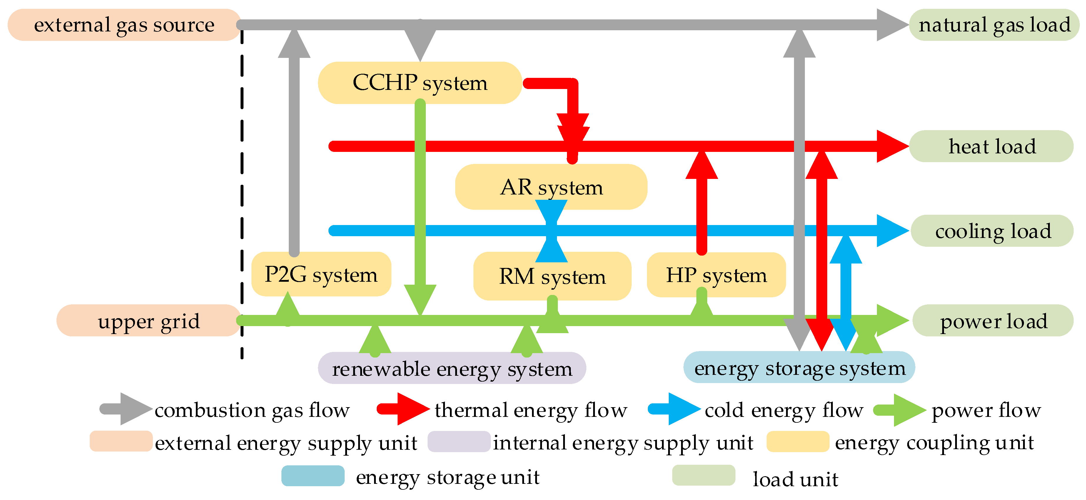
2.1. Typical Structure of the Electric–Gas Interconnection System

The electric–gas interconnection system consists of the natural gas system, the heating system, the cooling system and the power system distributed in the same area. The system components can be divided into external energy supply unit, internal energy supply unit, energy coupling unit, energy storage unit, energy supply network and load unit. The typical structure of the electric–gas interconnection system is shown in Figure 1, and the return water network for cooling and heating is not shown in this figure.

Power load in the power system is supplied by the distributed or cluster renewable energy system (RES), the combined heat and power (CHP) system, the energy storage (ES) system and the upper grid. Heat load in the heating system is supplied by the CHP system, the heat pump (HP) system and the heat storage system [22]. Cooling load in the cooling system is transformed and supplied by the absorption refrigeration (AR) system, the refrigerating machine (RM) system and the cooling storage system. Natural gas load in the gas supply system is supplied by the power-to-gas (P2G) system, external gas sources and gas storage tank. The natural gas pipeline network, as the low-pressure gas distribution network (7.5 × 103pa and below), is usually equipped with a pressure regulating device at the air sources, without considering the compressor and pressure regulating equipment temporarily. In conclusion, due to the introduction of a series of coupling elements, the system enhances the strong multi energy coupling relationship, which requires joint analysis.

2.2. Energy Hub Model of Energy Flow in the Electric–Gas Interconnection System

The establishment of steady-state model of energy flow of multi-type heterogeneous energy in the electric–gas interconnection system is the basic premise for decision-makers to make decision optimization. The energy hub model is widely used in the steady-state modeling of energy flow [14,16]. In this model, for an energy conversion device with only single input and single output, the relationship between input and output is as follows:

$$L_{\alpha }={\eta }_{\alpha , \beta }{P}_{\beta }$$

(1)

where, $L_{\alpha }$ and $P_{\beta }$ are the input and output of the steady-state system; ${\eta }_{\alpha ,\beta }$ is the coupling coefficient between the input and output.

The integrated energy system consists of multiple energy conversion devices and various energy forms. The coupling relationship between input and output in the system can be described by the energy hub model. The formula is as follows:

$$\underset{L}{\left[\begin{array}{c}{L}_{\alpha }\\ L_{\beta }\\ ⋮\\ L_{\omega }\end{array}\right]}=\underset{\eta }{\left[\begin{array}{cccc}{\eta }_{\alpha \alpha }& {\eta }_{\beta \alpha }& \cdots & {\eta }_{\omega \alpha }\\ {\eta }_{\alpha \beta }& {\eta }_{\beta \beta }& \cdots & {\eta }_{\omega \beta }\\ ⋮& ⋮& ⋮& ⋮\\ {\eta }_{\alpha \omega }& {\eta }_{\beta \omega }& \cdots & {\eta }_{\omega \omega }\end{array}\right]}\underset{P}{\left[\begin{array}{c}{P}_{\alpha }\\ P_{\beta }\\ ⋮\\ P_{\omega }\end{array}\right]}$$

(2)

where, vectors $P$ and $L$ are the input and output variables of the system respectively. Each coupling coefficient in the coupling matrix $\eta$ corresponds to the coupling relationship between a specific input and a specific output.

By combining the energy concentrator conversion matrix and the flow direction of different energy sources in the electric–gas interconnection system shown in Figure 1, the corresponding energy input and output relations of natural gas, heat, cooling and the power systems in the electric–gas interconnection system can be obtained. Due to the bidding period $t=1h$, the power and energy (electric quantity and natural gas quantity) of each bidding period are the same in numerical value. Without specification, the bidding power (Unit: MW) is adopted below to describe the model. The energy conversion model of the natural gas system is as follows:

$$L_{\mathrm{G},t}=-P_{\mathrm{G},t}^{\mathrm{bid}}+{\eta }^{\mathrm{P}2\mathrm{G}}{P}_{\mathrm{E},t}^{\mathrm{P}2\mathrm{G}}-P_{\mathrm{G},t}^{\mathrm{CHP}}-P_{\mathrm{G},t}^{\mathrm{ch}\arg \mathrm{e}}+P_{\mathrm{G},t}^{\mathrm{disch}\arg \mathrm{e}}$$

(3)

where, $L_{\mathrm{G},t}$(Unit: MW) represents the output power of the natural gas system in the $t$ period, and subscript $t$ represents the time scale variable, the same below. $P_{\mathrm{G},t}^{\mathrm{bid}}$(Unit: MW) represents the natural gas power purchased or sold, which is positive when sold and negative when purchased. ${\eta }^{\mathrm{P}2\mathrm{G}}$(Unit: %) represents the conversion efficiency of electricity to gas. $P_{\mathrm{E},t}^{\mathrm{P}2\mathrm{G}}$(Unit: MW) represents the power allocated by the power system to the P2G system. $P_{\mathrm{G},t}^{\mathrm{CHP}}$(Unit: MW) represents the power allocated by the natural gas system to the CHP system. $P_{\mathrm{G},t}^{\mathrm{ch}\arg \mathrm{e}}$(Unit: MW) represents the air charge power of the air tank. $P_{\mathrm{G},t}^{\mathrm{disch}\arg \mathrm{e}}$(Unit: MW) represents the air discharge power of the air tank.

The energy conversion model of the heating system in the electric–gas interconnection system is as follows:

$$L_{\mathrm{H},t}={\eta }_{\mathrm{H}}^{\mathrm{CHP}}{P}_{\mathrm{G},t}^{\mathrm{CHP}}-P_{\mathrm{H},t}^{\mathrm{AR}}+{\eta }^{\mathrm{HP}}{P}_{\mathrm{E},t}^{\mathrm{HP}}$$

(4)

where, $L_{\mathrm{H},t}$(Unit: MW) represents the output power of the heating system. ${\eta }_{\mathrm{H}}^{\mathrm{CHP}}$(Unit: %) represents the heating efficiency of CHP. $P_{\mathrm{H},t}^{\mathrm{AR}}$(Unit: MW) represents the power allocated by the heating system to the AR system. ${\eta }^{\mathrm{HP}}$(Unit: %) represents the heating efficiency of the heat pump. $P_{\mathrm{E},t}^{\mathrm{HP}}$(Unit: MW) represents the power allocated by the power system to the HP system.

The energy conversion model of the cooling system is as follows:

$$L_{\mathrm{C},t}={\eta }^{\mathrm{AR}}{P}_{\mathrm{H},t}^{\mathrm{AR}}+{\eta }^{\mathrm{RM}}{P}_{\mathrm{E},t}^{\mathrm{RM}}$$

(5)

where, $L_{\mathrm{C},t}$(Unit: MW) represents the output power of the cooling system, ${\eta }^{\mathrm{AR}}$(Unit: %) represents the cooling efficiency of the AR system, ${\eta }^{\mathrm{RM}}$(Unit: %) represents the cooling efficiency of the RM system, and $P_{\mathrm{E},t}^{\mathrm{RM}}$(Unit: MW) represents the power allocated by the power system to the RM system.

The energy conversion model of the power supply system is as follows:

$$L_{\mathrm{E},t}=-\widetilde{P_{\mathrm{E},t}^{\mathrm{real}}}+P_{\mathrm{E},t}^{\mathrm{RES}}+{\eta }_{\mathrm{E}}^{\mathrm{CHP}}{P}_{\mathrm{G},t}^{\mathrm{CHP}}-P_{\mathrm{E},t}^{\mathrm{P}2\mathrm{G}}-P_{\mathrm{E},t}^{\mathrm{RM}}-P_{\mathrm{E},t}^{\mathrm{HP}}-P_{\mathrm{E},t}^{\mathrm{ch}\arg \mathrm{e}}+P_{\mathrm{E},t}^{\mathrm{disch}\arg \mathrm{e}}$$

(6)

where, $L_{\mathrm{G},t}$ represents the output power of the power system. $\widetilde{P_{\mathrm{E},t}^{\mathrm{real}}}$ represents the predicted value of the actual power purchased or sold, which is positive when sold and negative when purchased. $P_{\mathrm{E},t}^{\mathrm{RES}}$ represents the output power of the RE system. $P_{\mathrm{E},t}^{\mathrm{ch}\arg \mathrm{e}}$ represents the energy storage power of the ES system, and $P_{\mathrm{E},t}^{\mathrm{disch}\arg \mathrm{e}}$ represents the discharge power of the ES system.

2.3. Dynamic Energy Charging and Discharging Model of the Energy Storage (ES) System

Energy storage equipment is an important equipment of energy hub, which can transfer energy in a time dimension. Excess energy or cheap energy can be stored by energy storage equipment and released when the energy demand is large or the energy price is high, which can make efficient use of energy and reduce energy cost.

In a broad sense, energy storage includes not only electricity storage (battery), but also heat storage (the hot water storage system), gas storage (gas storage tank), cooling storage (ice storage, water storage, etc.). Their processes of energy charging and discharging are similar, which need to consider the constraints of multiple periods, mainly including the constraints of charging and discharging state, energy storage and so on. The general dynamic model of generalized energy storage can be expressed as follows:

$$u_t^{\mathrm{ch}\arg \mathrm{e}}+u_t^{\mathrm{disch}\arg \mathrm{e}}\le 1$$

(7)

$$u_t^{\mathrm{ch}\arg \mathrm{e}}{P}_{\min }^{\mathrm{ch}\arg \mathrm{e}}\le P_t^{\mathrm{ch}\arg \mathrm{e}}\le u_t^{\mathrm{ch}\arg \mathrm{e}}{P}_{\max }^{\mathrm{ch}\arg \mathrm{e}}$$

(8)

$$u_t^{\mathrm{disch}\arg \mathrm{e}}{P}_{\min }^{\mathrm{disch}\arg \mathrm{e}}\le P_t^{\mathrm{disch}\arg \mathrm{e}}\le u_t^{\mathrm{disch}\arg \mathrm{e}}{P}_{\max }^{\mathrm{disch}\arg \mathrm{e}}$$

(9)

$$Q_{t+1}^{\mathrm{storage}}=Q_t^{\mathrm{storage}}(1-{\delta }^{\mathrm{storage}})+({\eta }_{}^{\mathrm{ch}\arg \mathrm{e}}{P}_t^{\mathrm{ch}\arg \mathrm{e}}-\frac{P_t^{\mathrm{disch}\arg \mathrm{e}}}{{\eta }_{}^{\mathrm{disch}\arg \mathrm{e}}})\Delta t$$

(10)

$$Q_{\min }^{\mathrm{storage}}\le Q_t^{\mathrm{storage}}\le Q_{\max }^{\mathrm{storage}}$$

(11)

$$Q_{24}^{\mathrm{storage}}=Q_0^{\mathrm{storage}}$$

(12)

where, $u_t^{\mathrm{ch}\arg \mathrm{e}}$ and $u_t^{\mathrm{disch}\arg \mathrm{e}}$ represent the charging and discharging states of energy storage equipment respectively, which are 0–1 variables. 1 represents the working state, and 0 represents the non-working state. Equation (7) shows the limit of charging and discharging energy of energy storage equipment. $P_{\max }^{\mathrm{ch}\arg \mathrm{e}}$(Unit: MW), $P_{\min }^{\mathrm{ch}\arg \mathrm{e}}$(Unit: MW), $P_{\max }^{\mathrm{disch}\arg \mathrm{e}}$(Unit: MW) and $P_{\min }^{\mathrm{disch}\arg \mathrm{e}}$(Unit: MW) represent the upper and lower limits of the charging and discharging energy of the ES system respectively. Equation (10) shows the energy change before and after charging and discharging of the ES system. $Q_{t+1}^{\mathrm{storage}}$(Unit: MWh) and $Q_t^{\mathrm{storage}}$(Unit: MWh) represent the energy storage of the ES system in the $t+1$ and $t$ period respectively. ${\eta }_{\mathrm{E}}^{\mathrm{ch}\arg \mathrm{e}}$(Unit: %) and ${\eta }_{\mathrm{E}}^{\mathrm{disch}\arg \mathrm{e}}$ represent charge efficiency and discharge efficiency of the ES system respectively. $Q_{\max }^{\mathrm{storage}}$(Unit: MWh) and $Q_{\min }^{\mathrm{storage}}$(Unit: MWh) represent upper and lower limits of the energy storage in the ES system respectively. Equation (12) shows that the energy storage of the energy storage equipment is equal at the end time and the initial time.

3. Optimization Model for Energy Purchase and Sale of the Electric–Gas Interconnection System

3.1. Market Structure and Bidding Process

Assuming that the electric–gas interconnection system is the price acceptor in both the power market and the natural gas market, the decision maker of the system only needs to optimize his bidding volume according to the predicted market transaction price when bidding. In the day-ahead power market and the day-ahead natural gas market, the bidding is conducted in hours, that is, there are 24 bidding periods in each trading day, and the decision maker of the system can choose to declare as the buyer or the seller in each period.

Considering the relative maturity of the Nordic power market, the research work of this paper is based on the simplified market mechanism of Nord pool. The bidding process of the Nordic power market is shown in Figure 2:

The bidding process of the Nordic power market is as follows: the day-ahead market on the $Dth$ day will be closed at 12:00 pm on the $(D-1)th$ day, and all participants need to submit the bidding information (combination of price and electric quantity) of $T$ ($T$ = 24) trading periods on the $Dth$ day to the dispatching authority before that.

The time interval from the close of the day-ahead market to the start of the real-time dispatching on the $Dth$ day is long, and the predicted power supply and demand situation will generally deviate from the actual situation. The system dispatching operation organization can balance the supply and demand deviation through the intra-day market, and carry out unbalanced electric quantity settlement after the end of the day’s operation.

The generation of renewable energy in the electric–gas interconnection system is uncontrollable, and the bidding subject of the electric–gas interconnection system may use the price difference between the power market and the natural gas market for arbitrage, so the actual output power of the electric–gas interconnection system in the next day may deviate from the declared value of the previous output power. The independent dispatching organization needs to mobilize other adjustable units to balance the output power deviation, resulting in the re-dispatching cost of the system. In the Nordic power market, although the pricing mechanism of unbalanced electric quantity in different countries is slightly different, its formulation principle is to ensure that the income of unbalanced electric quantity is lower than the trading income in the day-ahead market or in the intra-day market. Therefore, this paper charges the unbalanced electric quantity with the penalty price.

The Nordic natural gas trading market mainly includes within day contracts market, day contracts market and month contracts market. The natural gas buyer or seller submits the purchased or sold quantities and prices of natural gas to the natural gas trading hub, and the trading system automatically matches the order according to the bid of the buyer and the seller. At the end of the day, the trading system calculates the average trading price of the day by weighting according to the quantities and prices of natural gas on that day. This paper discusses the bidding strategy of the electric–gas interconnection system in the power market and the natural gas market. Since the transaction price of natural gas cannot be determined before the transaction actually occurs, and the fluctuation of the natural gas clearing price is small, the average transaction price of natural gas is taken as the price of natural gas purchase or sale approximately.

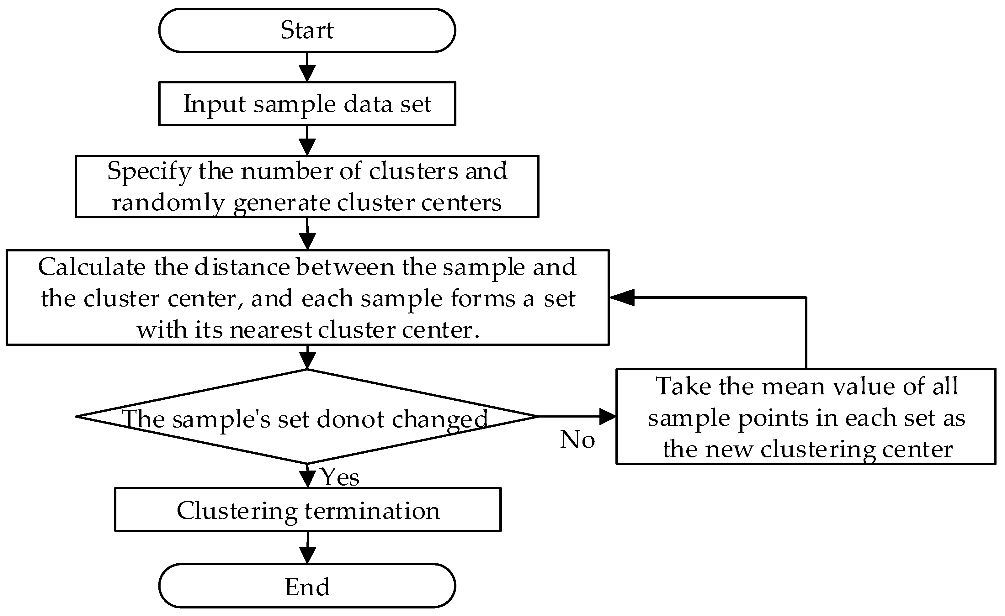
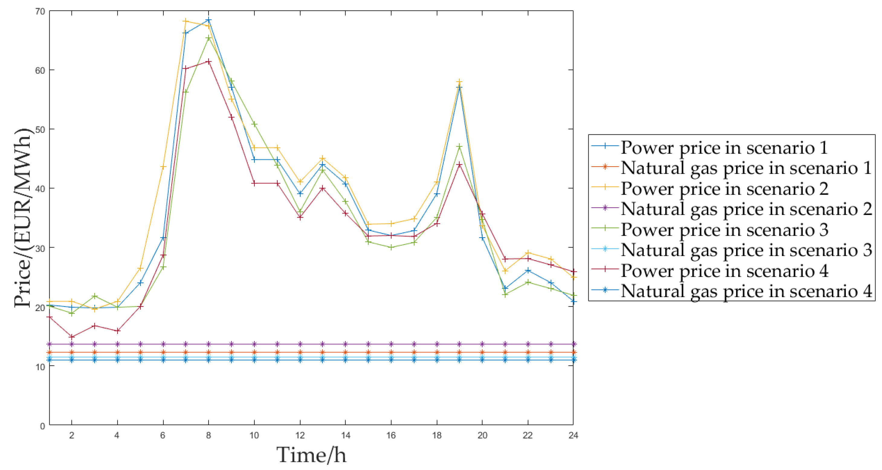
3.2. Treatment of Uncertain Factors

When the electric–gas interconnection system participates in the bidding of the multi-energy market, the uncertain variables involved include the clearing price of the power market, the average clearing price of the natural gas market, the penalty price of unbalanced electric quantity, and the actual output power of the system in the next day. Two kinds of uncertain variables, price and output power, are dealt with by the scenario analysis method and cardinal uncertainty set method respectively.

The clearing price of the power market, the clearing price of the natural gas market, and the penalty price of unbalanced electricity quantity will directly affect the income of the electric–gas interconnection system, while the clearing price is affected by the bidding behavior of the market subjects, load fluctuation and other factors, which has considerable volatility and uncertainty. When using the scenario analysis method to describe the uncertainty of these factors, it can deal with uncertainty factors and carry out risk analysis by calculating the maximum (or minimum) expectation of the model objective function in various scenarios.

First of all, according to the historical data of clearing price in the power market and the natural gas market, a specific probability distribution can be obtained by data fitting. Then, a large number of scenes are obtained by sampling. The larger the number of scenes are, the more accurate the results are, but the larger the calculation amount is. In order to balance the calculation amount and accuracy, firstly, according to the probability distribution of market clearing price, a large number of scenarios are generated by Latin hypercube sampling (LHS). Then, the k-means algorithm is used to reduce and merge the scene, and the probability of the scene after merging is calculated. The flow of the k-means algorithm is shown in the Figure 3.

For the uncertainty of the next day’s actual output power of the electric–gas interconnection system, select the appropriate ‘uncertainty set’ to be expressed. At present, the uncertain sets are often described in the form of box type, polyhedron type, ellipsoid type, cardinal type, etc. The characteristic of the cardinal uncertainty set used in this paper is that it can control the relative value of the uncertainty parameter offset and measure the parameter fluctuation accurately. The cardinal uncertainty set of the next day’s actual output power of the electric–gas interconnection system is expressed as follows:

$$\Omega =\{\widetilde{P_{\mathrm{E},t}^{\mathrm{real}}}:P_{\mathrm{E},t,k}^{\mathrm{real},\min }\le \widetilde{P_{\mathrm{E},t}^{\mathrm{real}}}\le P_{\mathrm{E},t,k}^{\mathrm{real},\max },\begin{array}{cc}& {\displaystyle \sum _{t=1}^T\left|\frac{\widetilde{P_{\mathrm{E},t}^{\mathrm{real}}}-\stackrel{\wedge }{P_{\mathrm{E},t}^{\mathrm{real}}}}{\stackrel{\Delta }{P_{\mathrm{E},t}^{\mathrm{real}}}}\right|\le \Gamma \}}\end{array}$$

(13)

where, $\Omega$ represents the uncertainty set of the next day’s actual output power of the electric–gas interconnection system. $P_{\mathrm{E},t,k}^{\mathrm{real},\max }$(Unit: MW) and $P_{\mathrm{E},t,k}^{\mathrm{real},\min }$(Unit: MW) represent the upper and lower limits of the next day’s actual output power of the electric–gas interconnection system respectively. $\stackrel{\wedge }{P_{\mathrm{E},t}^{\mathrm{real}}}$(Unit: MW) is the midpoint of the confidence interval of the next day’s actual output power. $\stackrel{\Delta }{P_{\mathrm{E},t}^{\mathrm{real}}}$(Unit: MW) represents the maximum deviation.

3.3. Robust Model for Energy Purchase and Sale of the Electric–Gas Interconnection System

The model assumes that:

(1)

Both the power market and the natural gas market involved in the transaction are bilateral markets, and energy can be purchased or sold flexibly.

(2)

The scale of the electric–gas interconnection system is not enough to influence the power market and the natural gas market.

(3)

The positive deviation and negative deviation of the actual intra-day purchase or sale of electric quantity of the electric–gas interconnection system use the same penalty price to settle the unbalanced electric quantity.

(4)

In the natural gas market, the price is relatively stable and there is no deviation penalty mechanism.

Robust optimization is an optimization method that makes a decision based on the uncertainty of influencing factors. Its goal is to get the optimal decision under the worst case of uncertain factors. Therefore, when using robust optimization for decision-making, it is necessary to make clear what the worst impact of uncertain factors on profits is. Although the worst situation may not occur in reality, it is still necessary to consider and make decisions based on the worst case, so as to avoid the serious consequences brought by the worst-case as much as possible. Therefore, this paper establishes the purchase and sale decision-making model of the electric–gas interconnection system as follows

$$\underset{P_{\mathrm{E},t}^{\mathrm{bid}},P_{\mathrm{G},t}^{\mathrm{bid}}}{\max }\underset{\widetilde{P_{\mathrm{E},t}^{\mathrm{real}}}}{\min }\mathrm{E}{\displaystyle \sum _{t=1}^T[{\lambda }_{\mathrm{E},t}{P}_{\mathrm{E},t}^{\mathrm{bid}}+{\lambda }_{\mathrm{G},t}{P}_{\mathrm{G},t}^{\mathrm{bid}}-{\lambda }_{\mathrm{R},t}({\Delta }_{\mathrm{E},t}^{+}+{\Delta }_{\mathrm{E},t}^{-})]}$$

(14)

$${\Delta }_{\mathrm{E},t}^{+}=\max \{\widetilde{P_{\mathrm{E},t}^{\mathrm{real}}}-P_{\mathrm{E},t}^{\mathrm{bid}},0\}$$

(15)

$${\Delta }_{\mathrm{E},t}^{-}=\max \{P_{\mathrm{E},t}^{\mathrm{bid}}-\widetilde{P_{\mathrm{E},t}^{\mathrm{real}}},0\}$$

(16)

$$\widetilde{P_{\mathrm{E},t}^{\mathrm{real}}}\in \Omega$$

(17)

$$P_{\mathrm{E},t}^{\mathrm{bid},\min }\le P_{\mathrm{E},t}^{\mathrm{bid}}\le P_{\mathrm{E},t}^{\mathrm{bid},\max }$$

(18)

$$P_{\mathrm{G},t}^{\mathrm{bid},\min }\le P_{\mathrm{G},t}^{\mathrm{bid}}\le P_{\mathrm{G},t}^{\mathrm{bid},\max }$$

(19)

$$P_{\mathrm{E},t}^{\mathrm{RES},\min }\le P_{\mathrm{E},t}^{\mathrm{RES}}\le P_{\mathrm{E},t}^{\mathrm{RES},\max }$$

(20)

$$P_{\mathrm{G}}^{\mathrm{P}2\mathrm{G},\min }\le {\eta }^{\mathrm{P}2\mathrm{G}}{P}_{\mathrm{E},t}^{\mathrm{P}2\mathrm{G}}\le P_{\mathrm{G}}^{\mathrm{P}2\mathrm{G},\max }$$

(21)

$$P_{\mathrm{H}}^{\mathrm{CHP},\min }\le {\eta }_{\mathrm{H}}^{\mathrm{CHP}}{P}_{\mathrm{G},t}^{\mathrm{CHP}}\le P_{\mathrm{H}}^{\mathrm{CHP},\max }$$

(22)

$$P_{\mathrm{E}}^{\mathrm{CHP},\min }\le {\eta }_{\mathrm{E}}^{\mathrm{CHP}}{P}_{\mathrm{G},t}^{\mathrm{CHP}}\le P_{\mathrm{E}}^{\mathrm{CHP},\max }$$

(23)

$$P_{\mathrm{H}}^{\mathrm{HP},\min }\le {\eta }^{\mathrm{HP}}{P}_{\mathrm{E},t}^{\mathrm{HP}}\le P_{\mathrm{H}}^{\mathrm{HP},\max }$$

(24)

$$P_{\mathrm{C}}^{\mathrm{AR},\min }\le {\eta }^{\mathrm{AR}}{P}_{\mathrm{H},t}^{\mathrm{AR}}\le P_{\mathrm{C}}^{\mathrm{AR},\max }$$

(25)

$$P_{\mathrm{C}}^{\mathrm{RM},\min }\le {\eta }^{\mathrm{RM}}{P}_{\mathrm{E},t}^{\mathrm{RM}}\le P_{\mathrm{C}}^{\mathrm{RM},\max }$$

(26)

$$L_{\mathrm{G},t}=-P_{\mathrm{G},t}^{\mathrm{bid}}+{\eta }^{\mathrm{P}2\mathrm{G}}{P}_{\mathrm{E},t}^{\mathrm{P}2\mathrm{G}}-P_{\mathrm{G},t}^{\mathrm{CHP}}-P_{\mathrm{G},t}^{\mathrm{ch}\arg \mathrm{e}}+P_{\mathrm{G},t}^{\mathrm{disch}\arg \mathrm{e}}$$

(27)

$$L_{\mathrm{H},t}={\eta }_{\mathrm{H}}^{\mathrm{CHP}}{P}_{\mathrm{G},t}^{\mathrm{CHP}}-P_{\mathrm{H},t}^{\mathrm{AR}}+{\eta }^{\mathrm{HP}}{P}_{\mathrm{E},t}^{\mathrm{HP}}$$

(28)

$$L_{\mathrm{C},t}={\eta }^{\mathrm{AR}}{P}_{\mathrm{H},t}^{\mathrm{AR}}+{\eta }^{\mathrm{RM}}{P}_{\mathrm{E},t}^{\mathrm{RM}}$$

(29)

$$L_{\mathrm{E},t}=-\widetilde{P_{\mathrm{E},t}^{\mathrm{real}}}+P_{\mathrm{E},t}^{\mathrm{RES}}+{\eta }_{\mathrm{E}}^{\mathrm{CHP}}{P}_{\mathrm{G},t}^{\mathrm{CHP}}-P_{\mathrm{E},t}^{\mathrm{P}2\mathrm{G}}-P_{\mathrm{E},t}^{\mathrm{RM}}-P_{\mathrm{E},t}^{\mathrm{HP}}-P_{\mathrm{E},t}^{\mathrm{ch}\arg \mathrm{e}}+P_{\mathrm{E},t}^{\mathrm{disch}\arg \mathrm{e}}$$

(30)

$$u_t^{\mathrm{ch}\arg \mathrm{e}}+u_t^{\mathrm{disch}\arg \mathrm{e}}\le 1$$

(31)

$$u_t^{\mathrm{ch}\arg \mathrm{e}}{P}_{\min }^{\mathrm{ch}\arg \mathrm{e}}\le P_t^{\mathrm{ch}\arg \mathrm{e}}\le u_t^{\mathrm{ch}\arg \mathrm{e}}{P}_{\max }^{\mathrm{ch}\arg \mathrm{e}}$$

(32)

$$u_t^{\mathrm{disch}\arg \mathrm{e}}{P}_{\min }^{\mathrm{disch}\arg \mathrm{e}}\le P_t^{\mathrm{disch}\arg \mathrm{e}}\le u_t^{\mathrm{disch}\arg \mathrm{e}}{P}_{\max }^{\mathrm{disch}\arg \mathrm{e}}$$

(33)

$$Q_{t+1}^{\mathrm{storage}}=Q_t^{\mathrm{storage}}(1-{\delta }^{\mathrm{storage}})+({\eta }_{}^{\mathrm{ch}\arg \mathrm{e}}{P}_t^{\mathrm{ch}\arg \mathrm{e}}-\frac{P_t^{\mathrm{disch}\arg \mathrm{e}}}{{\eta }_{}^{\mathrm{disch}\arg \mathrm{e}}})\Delta t$$

(34)

$$Q_{\min }^{\mathrm{storage}}\le Q_t^{\mathrm{storage}}\le Q_{\max }^{\mathrm{storage}}$$

(35)

$$Q_{24}^{\mathrm{storage}}=Q_0^{\mathrm{storage}}$$

(36)

where, ${\lambda }_{\mathrm{E},t}$(Unit: EUR/MW), ${\lambda }_{\mathrm{G},t}$(Unit: EUR/MW) and ${\lambda }_{\mathrm{R},t}$(Unit: EUR/MW) represent the clearing price of the day-ahead power market, the average transaction price of the natural gas market and the penalty price of unbalanced electric quantity. ${\Delta }_{\mathrm{E},t}^{+}$(Unit: MW) and ${\Delta }_{\mathrm{E},t}^{-}$(Unit: MW) represent positive deviation and negative deviation, respectively. $P_{\mathrm{E},t}^{\mathrm{bid},\max }$(Unit: MW) and $P_{\mathrm{E},t}^{\mathrm{bid},\min }$(Unit: MW) represent the upper and lower limits of bidding power in the $t$ period of the next day submitted by the system in the power market, respectively. $P_{\mathrm{G},t}^{\mathrm{bid},\max }$(Unit: MW) and $P_{\mathrm{G},t}^{\mathrm{bid},\min }$(Unit: MW) represent the upper and lower limits of bidding power in the $t$ period of the next day submitted by the system in the natural gas market, respectively. $P_{\mathrm{E},t}^{\mathrm{RES},\max }$(Unit: MW) and $P_{\mathrm{E},t}^{\mathrm{RES},\min }$(Unit: MW) represent the upper and lower limits of the output power of the RE system in the $t$ period of the next day, respectively. $P_{\mathrm{G}}^{\mathrm{P}2\mathrm{G},\max }$(Unit: MW) and $P_{\mathrm{G}}^{\mathrm{P}2\mathrm{G},\min }$(Unit: MW) represent the upper and lower limits of natural gas output power of the P2G system, respectively. $P_{\mathrm{H}}^{\mathrm{CHP},\max }$(Unit: MW) and $P_{\mathrm{H}}^{\mathrm{CHP},\min }$(Unit: MW) represent the upper and lower limits of thermal output power of the CHP system, respectively. $P_{\mathrm{H}}^{\mathrm{HP},\max }$(Unit: MW) and $P_{\mathrm{H}}^{\mathrm{HP},\min }$(Unit: MW) represent the upper and lower limits of thermal output power of the HP system, respectively. $P_{\mathrm{C}}^{\mathrm{AR},\max }$(Unit: MW) and $P_{\mathrm{C}}^{\mathrm{AR},\min }$(Unit: MW) represent the upper and lower limits of cold output power of the AR system respectively. $P_{\mathrm{C}}^{\mathrm{RM},\max }$(Unit: MW) and $P_{\mathrm{C}}^{\mathrm{RM},\min }$(Unit: MW) represent the upper and lower limits of cold output power of the RM system, respectively. Formulas (27)–(30) represent the energy balance of the electric–gas interconnection system. Formulas (31)–(36) represent the operation constraints of the energy storage equipment installed in the electric–gas interconnection system.

3.4. Model Transformation

In the process of solving the above robust optimization model, considering that some components in Formula (14) are independent of variables, Formula (14) can be simplified as follows:

$$\underset{P_{\mathrm{E},t}^{\mathrm{bid}},P_{\mathrm{G},t}^{\mathrm{bid}}}{\max }\mathrm{E}\left\{{\displaystyle \sum _{t=1}^T({\lambda }_{\mathrm{E},t}{P}_{\mathrm{E},t}^{\mathrm{bid}}+{\lambda }_{\mathrm{G},t}{P}_{\mathrm{G},t}^{\mathrm{bid}})}+\underset{\widetilde{P_{\mathrm{E},t}^{\mathrm{real}}}}{\min }{\displaystyle \sum _{t=1}^T[-{\lambda }_{\mathrm{R},t}({\Delta }_{\mathrm{E},t}^{+}+{\Delta }_{\mathrm{E},t}^{-})]}\right\}$$

(37)

By introducing variable $C$, Formula (37) can be changed to:

$$\underset{P_{\mathrm{E},t}^{\mathrm{bid}},P_{\mathrm{G},t}^{\mathrm{bid}}}{\max }\mathrm{E}\left\{{\displaystyle \sum _{t=1}^T({\lambda }_{\mathrm{E},t}{P}_{\mathrm{E},t}^{\mathrm{bid}}+{\lambda }_{\mathrm{G},t}{P}_{\mathrm{G},t}^{\mathrm{bid}})}+C\right\}$$

(38)

$$C\le \underset{\widetilde{P_{\mathrm{E},t}^{\mathrm{real}}}}{\min }\mathrm{E}{\displaystyle \sum _{t=1}^T[-{\lambda }_{\mathrm{R},t}({\Delta }_{\mathrm{E},t}^{+}+{\Delta }_{\mathrm{E},t}^{-})]}$$

(39)

Obviously, in order to get the maximum value of the objective function in Formula (37), the middle sign of Equation (39) should hold, so Formulas (38) and (39) is equivalent to Equation (37).

Similarly, the relationship between ${\Delta }_{\mathrm{E},t}^{+}$, ${\Delta }_{\mathrm{E},t}^{-}$ and $\widetilde{P_{\mathrm{E},t}^{\mathrm{real}}}$ is shown in Formulas (15) and (16). For the convenience of solution, it is simplified as follows:

$$\underset{\widetilde{P_{\mathrm{E},t}^{\mathrm{real}}}}{\min }\underset{{\Delta }_{\mathrm{E},t}^{+},{\Delta }_{\mathrm{E},t}^{-}}{\max }\mathrm{E}{\displaystyle \sum _{t=1}^T[-{\lambda }_{\mathrm{R},t}({\Delta }_{\mathrm{E},t}^{+}+{\Delta }_{\mathrm{E},t}^{-})]}$$

(40)

$$\mathrm{s}.\mathrm{t}.{\Delta }_{\mathrm{E},t}^{+}\ge \widetilde{P_{\mathrm{E},t}^{\mathrm{real}}}-P_{\mathrm{E},t}^{\mathrm{bid}}$$

(41)

$${\Delta }_{\mathrm{E},t}^{+}\ge 0$$

(42)

$${\Delta }_{\mathrm{E},t}^{-}\ge P_{\mathrm{E},t}^{\mathrm{bid}}-\widetilde{P_{\mathrm{E},t}^{\mathrm{real}}}$$

(43)

$${\Delta }_{\mathrm{E},t}^{-}\ge 0$$

(44)

The solution of robust optimization problem belongs to NP-hard problem mathematically, so this paper decomposes the original problem into main problem and sub problem. The main problem takes $P_{\mathrm{E},t}^{\mathrm{bid}}$ and $C$ as decision variables, and its goal is to maximize the profit of the electric–gas interconnection system in all the worst cases of the sub problem. The model is as follows:

$$\underset{P_{\mathrm{E},t}^{\mathrm{bid}},P_{\mathrm{G},t}^{\mathrm{bid}}}{\max }\mathrm{E}\left\{{\displaystyle \sum _{t=1}^T({\lambda }_{\mathrm{E},t}{P}_{\mathrm{E},t}^{\mathrm{bid}}+{\lambda }_{\mathrm{G},t}{P}_{\mathrm{G},t}^{\mathrm{bid}})}+C\right\}$$

(45)

$$\mathrm{s}.\mathrm{t}.C\le \mathrm{E}{\displaystyle \sum _{t=1}^T[-{\lambda }_{\mathrm{R},t}({\Delta }_{\mathrm{E},t,k}^{+}+{\Delta }_{\mathrm{E},t,k}^{-})]},k\in K$$

(46)

$${\Delta }_{\mathrm{E},t,k}^{+}\ge \widetilde{P_{\mathrm{E},t,k}^{\mathrm{real}}}-P_{\mathrm{E},t}^{\mathrm{bid}},k\in K$$

(47)

$${\Delta }_{\mathrm{E},t,k}^{-}\ge P_{\mathrm{E},t}^{\mathrm{bid}}-\widetilde{P_{\mathrm{E},t,k}^{\mathrm{real}}},k\in K$$

(48)

$$P_{\mathrm{E},t}^{\mathrm{bid},\min }\le P_{\mathrm{E},t}^{\mathrm{bid}}\le P_{\mathrm{E},t}^{\mathrm{bid},\max }$$

(49)

$$P_{\mathrm{G},t}^{\mathrm{bid},\min }\le P_{\mathrm{G},t}^{\mathrm{bid}}\le P_{\mathrm{G},t}^{\mathrm{bid},\max }$$

(50)

$$P_{\mathrm{E},t}^{\mathrm{RES},\min }\le P_{\mathrm{E},t}^{\mathrm{RES}}\le P_{\mathrm{E},t}^{\mathrm{RES},\max }$$

(51)

$$P_{\mathrm{G}}^{\mathrm{P}2\mathrm{G},\min }\le {\eta }^{\mathrm{P}2\mathrm{G}}{P}_{\mathrm{E},t}^{\mathrm{P}2\mathrm{G}}\le P_{\mathrm{G}}^{\mathrm{P}2\mathrm{G},\max }$$

(52)

$$P_{\mathrm{H}}^{\mathrm{CHP},\min }\le {\eta }_{\mathrm{H}}^{\mathrm{CHP}}{P}_{\mathrm{G},t}^{\mathrm{CHP}}\le P_{\mathrm{H}}^{\mathrm{CHP},\max }$$

(53)

$$P_{\mathrm{E}}^{\mathrm{CHP},\min }\le {\eta }_{\mathrm{E}}^{\mathrm{CHP}}{P}_{\mathrm{G},t}^{\mathrm{CHP}}\le P_{\mathrm{E}}^{\mathrm{CHP},\max }$$

(54)

$$P_{\mathrm{H}}^{\mathrm{HP},\min }\le {\eta }^{\mathrm{HP}}{P}_{\mathrm{E},t}^{\mathrm{HP}}\le P_{\mathrm{H}}^{\mathrm{HP},\max }$$

(55)

$$P_{\mathrm{C}}^{\mathrm{AR},\min }\le {\eta }^{\mathrm{AR}}{P}_{\mathrm{H},t}^{\mathrm{AR}}\le P_{\mathrm{C}}^{\mathrm{AR},\max }$$

(56)

$$P_{\mathrm{C}}^{\mathrm{RM},\min }\le {\eta }^{\mathrm{RM}}{P}_{\mathrm{E},t}^{\mathrm{RM}}\le P_{\mathrm{C}}^{\mathrm{RM},\max }$$

(57)

$$L_{\mathrm{G},t}=-P_{\mathrm{G},t}^{\mathrm{bid}}+{\eta }^{\mathrm{P}2\mathrm{G}}{P}_{\mathrm{E},t}^{\mathrm{P}2\mathrm{G}}-P_{\mathrm{G},t}^{\mathrm{CHP}}-P_{\mathrm{G},t}^{\mathrm{ch}\arg \mathrm{e}}+P_{\mathrm{G},t}^{\mathrm{disch}\arg \mathrm{e}}$$

(58)

$$L_{\mathrm{H},t}={\eta }_{\mathrm{H}}^{\mathrm{CHP}}{P}_{\mathrm{G},t}^{\mathrm{CHP}}-P_{\mathrm{H},t}^{\mathrm{AR}}+{\eta }^{\mathrm{HP}}{P}_{\mathrm{E},t}^{\mathrm{HP}}$$

(59)

$$L_{\mathrm{C},t}={\eta }^{\mathrm{AR}}{P}_{\mathrm{H},t}^{\mathrm{AR}}+{\eta }^{\mathrm{RM}}{P}_{\mathrm{E},t}^{\mathrm{RM}}$$

(60)

$$L_{\mathrm{E},t}=-\widetilde{P_{\mathrm{E},t}^{\mathrm{real}}}+P_{\mathrm{E},t}^{\mathrm{RES}}+{\eta }_{\mathrm{E}}^{\mathrm{CHP}}{P}_{\mathrm{G},t}^{\mathrm{CHP}}-P_{\mathrm{E},t}^{\mathrm{P}2\mathrm{G}}-P_{\mathrm{E},t}^{\mathrm{RM}}-P_{\mathrm{E},t}^{\mathrm{HP}}-P_{\mathrm{E},t}^{\mathrm{ch}\arg \mathrm{e}}+P_{\mathrm{E},t}^{\mathrm{disch}\arg \mathrm{e}}$$

(61)

$$u_t^{\mathrm{ch}\arg \mathrm{e}}+u_t^{\mathrm{disch}\arg \mathrm{e}}\le 1$$

(62)

$$u_t^{\mathrm{ch}\arg \mathrm{e}}{P}_{\min }^{\mathrm{ch}\arg \mathrm{e}}\le P_t^{\mathrm{ch}\arg \mathrm{e}}\le u_t^{\mathrm{ch}\arg \mathrm{e}}{P}_{\max }^{\mathrm{ch}\arg \mathrm{e}}$$

(63)

$$u_t^{\mathrm{disch}\arg \mathrm{e}}{P}_{\min }^{\mathrm{disch}\arg \mathrm{e}}\le P_t^{\mathrm{disch}\arg \mathrm{e}}\le u_t^{\mathrm{disch}\arg \mathrm{e}}{P}_{\max }^{\mathrm{disch}\arg \mathrm{e}}$$

(64)

$$Q_{t+1}^{\mathrm{storage}}=Q_t^{\mathrm{storage}}(1-{\delta }^{\mathrm{storage}})+({\eta }_{}^{\mathrm{ch}\arg \mathrm{e}}{P}_t^{\mathrm{ch}\arg \mathrm{e}}-\frac{P_t^{\mathrm{disch}\arg \mathrm{e}}}{{\eta }_{}^{\mathrm{disch}\arg \mathrm{e}}})\Delta t$$

(65)

$$Q_{\min }^{\mathrm{storage}}\le Q_t^{\mathrm{storage}}\le Q_{\max }^{\mathrm{storage}}$$

(66)

$$Q_{24}^{\mathrm{storage}}=Q_0^{\mathrm{storage}}$$

(67)

On the basis of $P_{\mathrm{E},t}^{\mathrm{bid}}$ and $C$ of the main problem, the sub problem takes the penalty cost caused by real-time deviation as the objective function to solve the worst-case points $\widetilde{P_{\mathrm{E},t,k}^{\mathrm{real}}}$, ${\Delta }_{\mathrm{E},t}^{+}$ and ${\Delta }_{\mathrm{E},t}^{-}$.

$$\underset{\widetilde{P_{\mathrm{E},t}^{\mathrm{real}}}}{\min }\underset{{\Delta }_{\mathrm{E},t}^{+},{\Delta }_{\mathrm{E},t}^{-}}{\max }\mathrm{E}{\displaystyle \sum _{t=1}^T[-{\lambda }_{\mathrm{R},t}({\Delta }_{\mathrm{E},t}^{+}+{\Delta }_{\mathrm{E},t}^{-})]}$$

(68)

$$\widetilde{\mathrm{s}.\mathrm{t}.P_{\mathrm{E},t,k}^{\mathrm{real}}}\in \Omega$$

(69)

$${\Delta }_{\mathrm{E},t}^{+}\ge \widetilde{P_{\mathrm{E},t}^{\mathrm{real}}}-P_{\mathrm{E},t}^{\mathrm{bid}}$$

(70)

$${\Delta }_{\mathrm{E},t}^{+}\ge 0$$

(71)

$${\Delta }_{\mathrm{E},t}^{-}\ge P_{\mathrm{E},t}^{\mathrm{bid}}-\widetilde{P_{\mathrm{E},t}^{\mathrm{real}}}$$

(72)

$${\Delta }_{\mathrm{E},t}^{-}\ge 0$$

(73)

where, $K$ in the main problem represents the index set of the iteration. ${\Delta }_{\mathrm{E},t,k}^{+}$, ${\Delta }_{\mathrm{E},t,k}^{-}$ and $\widetilde{P_{\mathrm{E},t,k}^{\mathrm{real}}}$ represent the solution set of the worst-case point calculated by the sub problem in the $kth$ iteration. ${\Delta }_{\mathrm{E},t,k}^{+}$, ${\Delta }_{\mathrm{E},t,k}^{-}$ and $\widetilde{P_{\mathrm{E},t,k}^{\mathrm{real}}}$ of the former $k$-iterations will all exist in the constraint Formulas (46)–(48) of the main problem.

4. Empirical Analysis

4.1. Parameter Setting

In order to simplify the model, the following assumptions are made: the daily clearing prices of the power market and the natural gas market in each period meet the normal distribution in a certain range; the mean value is taken from the actual market data of European energy exchange (EEX) and Nord pool, respectively; and the standard deviation is 3 EUR/MWh. Under the above data settings, 1000 daily clearing price scenarios of the natural gas market and the power market are generated respectively through LHS. After reduction, typical daily clearing price scenarios are obtained. The penalty price is set as 50% of the daily clearing price of the day-ahead market. The price data of typical daily clearing price scenarios are shown in Figure 4, the specific price data can be found in Supplementary Materials.

The structure of the electric–gas interconnection system in the example analysis of this paper is shown in Figure 1, the specific load data can be seen in Supplementary Materials. The load data of power, heat, cooling and natural gas in the calculation example is shown in Figure 5. The conversion efficiency and the upper and lower limits of each coupling unit output power are shown in

Table 1. Parameter setting of each coupling unit.

Coupling Unit	Conversion Efficiency (%)	Minimum Output Power (MW)	Maximum Output Power (MW)
CHP	60 (heat) 90 (electric)	1.2 (heat) 1.8 (electric)	12 (heat) 18 (electric)
AR	50	1	7.5
P2G	60	3	18
RM	80	1.6	8
HP	70	1.4	14
ES (charge)	80	1.6	8
ES (discharge)	80	1.6	8

.

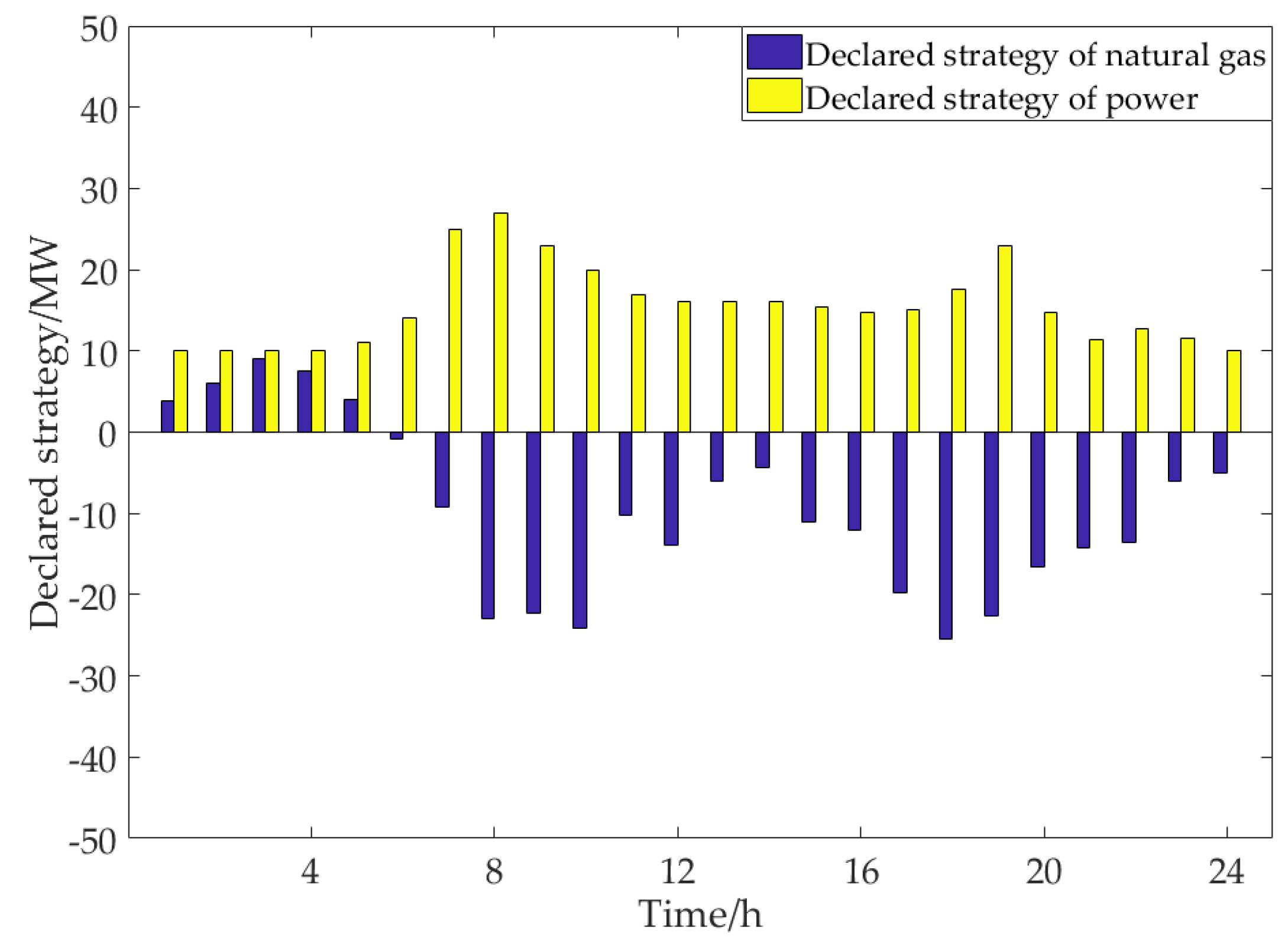
4.2. Analysis of Optimized Operation Results

In order to verify the feasibility of the model and algorithm, this paper uses Matlab R2017a to compile the model mentioned above, and carries out trial calculation, the specific MATLAB code can be seen in Supplementary Materials When $\Gamma$ = 6, the declared strategy and the optimal output power of each unit of the electric–gas interconnection system in the natural gas market and the power market in each period can be obtained, as shown in Figure 6, Figure 7 and Figure 8.

Figure 6 shows the declared strategy of the electric–gas interconnection system in each period of the natural gas market and the power market, the specific decision result data can be found in Supplementary Materials, with positive value representing sale and negative value representing purchase. As can be seen from the figure, the electric–gas interconnection system sells natural gas in the natural gas market in the periods 1–5, purchases natural gas from the natural gas market in the periods 6–24, and sells power in all the periods. In general, due to the relatively low price of natural gas, the system decision-makers in this case tend to participate in the multi energy market transaction by purchasing natural gas and selling surplus electric energy, that is, internal demand is mostly transformed into supply through purchased natural gas.

The uncontrollable component is the RE system, and the output power of electric energy in the system comes from the renewable energy units. After the output power of some renewable energy units is converted into other energy forms or supplies power to the coupling units, the remaining part is the declared value of the output power of electric energy in the system for bidding. Therefore, the optimal output power of the renewable energy units is actually the output power of the renewable energy unit ensuring the optimal purchase and sale strategy of the system, and it is not the actual output of the next day. If the decision-makers declare according to the declared strategy of energy purchase and sale corresponding to the optimal output power of the renewable energy units, the deviation of system output power will be minimized and the income will be maximized. In Figure 7, the upper and lower curves respectively correspond to the upper and lower limits of the RES output power in the system, and this value can be predicted according to the historical actual data. The shaded part is the predicted confidence interval of the RES output power within 24 h. The red curve in the middle represents the optimized RES output power strategy. It can be seen that the output power decision of RES at all times is within the confidence interval of the RES output power within 24 h, and the optimal value of the RES output power in the periods 8–9 is the upper limit value of allowable output power. According to Figure 4, Figure 5 and Figure 6, there are two factors that influence the optimal output to reach the upper limit: one is that the system power load is at the peak in the periods 8–9; the other is that the power price is at the peak in the periods 8–9. On the basis of meeting the internal energy demand, the system decision-makers sell power to the power market with the maximum capacity due to the profit seeking mentality.

In the above scenario, the output power of energy coupling unit and energy storage unit in each period of the electric–gas interconnection system is as shown in Figure 8. It can be seen from the figure that P2G equipment is in full load state all day, HP and RM are in full load state except for some periods, CHP and AR fail to reach 50% of the rated power rate in most of the periods and stay in auxiliary state, and ES is charged in the periods 3–5 and discharged in the periods 9–10 and 20.

4.3. Sensitivity Analysis

RES is the internal energy supply unit of the electric–gas interconnection system. This section discusses the influence that the change of RES output power restriction has caused on the declared strategy of the energy purchase and sale and the output power of the internal coupling unit. Under each scenario, let the upper limit of RES output power change by 20%, 10%, −10% and −20% in each period, and compare the original optimization results with the four scenarios set in this section. The expected profits of the electric–gas interconnection system participating in the market bidding under the four scenarios are shown in

Table 2. Changes in profit under four scenarios.

	Scenario 1	Scenario 2	Scenario 3	Scenario 4
Profit (EUR)	12398	12382	12150	11973
Profit change (%)	0.92	0.79	−1.1	−2.5

. The expected profit is the expected value of the profit under the probability distribution of each price sample, while the actual profit is the average value of the obtained profit assuming that a certain sample in the price sample set will actually occur.

It can be seen from the table that the expected profit generated by the system participating in the market bidding is positively related to the change of the upper limit of RES output power, and when the upper limit of RES output power changes in a negative direction, the change range of the expected profit is larger. When the upper limit of RES output power changes positively, only the optimal output power of RES in periods 8 and 9 changes (as shown in Figure 9), and when the upper limit of RES output power changes negatively, the optimal output power of RES in the periods 7–9, 11 and 19 changes simultaneously (as shown in Figure 9). Compared with the positive change, the negative change of the upper limit of RES output power is more significant, which is one of the reasons why the expected profit is more sensitive to the negative change of RES output power.

Figure 10, Figure 11, Figure 12 and Figure 13 show the bidding strategy of the electric–gas interconnection system in four scenarios and the variance ratio of the declared strategy in each period compared with the control scenario. It can be seen from the figure that under the parameter setting in this paper, when the upper limit of the internal power supply unit output changes, the internal power supply unit output changes correspondingly, but the power declared strategy does not change. Considering that the power transaction price is more advantageous than the natural gas transaction price, the system decision-makers are more inclined to reduce the natural gas declaration volume in periods 8–9 on the premise of meeting the internal load demand, so as to ensure the optimal declared strategy of energy purchase and sale. In scenario 1 and scenario 2, the power consumption of internal energy supply units is promoted by reducing the purchase of natural gas in general, and the power generation consumption of the internal energy supply unit is reduced more in the 8th period when the natural gas purchase amount is relatively large, which directly leads to the increase of expected profits. In scenario 3 and scenario 4, the power generation reduction of the internal energy supply unit is generally compensated by increasing the purchase of natural gas, and the purchase of natural gas increases substantially in the periods 7–9 and 19, which also directly leads to the reduction of expected profits.

Figure 14, Figure 15, Figure 16 and Figure 17 show the output variation ratio of the internal coupling unit in each period of the electric–gas interconnection system compared with the control scenario. It can be seen from the figure that under the parameter settings in this paper, when the upper limit of the output of the internal power supply unit in the electric–gas interconnection system changes, the output of the internal power supply unit changes correspondingly, the output of AR, P2G, RM does not change, and the output of HP and CHP changes correspondingly. In scenario 1 and scenario 2, the output of HP increases in periods 8 and 9, and the change proportion is positively related to the upper limit change of power supply unit’s output. The reason for the change is that the RES output increases in periods 8 and 9, the power declared strategy remains unchanged, and the natural gas purchase volume is reduced. When the natural gas flow and electric energy flow change, HP and CHP will change their output correspondingly to maintain the stability of heat energy flow. In scenario 3 and scenario 4, due to the increase of gas purchase volume in some time periods, CHP and HP increase or decrease their output respectively in corresponding time periods to maintain the supply-demand balance of the system. In particular, the P2G output decreases in the eighth period, and the reason is that in the controlled situation CHP output has been close to the upper limit of output in the eighth period and the increased amplitude is compressed, so P2G needs to be called to maintain the balance of supply and demand in the system.

4.4. Robustness Test

In order to verify the robustness of the declared strategy calculated by the robust optimization model constructed in this paper, this section compares the expected profit of the system with the profit conducted by determining the actual output of the next day of the system, and analyzes the economic risks of the electric–gas interconnection system under different scenarios. Without considering the output uncertainty of the electric–gas interconnection system, the predicted value of the actual system output is simply set as the average value of the historical data. When $\Gamma$ = 0, $\widetilde{P_{\mathrm{E},t,k}^{\mathrm{real}}}$, the predicted value of the actual output of the electric–gas interconnection system is equal to $\stackrel{\wedge }{P_{\mathrm{E},t}^{\mathrm{real}}}$, the midpoint of the confidence interval, and $\widetilde{P_{\mathrm{E},t,k}^{\mathrm{real}}}$ is the deterministic parameter. When considering the uncertainty of the system output, the robustness factor $\Gamma$> 0, $\Gamma$ is set to 0, 6, 12 respectively, and the actual output of the next day is assumed to be $P_{\mathrm{E}}^{\mathrm{real}}=\widetilde{P_{\mathrm{E},t}^{\mathrm{real}}}-0.5\stackrel{\Delta }{P_{\mathrm{E},t}^{\mathrm{real}}}$, this section analyzes the impact of the robustness of the model on the profit calculation results.

As shown in

Table 3. Actual profit and profit deviation of each scenario.

	$\mathsf{\Gamma }$ = 0	$\mathsf{\Gamma }$ = 6	$\mathsf{\Gamma }$ = 12
Expected profit (EUR)	12398	12285	12168
Actual profit (EUR)	6877.2	6995.8	7109.4
Profit deviation (EUR)	−5520.80	−5289.20	−5058.6

, when $\Gamma$ increases, the expected profit decreases, the profit deviation decreases gradually and the actual profit increases. When $\Gamma$ = 0, i.e. without considering the uncertainty, if the actual output of the electric–gas interconnection system deviates greatly from the power generation plan, the system may lose more profits in the day-ahead bidding, and the profit deviation will disturb the normal operation of the electric–gas interconnection system. When $\Gamma$ is 6 or 12, although the power deviation cannot be avoided and the profit deviation still exists, the profit deviation is obviously low and the actual profit is also significantly improved, which shows that considering the uncertainty in the optimization process can reduce the risk brought by the uncertainty factors to the profit. However, when considering the uncertainty of the system output, with the increase of the robustness factor $\Gamma$, the expected profit obtained by robust optimization will be reduced, so the decision-maker needs to make a reasonable decision according to his own risk tolerance.

5. Conclusions

Due to energy diversity and high coupling of the system, the bidding behavior of the electric–gas interconnection system in the market is more flexible. Considering the complementary coupling characteristics of the power system and the natural gas system, this paper uses the idea of robust optimization to establish a robust optimization model for the purchase and sale of energy in the electric–gas interconnection system in the environment of the multi-energy market based on the energy hub model. In dealing with the uncertain parameters, the cardinal uncertainty set method is used to control the deviation between the actual output and the predicted output, so as to make the overall robustness of the model controllable. The results show that:

(1)

Under the condition that the price of power is superior to that of natural gas, the system decision-makers tend to sell power and purchase natural gas to maintain the balance of supply and demand in the system and ensure the maximum bidding revenue.

(2)

The optimal bidding strategy for purchasing and selling energy, the output of the coupling unit and the expected profit of the electric–gas interconnection system are more sensitive when the upper limit of output of the internal power supply unit changes in the negative direction than when it changes in the positive direction, so the corresponding margin should be kept in the system planning.

(3)

When the robust parameter $\Gamma$ increases, the expected profit decreases and the profit deviation decreases accordingly. The decision-maker should make a reasonable decision by adjusting the robust parameter according to his own risk tolerance.

This paper focuses on the bidding strategy of the external energy purchase and sale and internal energy management of the electric–gas interconnection system, as well as the changing relationship between them, without considering the economic scheduling of the internal coupling unit. Therefore, in the next study, a refined bidding model of energy purchase and sale based on the economic scheduling of the coupling unit can be established accordingly.

References

1. Chaudry, M.; Wu, J.; Jenkins, N. A sequential Monte Carlo model of the combined GB gas and electricity network. Energy Policy 2013, 62, 473–483. [Google Scholar] [CrossRef]
2. Chen, S.; Wei, Z.; Sun, G.; Cheung, K.W.; Sun, Y. Multi-linear probabilistic energy flow analysis of integrated electrical and natural-gas systems. IEEE Trans. Power Syst. 2017, 32, 1970–1979. [Google Scholar] [CrossRef]
3. Chen, S.; Wei, Z.N.; Sun, G.Q.; Wang, D.; Sun, Y.S.; Zang, H.Y.; Zhu, Y. Probabilistic energy flow analysis in integrated electricity and natural-gas energy systems. Proc. CSEE 2015, 35, 6331–6340. [Google Scholar]
4. Cheng, L.; Liu, C.; Zhu, S.Z.; Tian, H.; Shen, X.W. Study of micro energy internet based on multi-energy interconnected strategy. Power Syst. Technol. 2016, 40, 132–138. [Google Scholar]
5. Wang, W.L.; Wang, D.; Jia, H.J.; Chenz, Y.; Guo, B.Q.; Zhou, H.M.; Fan, M.H. Steady state analysis of electricity-gas regional integrated energy system with consideration of NGS network status. Proc. CSEE 2017, 37, 1293–1305. [Google Scholar]
6. Yu, S.; Wei, Z.N.; Sun, G.Q.; Sun, Y.H.; Wang, D. A bidding model for a virtual power plant considering uncertainties. Autom. Electr. Power Syst. 2014, 38, 43–49. [Google Scholar]
7. Aghamohamadi, M.; Mahmoudi, A. From bidding strategy in smart grid toward integrated bidding strategy in smart multi-energy systems, an adaptive robust solution approach. Energy 2019, 183, 75–91. [Google Scholar] [CrossRef]
8. Zhang, Z.; Chen, Z. Optimal wind energy bidding strategies in real-time electricity market with multi-energy sources. IET Renew. Power Gener. 2019, 13, 2383–2390. [Google Scholar] [CrossRef]
9. Nojavan, S.; Zare, K.; Ashpazi, M.A. A hybrid approach based on IGDT-MPSO method for optimal bidding strategy of price-taker generation station in day-ahead electricity market. Int. J. Electr. Power Energy Syst. 2015, 69, 335–343. [Google Scholar] [CrossRef]
10. Wu, Z.Q.; Wang, T. Deviation management of wind power prediction and decision-making of wind power bidding. Power Syst. Technol. 2011, 35, 160–164. [Google Scholar]
11. Adamek, F.; Arnold, M.; Andersson, G. On decisive storage parameters for minimizing energy supply costs in multicarrier energy systems. IEEE Trans. Sustain. Energy 2014, 5, 102–109. [Google Scholar] [CrossRef]
12. Neyestani, N.; Yazdani-Damavandi, M.; Shafie-Khah, M.; Chicco, G.; Catalao, J.P.S. Stochastic modeling of multienergy carriers dependencies in smart local networks with distributed energy resources. IEEE Trans. Smart Grid 2015, 6, 1748–1762. [Google Scholar] [CrossRef]
13. Wang, Y.; Zhang, N.; Kang, C.; Kirschen, D.S.; Yang, J.; Xia, Q. Standardized matrix modeling of multiple energy systems. IEEE Trans. Smart Grid 2019, 10, 257–270. [Google Scholar] [CrossRef]
14. Ma, T.F.; Wu, J.Y.; Hao, L.L.; Li, Y.J.; Yan, G.H.; Li, D.Z.; Chen, S.S. Energy flow modeling and optimal operation analysis of the micro energy grid based on energy hub. Power Syst. Technol. 2018, 42, 179–186. [Google Scholar] [CrossRef]
15. Jia, H.J.; Wang, D.; Xu, X.D.; Yu, X.D. Research on some key problems related to integrated energy systems. Autom. Electr. Power Syst. 2015, 39, 198–207. [Google Scholar]
16. Pu, F.P.; Tian, S.M.; Fang, F.; Ying, K.; Du, W.Q. Optimal day-ahead scheduling method for hybrid energy park based on energy hub model. Proc. CSU EPSA 2017, 29, 123–129. [Google Scholar]
17. Bertsimas, D.; Litvinov, E.; Sun, X.A.; Zhao, J.; Zheng, T. Adaptive robust optimization for the security constrained unit commitment problem. IEEE Trans. Power Syst. 2013, 28, 52–63. [Google Scholar] [CrossRef]
18. Zhao, L.; Zeng, B. Robust unit commitment problem with demand response and wind energy. In Proceedings of the 2012 IEEE Power And Energy Society General Meeting, San Diego, CA, USA, 22–26 July 2012. [Google Scholar]
19. Wei, W.; Liu, F.; Mei, S.W. Robust and economical scheduling methodology for power systems: Part two application examples. Autom. Electr. Power Syst. 2013, 37, 60–67. [Google Scholar]
20. Wei, W.; Liu, F.; Mei, S.W. Robust and economical scheduling methodology for power systems: Part one theoretical foundations. Autom. Electr. Power Syst. 2013, 37, 37–43. [Google Scholar]
21. Yu, D.W.; Yang, M.; Zhai, H.F.; Han, X.S. An overview of robust optimization used for power system dispatch and decision-making. Autom. Electr. Power Syst. 2016, 40, 134–143. [Google Scholar]
22. Pu, L.; Wang, X.; Tan, Z.; Wu, J.; Long, C.; Kong, W. Feasible electricity price calculation and environmental benefits analysis of the regional nighttime wind power utilization in electric heating in Beijing. J. Clean. Prod. 2019, 212, 1434–1445. [Google Scholar] [CrossRef]
Figure 1. Typical structure of the electric–gas interconnection system.
Applsci 09 05497 g001
Figure 2. Bidding process of Nordic power market.
Applsci 09 05497 g002
Figure 3. The process of k-means algorithm clustering.
Applsci 09 05497 g003
Figure 4. Scenario data of typical daily price.
Applsci 09 05497 g004
Figure 5. Load data of the system.
Applsci 09 05497 g005
Figure 6. Optimization results of system declared strategy.
Applsci 09 05497 g006
Figure 7. Optimization results of the output power in the renewable energy system (RES) system.
Applsci 09 05497 g007
Figure 8. Optimization results of the output power in the coupling unit.
Applsci 09 05497 g008
Figure 9. Variation results of the output power in the RES system.
Applsci 09 05497 g009
Figure 10. Variation results of declared strategy in scenario 1.
Applsci 09 05497 g010
Figure 11. Variation results of declared strategy in scenario 2.
Applsci 09 05497 g011
Figure 12. Variation results of declared strategy in scenario 3.
Applsci 09 05497 g012
Figure 13. Variation results of declared strategy in scenario 4.
Applsci 09 05497 g013
Figure 14. Variation results of the coupling unit output power in scenario 1.
Applsci 09 05497 g014
Figure 15. Variation results of the coupling unit output power in scenario 2.
Applsci 09 05497 g015
Figure 16. Variation results of the coupling unit output power in scenario 3.
Applsci 09 05497 g016
Figure 17. Variation results of the coupling unit output power in scenario 4.
Applsci 09 05497 g017