Path Planning under Force Control in Robotic Polishing of the Complex Curved Surfaces

Abstract

Surface polishing is required in many manufacturing sectors. Currently, it demands a large amount of manual work, which is time-consuming, error-prone, and costly. Additionally, it creates hazards for the workers as it may result in many deadly respiratory diseases. Robotic polishing is the solution to these problems. It can improve productivity, eliminate the defects, and provides consistent product quality. In this paper, an effective approach is presented for the robotic polishing of the complex curved surfaces. The key part of the presented method is the tool path planning with controlled force and polishing parameters optimization evaluated using design of experiments (DOE). The tool path planning is aimed at improving the surface quality and the contact area per path. The constraints of joint limits and productivity are also considered. Moreover, its jerk avoidance strategy allows the robot to move swiftly while ensuring a smooth trajectory. The presented method is verified for the polishing of an eyeglass frame. A considerable improvement of 90% on the average roughness is achieved with the maximum acceptable roughness set at 0.02 µm. The polishing operation takes just 79 secs and the average glossiness of 76 G is achieved on the final product along with the successful elimination of scratches on the surface.

1. Introduction

Polishing is a tedious but important finishing process, which demands a considerable amount of manual work in many manufacturing sectors. It is equally essential in the restoration of the old or damaged parts. This time consuming, error-prone, and costly multistage process is facing a shortage of skilled workers due to the various problems, such as government regulation, deadly respiratory diseases, and increasing labor cost [1,2,3,4]. Robotic polishing is the solution to these problems, which can improve the working condition of the labor, eliminate the manufacturing defects, and ensure the product quality giving an appealing glossiness to the product.

As a serious contender for the robotic polishing, the industrial robot is an automated, programmable, and multipurpose robotic system, which can work in unhealthy and accident-prone environments with high accuracy. However, it has some mechanical constraints, which need to be addressed before using it into the surface polishing of the complex parts. For instance, even for the simplest movement of the end effector between two points within the working envelope requires proper consideration of collision avoidance, work proficiency, best obtainable trajectory path, and other kinematic constraints such as singularity and joints limits. Therefore, path planning and trajectory planning are very significant for robot movement.

Moreover, cumulative demand for high speed and less production time from the industrial robots challenge high precision and repeatability. These extreme demands place the path and trajectory planning algorithms in the limelight. Path planning utilizing various scanning patterns and space-filling curves have been discussed under automated polishing in several research studies [5,6,7,8,9]. H. Y. Tam et al. presented an investigation for surface roughness reduction by using a scanning path, which focuses the path evenness through pitch adaptation with surface slope changes and line spacing [5]. Fractal path generation was used in the robotic polishing of the metal molds [6]. It used a planer Peano curve with end effector orientation normal to the freeform surface. Contact mechanics was also used for contact area modeling and analysis to automate the polishing process in coverage based tool-path planning [7].

Similarly, the different force control methods and process control techniques have been used for better-controlled interaction during the polishing [10,11,12]. A fuzzy vector method was suggested for the grinding and polishing, which enables the controller to deal with force sensor signals caused by the working tool, to search the direction of the constraint surface of an unknown object [10]. Another study concentrated on the control issues that arise during the automation of die and mold surface polishing using an arm robot, particularly on the force controllers to maintain the required tool and workpiece interaction [12]. The major focus of this paper was on the active end effector force control because there are performance limitations in the force control loop of the arm robot.

The third most adopted technique for the improvement of automated polishing is the implementation of specially designed polishing tools [13,14,15]. Chunjin Wang et al. presented an improved semirigid bonnet tool for the high-quality polishing on aspheric optics [13]. Based on the finite element analysis method, the tool influence function is modeled for the structural optimization to eliminate previous present defects. In paper [15], a collaborative tool for robotic polishing was presented to allow the simultaneous operation of the robot and human cooperation for polishing. The polishing tool was developed by using the minimum viable product approach.

However, tool path planning plays a significant role in achieving the good surface quality during the polishing process in the complex structures and requires high reachability, but it offers some relaxation in terms of accuracy [11]. Due to the flexibility and dexterity of the articulated robot, it is a better preference for polishing the non-plainer surfaces as compared to other types of industrial robots. It can be programmed for surface polishing by specifically repeated action with acceptable accuracy.

This paper presents a tool path planning approach to polish the complex curved surfaces utilizing a six-axis industrial robot under controlled and optimized force. The key contribution of the paper is to combine the path planning, the force control, and the optimization of the polishing parameters for polishing complex surfaces, such as an eyeglass frame, to achieve the desired surface quality efficiently. The optimization of the polishing parameters is obtained using the full factorial design of experiments (DOE). Common path planning issues like joint limits and the singularity of the robots are also addressed since these are part of path planning. Surface quality judgment parameters like glossiness, surface roughness, and scratch eradication on the surface area under the proposed method are tested for polishing an eyeglass frame to verify the anticipated methodology. The proposed method gives complete insight into the automated polishing and can improve the complex curved surfaces quality effectively.

The rest of the paper is organized as follows: Section 2 presents the proposed method with focuses on force controlling strategy, tool path planning, and method to evaluate the optimized polishing parameters. Section 3 gives the experiment setup, the testing results, and discussions. Finally, Section 4 contains conclusions.

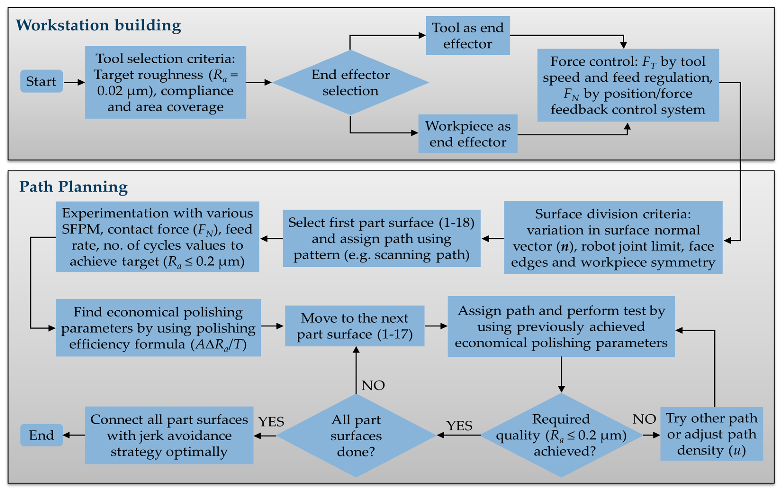
2. The Proposed Method

The key to robotic polishing is the tool path. Ideally, it shall have the minimum path length, the best coverage of the polishing surface and the uniform surface quality. A top-down approach is developed for tool path planning. Figure 1 shows the setup for the robotic polishing of the eyeglass frames, which includes an articulated robot with a supporting fixture to hold the workpiece and a force feedback system to control the polishing force of the tool through a variable speed motor.

The flow chart of the proposed robotic polishing method for the complex curve surfaces is presented in Figure 2. It consists of two major stages (workstation building and path planning). In the workstation building stage, polishing tool selection, decision for using a tool or workpiece as the end effector, and force controlling strategy are determined because these decisions affect the tool path planning. Path planning can be further divided into three stages. First is surface division, in which the surface to be polished is divided into several regions. For each region, the limits of the robot joints and surface normal vector are considered to ensure continued orientation. Second is tool path generation, in which each surface region is assigned a tool path with specific pattern and polishing parameters. The quality of the polishing surface and productivity are the major considerations here. Finally, the tool path stitching, in which the tool paths in different regions are stitched together. The major considerations include the shortest connecting routes and jerk avoidance. These parts are detailed below.

2.1. Workstation Building and Force Control

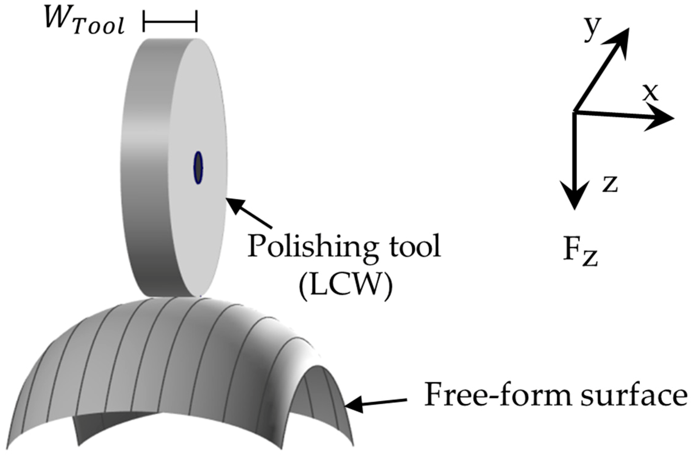
2.1.1. Polishing Tool and End Effector Selection

There are large amounts of polishing tools available in the market. To select an appropriate tool would need to consider various factors such as tool cost, required roughness, polishing time, tool changing time, tool compliance, material removal rate, etc. [16]. For polishing plain and/or simple curved surfaces, it is relatively easy to find a suitable tool that can reach every point of the workpiece. However, for complex surfaces, it is sometimes difficult to find a perfect tool. A sensible solution is to test several polishing tools manually on the workpiece. In our application (polishing eyeglass frame), based on the know-how of experienced workers, we choose the 150 mm × 15 mm loose cotton wheel (LCW) for polishing (Manufacturer: Bolpol, Model: HL150/1) with dry polishing wax. It is a flexible polishing tool that can reach the difficult corners of the eyeglass frame. The target is to achieve the arithmetic average roughness ($R_a$) of 0.02 µm.

For robot polishing, the end effector of the robot can be either the polishing tool or the workpiece. The decision depends on the application [17,18,19,20]. Figure 3a shows the polishing tool used as the end effector. It is effective when the workpiece is large and/or heavy. Additionally, when multiple polishing tools are needed, it is convenient to use an automatic tool changer (ATC) for tool change. In other configurations, workpiece is used as an end effector by attaching to the robot through a specifically designed fixture as shown in Figure 3b. The advantage of this setup is that the orientation of the end effector can be easily controlled to retain a constant orientation between the tool and the workpiece. Additionally, the polishing force control unit can be separated from the robot and there is no delay in polishing for the various tools change. Thus, in this study, the workpiece is used as an end effector.

Note that when using a workpiece as the end effector, both the payload and the gripping force of the robot must be considered. The payload is the maximum mass that can be attached as the end effector of the robot. It is a key parameter when selecting the robot, whereas, the gripping force is the maximum force of the gripper to hold the workpiece as

$$F_g=\frac{m_g(g+a)}{\mu }$$

(1)

where $F_g$ is the minimal gripping force to hold the workpiece, µ is the friction coefficient, g is the gravitational constant, m_g is the mass of the gripped body and a is the acceleration. In the polishing operation, the tool exerts force on the workpiece to smoothen the surface. This additional polishing force $\left(F_p\right)$ must be added in the gripping force to firmly hold the workpiece during the polishing process. Hence, the total gripping force (F_t) can be represented as

$$F_t=F_g+F_p=\frac{m_g(g+a)}{\mu }+F_p$$

(2)

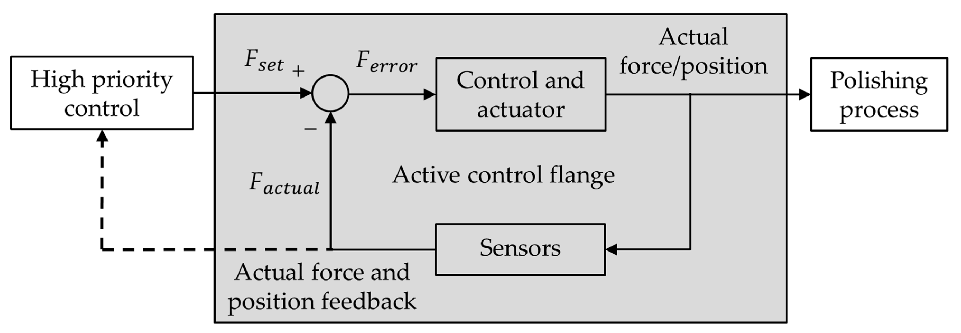
2.1.2. Force Control in Surface Polishing

During the grinding and polishing process, the interacting force between the tool and surface plays a key role in achieving the surface finish. Generally, this force can be divided into two components, which are tangential force component ($F_T$) and normal force component ($F_N$) [21,22,23] as shown in Figure 4a. The direction of the $F_T$ is parallel to the direction of the feed and affects the power consumption and tool life, whereas the direction of $F_N$ is perpendicular to the surface plane and it has more influence on surface roughness and deformation of the workpiece [21]. A threefold strategy is presented in Figure 4b, which controls all three factors (wheel rotation speed, workpiece speed and direction, and normal contact force), which affect $F_T$ and $F_N$.

Tangential Force Component Control

Specific grinding energy (u) is an important process parameter, which can be defined as the energy consumed per unit volume of material removed [21,22], it can relate $F_T$ and other parameters as

$$u=\frac{F_T{v}_s}{v_w{a}_{p}b}$$

(3)

where b is the width of the wheel and $a_p$ is the depth of the cutting (for polishing less material removal is always desired so it will be very shallow). The other two parameters are wheel speed ($v_s$) and workpiece speed ($v_w$), which are used to control the $F_T$ in this work.

Wheel speed or surface feed per minute: the polishing wheel speed against the normal polishing force (pressure applied on the workpiece) is very important for effective polishing. It is measured by surface feet per minute (SFPM), which dependents on the wheel diameter and the wheel rotation speed:

$$SFPM=\mathsf{\pi }\left(\frac{1\left(ft\right)}{12\left(in\right)}D\right)\mathrm{rpm},$$

(4)

where D is the diameter of the wheel in inches (in) and rpm is the speed of the wheel (revolutions per minute). From the SFPM formula, it can be seen that the required SFPM can be achieved with the various combination of the wheel diameter and the wheel rotation speed. Depending on the SFPM, the wheel creates a frictional force for the polishing process that can be further tuned by the applied pressure from the normal contact force.

Workpiece speed and direction: the workpiece speed and direction against wheel rotation are other factors that contribute to polishing force. The direction of workpiece motion plays a significant role in handling the applied pressure. There are two motions for the polishing as shown in Figure 5. The first one is moving the workpiece against the wheel rotation with high pressure. It is usually used for smoothening and can generate the semi-brightness surface. The second motion is moving the workpiece in the direction of the wheel with comparatively medium or low pressure. It produces brightness and a shiny surface.

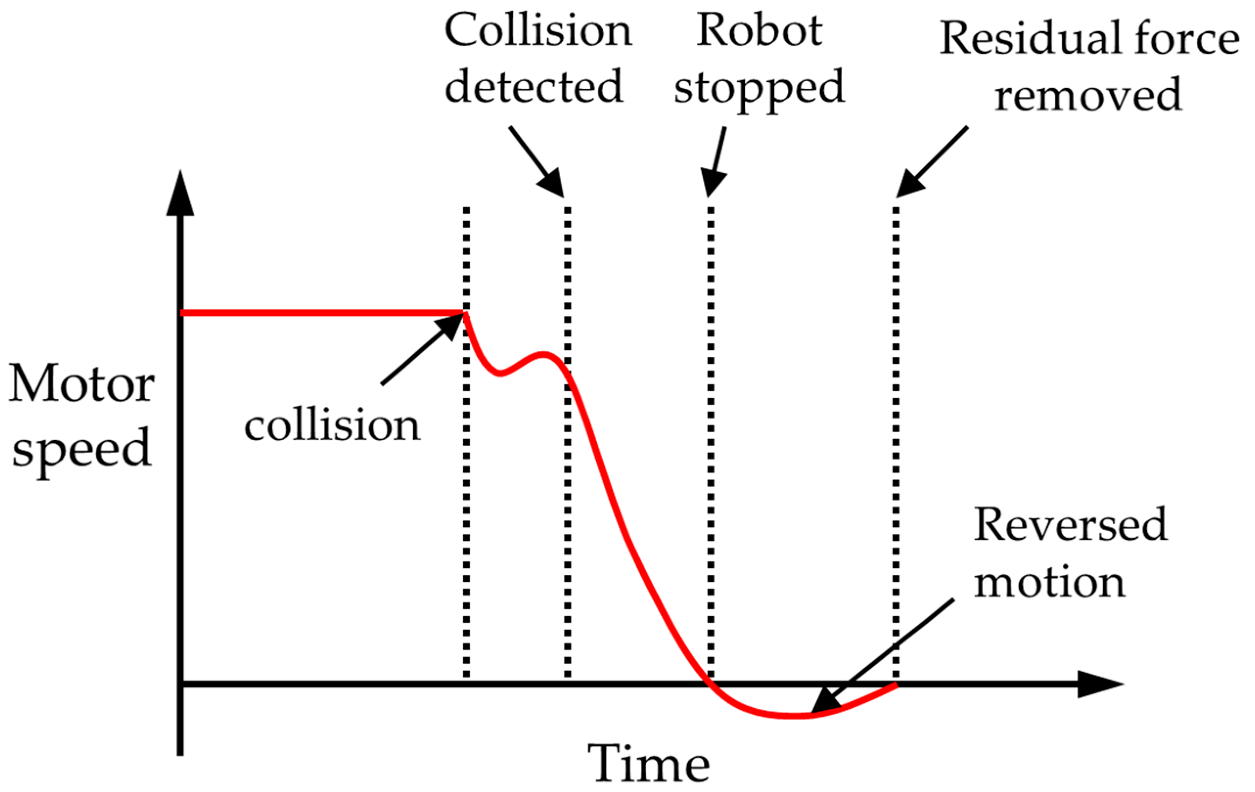
Normal Force Component Control

In order to achieve the full control of the polishing force, merely aligning up the workpiece and the speed regulation of the tool and workpiece is not enough, particularly when the workpiece has a freeform surface. Therefore, a force feedback control system active contact flange (ACF) manufactured by Ferrobotics under model ACF110-01 is used to keep the contact force constant. It shall be mentioned that many force feedback systems in robot applications use only one extensive setup to control the force and position because robot movement is associated with it [24,25,26]. It may cause a delay in the response of the force regulation. Conversely, ACF uses a separate setup independent of the robot movement, which provides quick response time. Therefore, the presented system has two different setups for robot force and motion control.

The first setup has a robot and its controller for the robot movement and collision control. It uses motion supervision, which is a highly sensitive feature in robot for the supervision of load, jam, and collision. If it is kept very sensitive, the movement may trip for a large force acts on the robot. Depending on the polishing process force, the sensitivity level should be raised until no trigger occurs. If any collision detected under the sensitivity level, the robot will quickly stop and move back a short distance to remove residual forces as shown in Figure 6.

Another separate setup is for ACF, which controls the normal contact force. The block diagram of the ACF setup is shown in Figure 7. It is a hybrid position/force control system. It consists of a high priority control and a core force feedback regulation unit. Its Ethernet-based interface allows the user to set the desired force and constantly provides the status of the actual force and position displacement.

ACF does not interfere in the predefined robot movement and uses the sensor-based feedback to measure output force and position. Any error (F_error) between set force (F_set) and actual force (F_actual) can be found by comparing these forces as in Equation (5). The corrected force and its corresponding position are asserted by an autonomous pneumatic actuator, which quickly compensates any abrupt change in the force and provides dexterity and sensitivity for high-speed precision surface treatment. Additionally, it offers gravitation compensation and provides constant force even with changing orientations if it is used at the robot end effector.

$$F_{error}=F_{set}-F_{actual}.$$

(5)

It is important to note that ACF is a one-dimensional system. When polishing a freeform surface as illustrated in Figure 8, the workpiece surface must be constantly moved by the robot against the polishing tool so that the polishing force remains normal to the tool. The width of the polishing wheel (W_Tool) covers the workpiece surface strip by strip. This proposed setup separates the control of the workpiece position (through the robot) and the control of the polishing force (through the polishing wheel). It has two advantages: first, the passive nature of the end effector avoids mechanical vibrations generated due to the motor rotation. Second, the force control does not affect the payload of the robot and hence, it is easy to implement.

2.2. Tool Path Planning

The presented path planning for a multifaceted eyeglass frame consists of three major parts: surface division, path planning for each part surface, and stitching of all part surfaces in one trajectory.

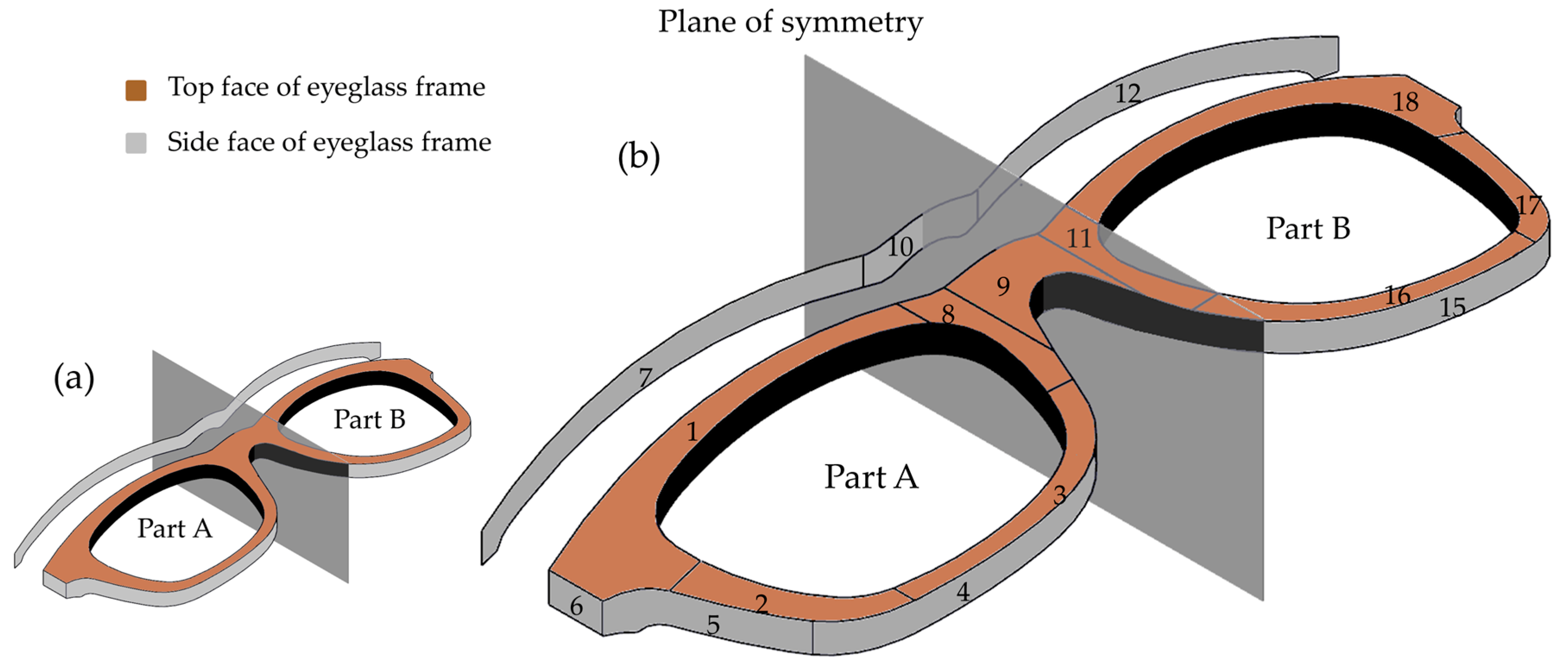
2.2.1. Surface Division

It is known that the robot reachability at a point with a particular orientation of the end effector or tool frame {T} depends on its joint configuration q = {q_j, j ∈ [1 … N]} ∈ ϐ, where q_j the joint configuration, N is the number of joints, and ϐ is configuration space. In three-dimensional space, minimum six joints are needed to position the {T} because the object in space requires six parameters, three from ${\mathrm{ℝ}}^3$ (coordinates of the origin of the attached frame), and three from SO(3) (rotation matrices for frame orientation) such robots are said to have six degrees of freedom [27]. The articulated robot with end effector poses ξ_E~(x, y, z, θ_r, θ_p, θ_y) fulfills this demand.

However, maintaining the required position and orientation continuously normal to the surface may not be feasible due to the joints limit. To achieve the non-stop smooth trajectory for the entire polishing surface, it is often necessary to divide the polishing surface into several regions. It converts a complex surface into several simple curved surfaces, which is comparatively easier to polish. It also helps to provide better tool contact with the workpiece surface, which improves the polishing quality. Moreover, it offers a quick change in the tool path of the particular area when needed without disturbing the other part surfaces.

In this study, the symmetrical eyeglass frame is first divided virtually into two symmetrical parts A and B by the plane of symmetry as shown in Figure 9a. The surface division in one part shall be followed in the other part by mirroring. Secondly, the surface is further divided into the top and side face by following the edges of the faces. Additionally, other multiple factors are considered including the variation in the orientation of surface normal vector (n), the robot joints limit, the curvature of the part surface, the size, and complexity of the face. By taking these factors into account, the eyeglass frame is divided into 18 plain and simple curve part surfaces as in Figure 9b. Most of the parts are simple in shape with less n variation. Part surface 1–8 and 11–18 are symmetrical, therefore, the polishing tool will follow a similar tool path.

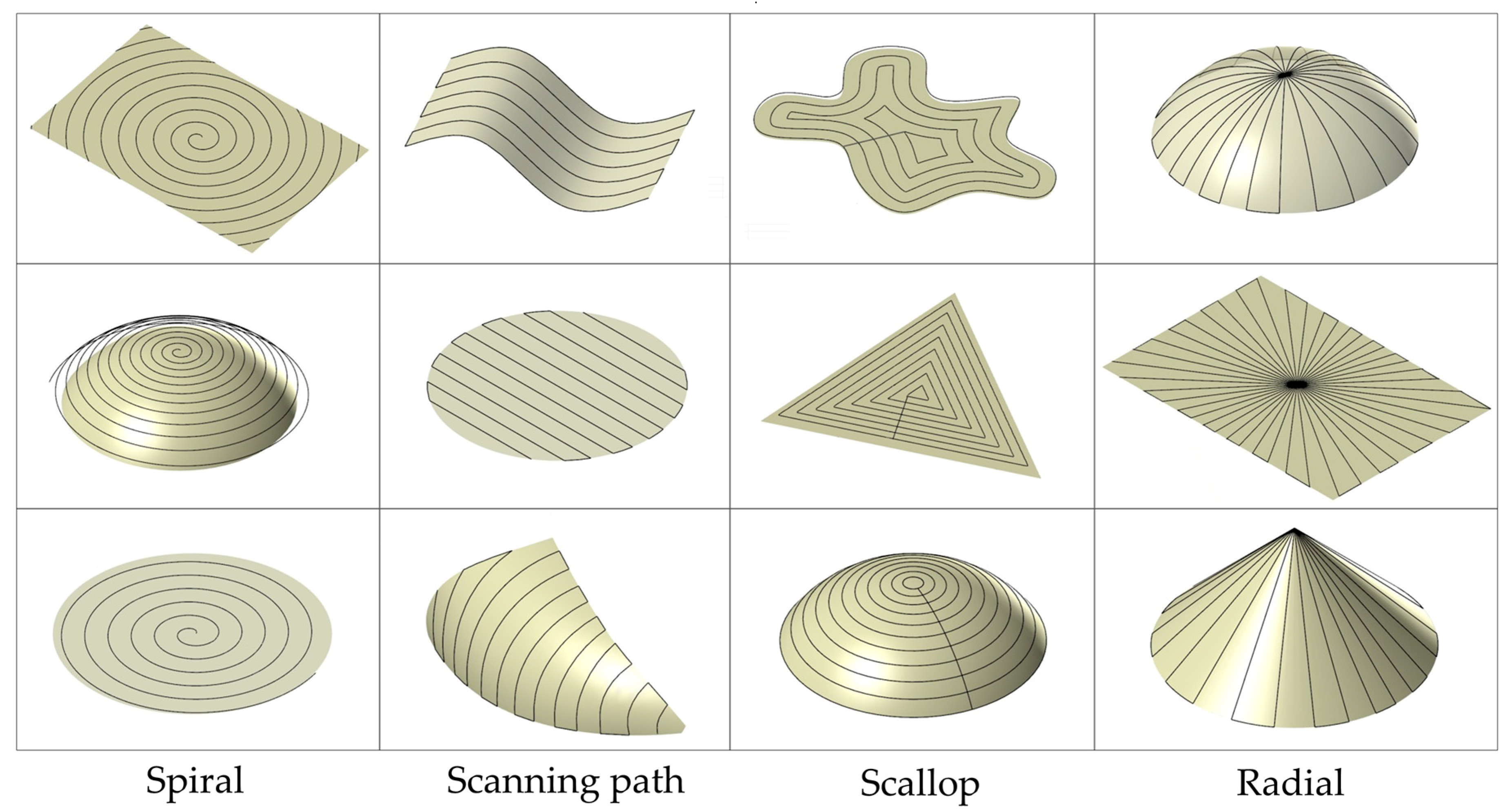
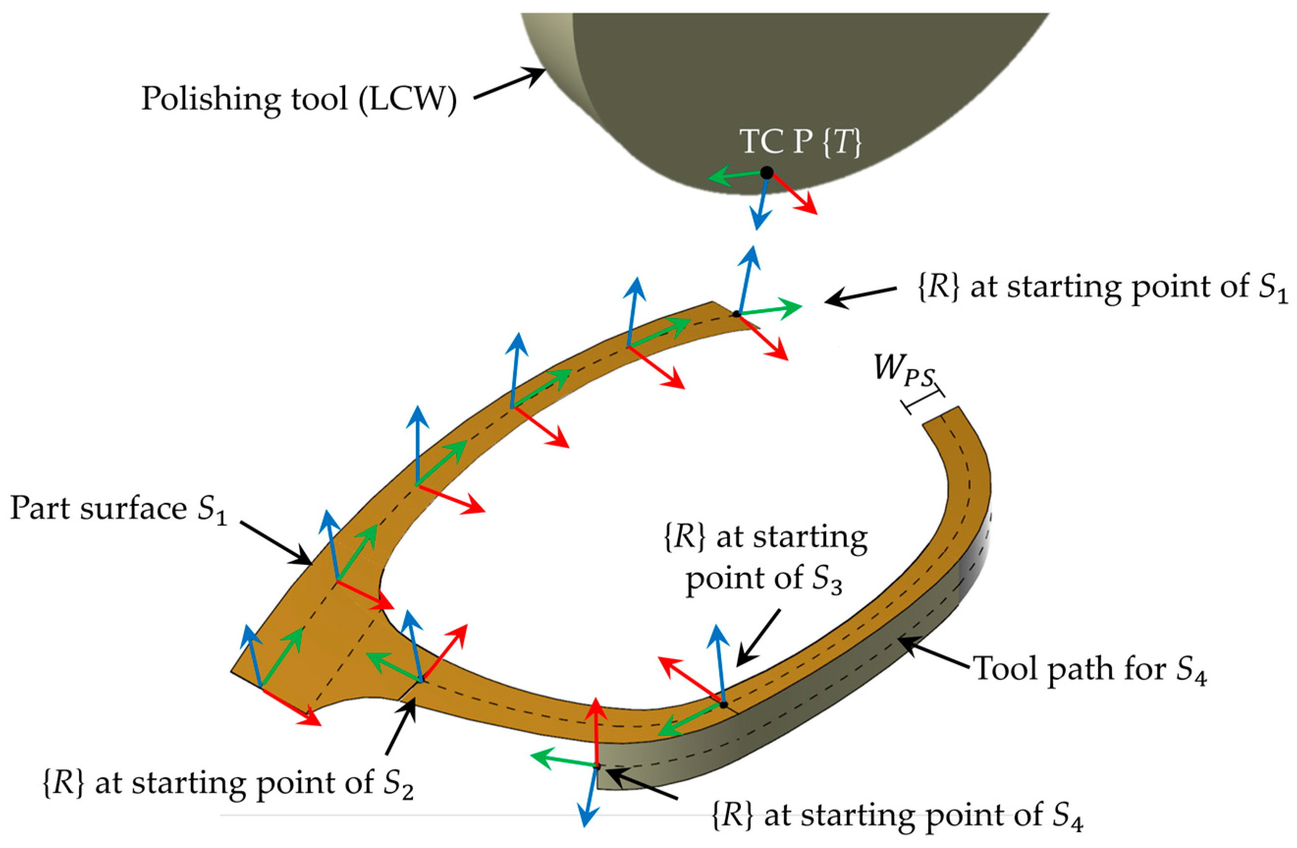
2.2.2. Tool Path Generation for Individual Part Surfaces

Tool path pattern: the prime objective of path planning is the achievement of the required level of the surface finish on the entire area of the workpiece in the shortest time. Several scanning patterns and area filling curves have been implemented on the different shapes of the workpieces for the better path consistency, stock removal, surface texture, and quality [5,6,28,29]. Figure 10 presents some commonly used tool path patterns to cover the plain or simple curved surfaces. Each pattern has its advantages, disadvantages, and parameters that control its performances.

According to the literature, the scanning path is one of the most adopted tool path patterns in polishing [5,8,9,30,31]. In this study, the scanning path pattern was selected for the eyeglass frame because mostly part surfaces were long stripes. Scanning path consists of a starting point, ending point, and the middle body. It can be classified into two categories, “S” pattern and “Z” pattern. Path density of the middle body is responsible for the quality and the productivity of the polishing process that can be controlled by the distance between two consecutive lines. In S scan, tool moves in an alternative direction, however, Z scan moves in the same direction all over the scans. In tangential polishing, tool feed direction had a significant impact on the resultant surface as discussed in Section 2.1.2. The implementation of the scanning path patterns for the polishing curve surface utilizing adopted LCW can be seen in Figure 8. High curvature surfaces demand high path densities because these provide less surface contact. Depending on the tool effective width ($w_e$), line spacing can vary from 0 to W_Tool.

Tool compliance: the flexibility of the polishing tool is another important factor that offers smooth interaction, additional tool contact, and help to reach the difficult places of the workpiece. Examples of flexible tools include polishing belts, wool pad, and cloth wheels. Figure 11 shows the impact of using different tool center point (TCP) at flexible LCW in polishing the plain and simply curved surface.

TCP defines the zero position of the tool coordinate system. All robots have predefined tool coordinates system and new tool coordinates are defined as an offset from this predefined location. TCP with R–h gives large surface contact compare to TCP at R. However, it offers different effects on plain and curved surfaces ($a_2>a_1$) as shown in Figure 11b,c. Smart surface division can convert the high curvature surfaces into nearly a plain or less curved surface that can provide approximately the same contact area as plain surface (i.e., $a_2\cong a_1$). Equation (6) affirms that $w_e$ and s controls the surface contact area ($A_C$) between the tool and plain surface. In our study, TCP is taken at R–h with a small value of s because the compliance force of the tool can easily deform the frame for a larger value.

$$A_C=2w_e(R-h)tan(\raisebox{1ex}{${\theta }_1$}\!\left/ \!\raisebox{-1ex}{$2$}\right.)\mathrm{and}{\theta }_1={cos}^{-1}\left[\raisebox{1ex}{$(R-h)$}\!\left/ \!\raisebox{-1ex}{$R$}\right.\right].$$

(6)

TCP or end effector velocity in polishing: the composite robot applications like painting, welding, and polishing require continuous path control with explicit orientation and uniform velocity. Within the working space of a robot, there are some spaces where the position and orientation of the end effector of the robot cannot be asserted. These locations are referred to as singularities in which robot displacements and velocities are volatile [32]. For the six-axis robot, singularity can be mathematically described by the relation between the vector of joint velocities ($\dot{q}$) and the Cartesian velocity vector (v) of the end-effector [27].

$$q=J^{-1}v,$$

(7)

where J is a Jacobian matrix of order 6 × 6, which is a function of the joint positions (q) and the robot geometry. This equation can calculate joint rates at every point on the path for the robot movement with some velocity vector in the Cartesian space. However, the robots have some values of q for which Jacobians becomes singular. Those places are considered as singularities.

While using the robot in Cartesian mode, trajectories that instruct the robot to move close to a singularity must be avoided. Normally, robots are programmed to stop the movement near singularity to avoid any harm to the robot. Some robots are designed to move slowly near a singularity but lose constant speed in line and force the tool to linger on at the same point, which is damaging for the polishing surface. Sometimes to avoid the most commonly occurred wrist singularity, a small angle is added to the end effector, which reduces the chance of two links alignment.

Optimization of polishing parameters: optimized control of the polishing parameters can lead to the required surface quality (surface roughness R_a) in a short time. However, it is difficult to optimize the input parameters due to the complexity of the polishing process. Additionally, the random effects of the flexible polishing tool on the polishing surface make this process difficult to represent by simple equations. Therefore, a full factorial DOE is used to investigate the effect of input factors (SFPM, feed rate, and no. of the polishing cycle) on the surface roughness of the eyeglass frame in the polishing process. It can help to find the economical polishing parameters for the required surface finish. The full factorial design consists of all possible combinations of the input factors and their levels [33,34]. The number of the experimental run for a full factorial design is the product of the levels of each factor ($F_n$):

$$No.ofexperimentalrun=Levelsin{F}_1\times Levelsin{F}_2\times \dots \times Levelsin{F}_n.$$

(8)

Using the above equation, thirty no. of experimental runs were designed with the various combinations of the process parameters. Besides the full factorial design, other methods under DOE can be used such as the fractional factorial design, Plackett–Burman design, and Taguchi method. However, depending on the required accuracy and process cost a full factorial design is used.

$$PE=\frac{{A\Delta R}_a}{T}$$

(9)

According to references [29,30], the best parameters can be selected by using the polishing efficiency (PE) formula given in Equation (9). It is defined as the amount of roughness reduction (∆$R_a$) for the specified area (A) in time (T). A plot of the PE against the $R_a$ can help to extract the best possible polishing parameters based on the highest polishing efficiency achieve.

After the surface division of the eyeglass frame, most of the part surfaces are strips. The maximum width ($W_{PS}$) of each part surface is less than the tool width ($W_{Tool}$). As a result, the polishing tool can cover the entire strip or part surface just in one pass starting from one point and ending at the opposite side. However, to achieve the required surface quality, multiple polishing passes are needed. The number of polishing passes, the starting, and ending points is dependent on the polishing parameters. Figure 12 shows the polishing trajectory of the four part surfaces with the tool and robot target frames {R}. Based on the optimized polishing parameters achieved by full factorial DOE from the part surface one ($S_1$), two polishing cycles are suggested for each part surface. In the first polishing cycle, the eyeglass frame will move against the wheel rotation and later in the direction of the wheel rotation for required gloss. {T} will remain normal to the surface during the whole polishing process.

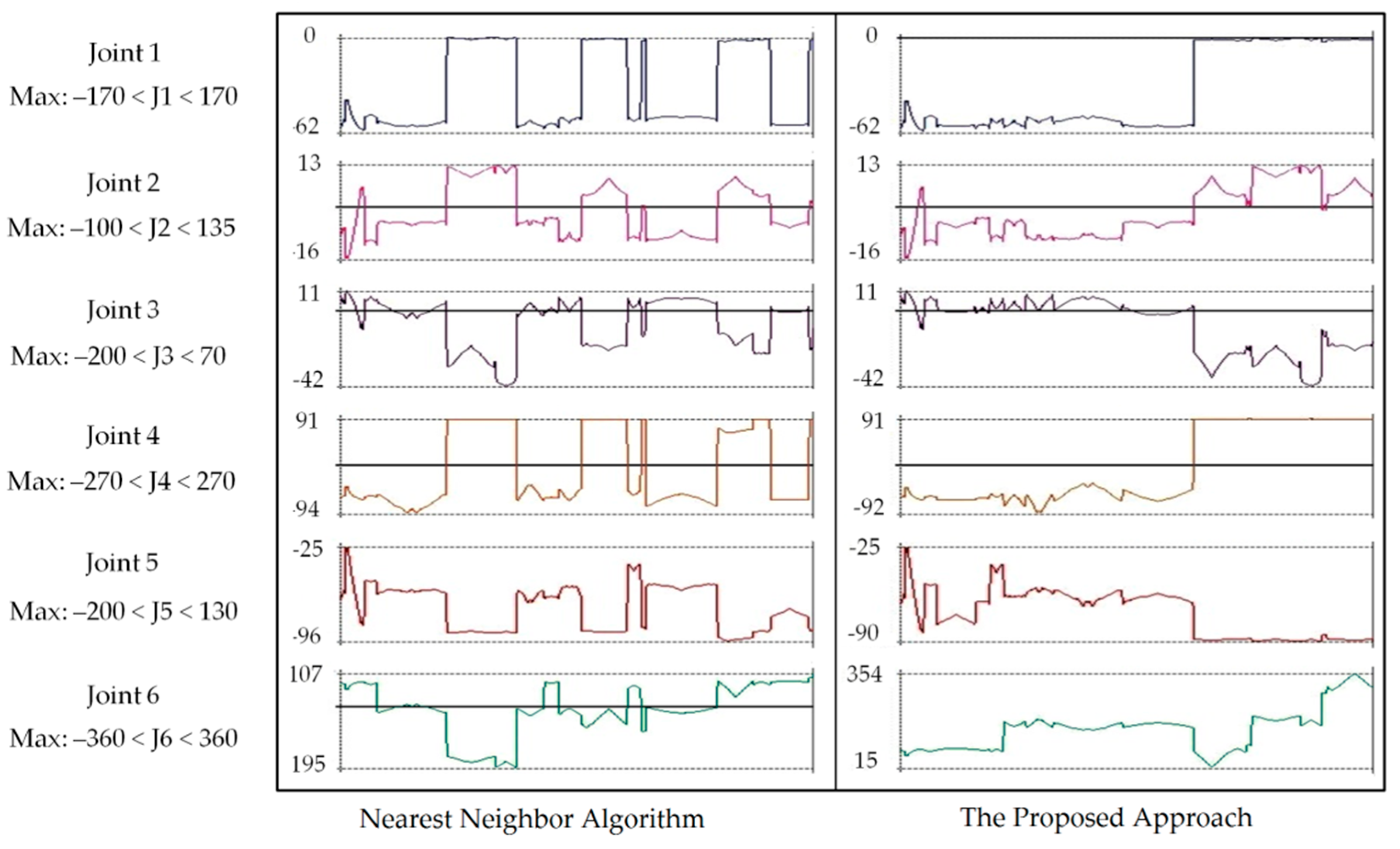
2.2.3. Tool Path Stitching

The final step is to link all the part surfaces to achieve the shortest possible route, minimum joint angles, and jerk-free movement. Previously [9], the shortest possible connecting route was achieved by using brute force search, nearest neighboring algorithm (NNA), and the greedy algorithm. These algorithms do not satisfy the target of achieving the smooth robot movement with minimum joint angles because they just focus to find the shortest connecting distance. Therefore, a new approach was used here, which satisfies all the mentioned objectives.

The proposed strategy avoids the hasty orientation shifts during the connecting path movement. It sorts part surfaces in different groups based on the orientation of the {T} at the starting point in each part surface. Following the surface division previously as in Figure 9, there are two face groups (top and side). The total 18 part surfaces of the eyeglass frame are mainly sorted into top and side face groups. Similarly, the top face group is further sorted into the X-axis and Y-axis categories. Later, the part surfaces in the X-axis group are linked based on minimum Euclidian distance d(p, q) as express in Equation (10). The same action is performed on the other two sorted groups. Finally, all these three groups are connected to create one complete path based on the short distance covered.

$$d(p,q)=min\sqrt{{(p_1-q_1)}^2+{(p_2-q_2)}^2+{(p_3-q_3)}^2}.$$

(10)

Figure 13 compares the effect of using the NNA and proposed approach to connect the part surfaces by showing the complete joints angle movement (${\theta }_n$: n = 6) of the robot during the polishing of the eyeglass frame. Both methods utilized only an average of 32% of whole angles range available for the used robot because of the smart part division approach. However, the new proposed strategy allows the robot to maintain {T} orientation normal to the surface during polishing by using very less joints movements. Additionally, it provides smooth robot movement because it avoids a jerk, which occurs due to the sudden tool orientation shift while moving from one part to another part surface and hence, allows the robot to move comparatively faster. Moreover, the Joint 4 (wrist) demonstrated a minimum and smooth angle transition that was significant in avoiding the mostly occurred wrist singularity.

3. Results and Discussions

A compact ABB IRB 1200 six-axis industrial robot controlled by IRC5 controller polishing the eyeglass frame is shown in Figure 14. It can carry 7 kg payload, which is enough to support the eyeglass frame fixture during polishing. A separate setup for force regulation (ACF110-01) was used independently for the robot movement as discussed earlier. Motor-driven polishing wheel (LCW) was attached to the force sensor, which was present in front of the robot within its working envelope. A well planned off-line tool path planning under the proposed method and its conversion into its corresponding robot joint angle values was performed using robot programming simulator Robotmaster^®. Flex pendant with the small LCD was used for different operations of the robot system such as jogging the robotic arm, running, and a quick modification in the robot program.

Figure 15 shows the different equipment used for surface evaluation of the eyeglass frame. These are a surface roughness tester (SJ-210), a special purpose (small aperture) gloss meter (NHG60M) with a 60° measuring angle, and a highly zoomed microscope. A tachometer was used for the tool speed measurement.

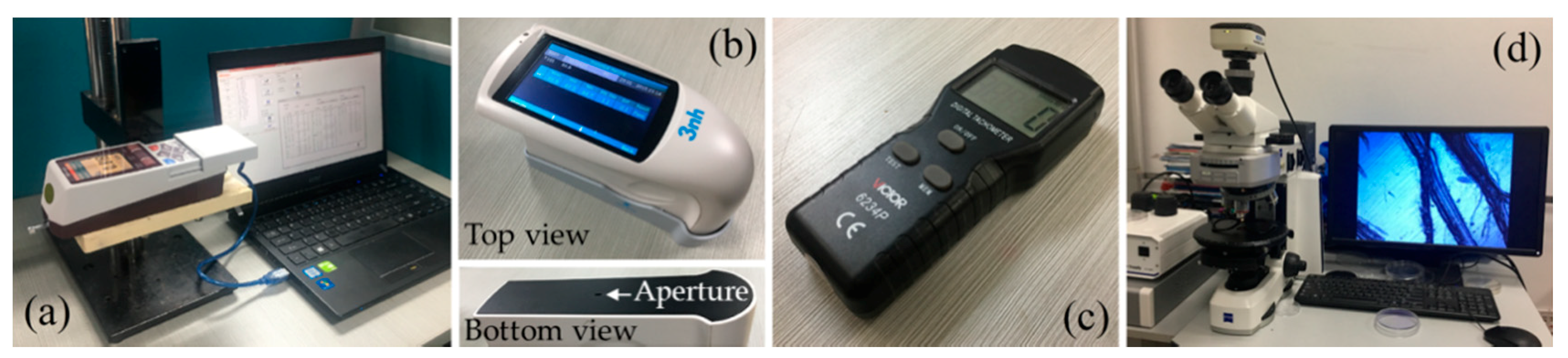
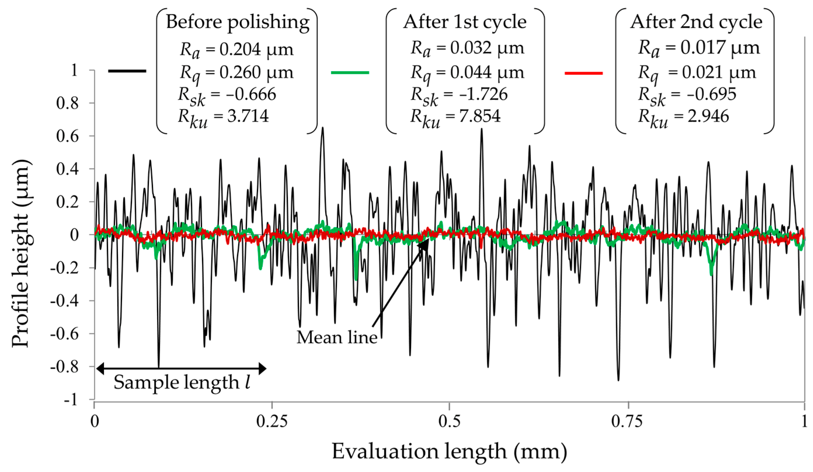
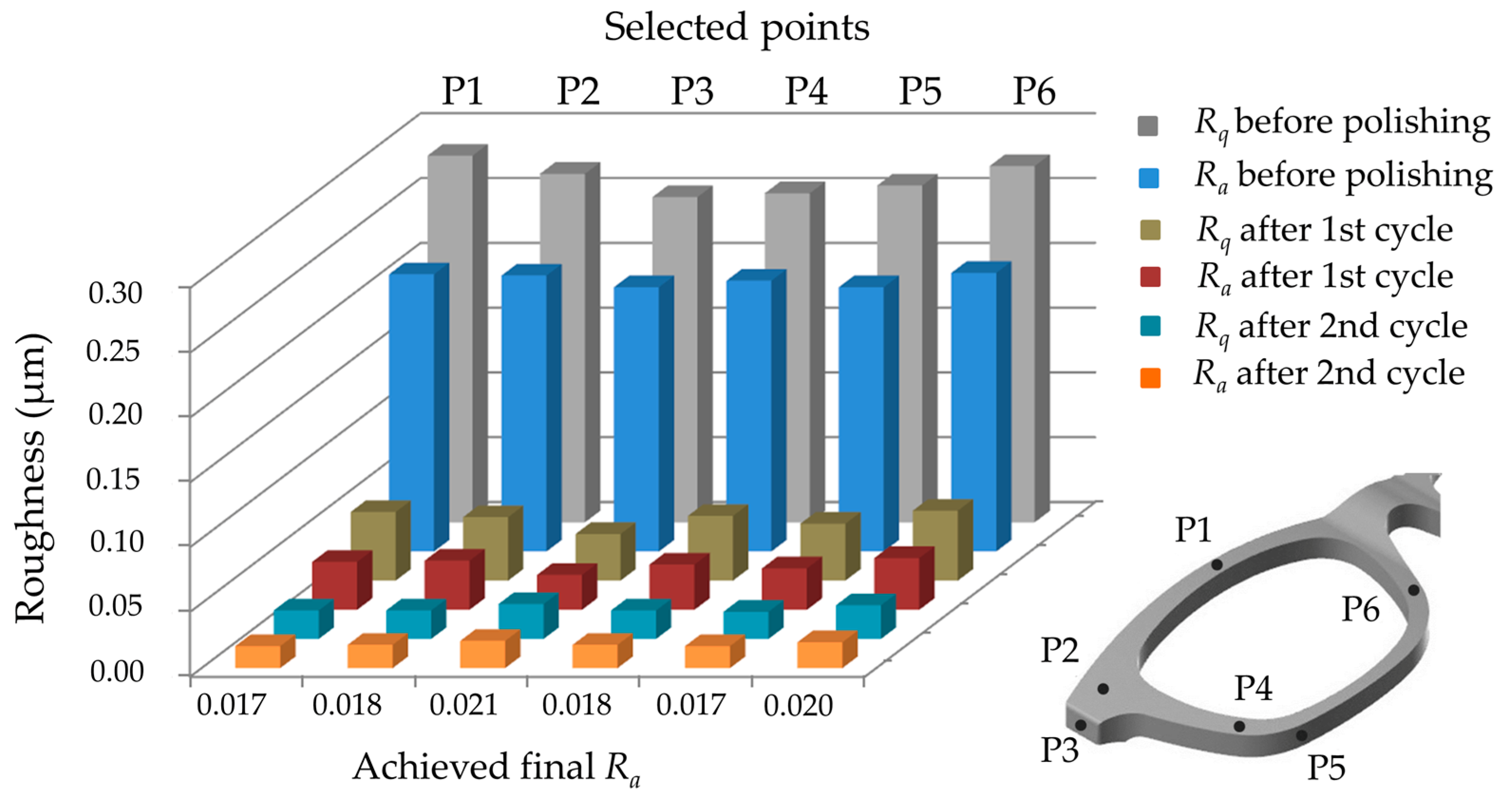
3.1. Surface Roughness

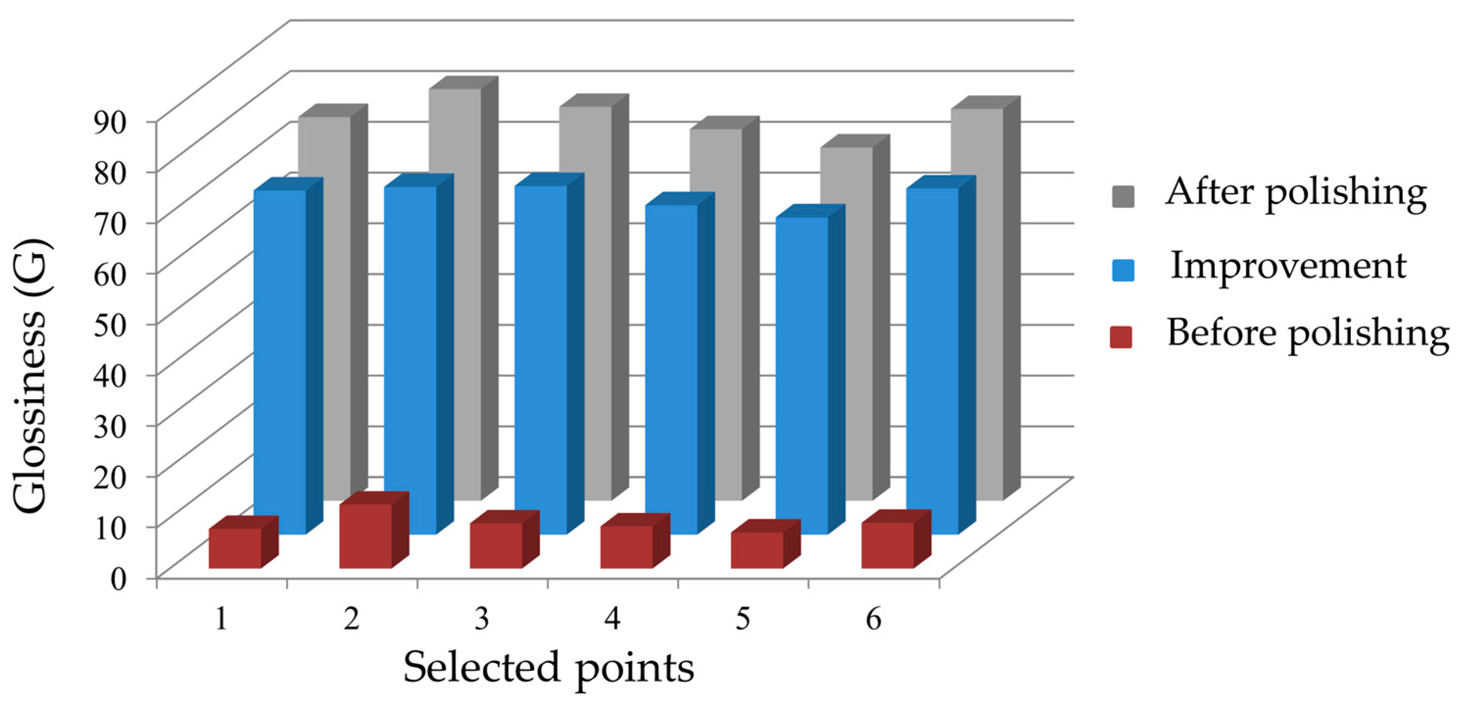
Arithmetic average roughness measurement is a well-established entity to evaluate the surface quality and it has been a crucial part of many theoretical and experimental studies. It is the average absolute deviation of the profile height y(x) from the mean line within the sample line. It is easy to measure and gives a general view of the height profile, however, it is not sensitive to small height variation and it does not give any information about wavelength. Conversely, the root mean square roughness ($R_q$) is the square root of the mean of the squared of roughness. It indicates the deviation of the distribution of the surface heights. Although $R_a$ is the most commonly used entity, the $R_q$ is more capable of large deviations from the mean line.

Figure 16 demonstrates the arithmetic average roughness height profile at a point on the part surface 1 of the eyeglass frame before and after polishing under 1 mm evaluation and 0.25 mm sample length. Besides the $R_a$ and $R_q$, skewness ($R_{sk}$) and kurtosis ($R_{ku}$) are also mentioned to understand the peaks and valleys formation during polishing steps. Before polishing, the surface has plenty of high peaks and deep valleys. After the 1st polishing cycle, this profile became negatively skewed ($R_{sk}$ = −1.726) because more high peaks are removed compared to the valleys. Moreover, fine grains of the polishing wax created shallow valleys that make the profile leptokurtic ($R_{ku}$ = 7.854). The second polishing cycle pushed it towards the normally distributed profile ($R_{ku}$ = 2.946), however still have fewer peaks ($R_{sk}$ = −0.695). The initial experimental analyses substantiate that the used of LCW and polishing wax can provide an average minimum $R_a$ of 0.017 µm. Further visualization of the surface topography of the eyeglass frame at the same point under the highly zoomed microscope is present in Figure 17 that shows the magnified photos taken at different polishing stages. Figure 17a shows the rough surface image before polishing with deep scratches. However, an effective polishing smoothed the surface as shown in Figure 17b with few shallow scratches left. The first polishing cycle improved 84% in the surface roughness approximately. The second polishing cycle further improved the surface as shown in Figure 17c. It gives gloss to the surface without any visible scratch.

By acknowledging the fact that the eyeglass frame is made of plastic (synthetic resin) and can easily deform its shape particularly at the edges if exposed to the tool for a longer time. Therefore, the higher SFPM and contact force are avoided. The minimum polishing force of 1 N for the $F_N$ is used throughout the experiments.

Table 1. Full factorial design of experiments (DOE) to find the economical polishing parameters at part surface one.

Exp. No.	Feed Rate (mm/s)	No. of Cycle	SFPM	Ra	$\mathit{P}\mathit{E}=\frac{{\mathit{A}\mathbf{\Delta }\mathit{R}}_{\mathit{a}}}{\mathit{T}}$	Exp. No.	Feed Rate (mm/s)	No. of Cycle	SFPM	Ra	$\mathit{P}\mathit{E}=\frac{{\mathit{A}\mathbf{\Delta }\mathit{R}}_{\mathit{a}}}{\mathit{T}}$
1	15	1	2950	0.032	13.06	16	45	2	3750	0.019	15.50
2	15	1	3750	0.020	13.97	17	45	3	2950	0.017	08.80
3	15	2	2950	0.017	07.07	18	45	3	3750	0.017	08.80
4	15	2	3750	0.017	07.07	19	60	1	2950	0.051	28.45
5	15	3	2950	0.015	04.03	20	60	1	3750	0.039	30.55
6	15	3	3750	0.016	04.01	21	60	2	2950	0.028	16.23
7	30	1	2950	0.033	22.59	22	60	2	3750	0.025	16.50
8	30	1	3750	0.023	23.86	23	60	3	2950	0.021	09.26
9	30	2	2950	0.017	12.30	24	60	3	3750	0.020	09.31
10	30	2	3750	0.017	12.30	25	75	1	2950	0.070	26.36
11	30	3	2950	0.015	06.97	26	75	1	3750	0.053	29.47
12	30	3	3750	0.016	06.94	27	75	2	2950	0.041	15.83
13	45	1	2950	0.038	27.97	28	75	2	3750	0.036	16.29
14	45	1	3750	0.029	29.44	29	75	3	2950	0.028	09.21
15	45	2	2950	0.020	15.43	30	75	3	3750	0.023	09.45

shows the complete experimental runs conducted at the part surface one ($S_1$) to find the optimized input polishing parameters for all the part surfaces. $R_a$ as an output of the polishing process was measured for different combinations of three input parameters. Every experiment was started with the average initial surface roughness of 0.214 µm. The polishing cycles were planned to achieve the target $R_a$ of 0.02 µm in a way that the first cycle was the workpiece motion against wheel rotation and in the later cycles, it would be in the direction of wheel rotation.

Figure 18 shows the $R_a$ curve against the feed rate for two different SFPM and three polishing cycles for the part surface one. A little disagreement in the graph from the trend line can be due to impurities in the polishing material. Increment in the feed rate increased the resultant roughness; however, with proper SFPM this rate could slowdown effectively. Suitable feed rate and SFPM could increase the polishing efficiency and achieve the desired surface quality in a short time. To find the highest PE by optimizing the polishing parameters, a graph between the $R_a$ and PE for all three polishing cycles with SFPM of 2950 and 3750 was plotted in Figure 19. It shows that the target roughness was achieved with all three polishing cycles at different feed rates. The maximum feed rates with a 10% safety margin to get the desired roughness in one, two, and three polishing cycles were 13 mm/s, 45 mm/s, and 54 mm/s respectively. However, the two polishing cycles with 3750 SFPM shows the maximum efficiency to get the target. Therefore, optimized polishing parameters (feed rate = 45 mm/s, no. of cycles = 2, and SFPM = 3750) from the graph were selected for polishing the all remaining 17 part surfaces of the eyeglass frame.

Table 2. Economical polishing parameters for each part surface of the eyeglass frame.

Polishing Cycle	Selected Tool	Polishing Material	SFPM (3750)		Feed Direction	Contact Force FN (N)	Feed Rate (mm/s)
			Wheel Diameter (mm)	Wheel Speed (rpm)
1	LCW	Dry finish Paste (P126)	152	2387	Against wheel rotation	1	45
2					In direction of wheel rotation

summarizes the optimized polishing parameters taken form the initial experimentation of the eyeglass frame polishing on surfaces $S_1$. It is supposed that all the part surfaces had approximately similar initial $R_a$ as $S_1$. It suggested two polishing cycles with SFPM of 3750 by LCW utilizing dry finish paste (P126 by Menzerna). Different combinations of wheel diameter and rotation speed were possible, which generated SFPM of 3750. A wheel with a 152 mm diameter and rotation speed 2387 rpm was adopted to polish.

Figure 20 demonstrates the surface roughness evolution for rough to mirror-like polishing in terms of $R_a$ and $R_q$ at all six selected points in different part surfaces. To minimize the chance of error, every measurement was repeated three times at the same point. It can be seen that the roughness dropped severely in the first polishing step, while it slowed down in the second step because of the feed direction in both steps. However, the second polishing cycle provided gloss to the surface. Before polishing, $R_a$ was ranging from 0.204 to 0.215 µm for six selected points that shows all part surfaces had nearly the same initial roughness. After the first polishing cycle, roughness reduced approximately 83% on average at the selected points. Average $R_a$ and $R_q$ were 0.0185 and 0.0233 µm respectively with the approximately 90% improvement in the surface height profile after two polishing steps. The major accomplishment of this robotic polishing was the resultant even surface quality in the freeform surface with economical parameters. $R_a$ values after polishing reflected this evenness with a very small variation from 0.018 to 0.021 µm.

3.2. Glossiness

Glossiness or specular reflection is another quality parameter for the polished surface that measures the visual appearance of the product. From Equation (11), glossiness (G) can be measured as the ratio of the specular reflectance of the target surface ($R_T$) to the specular reflectance of the polished glass ($R_o$) with a standard refractive index of 1.567 [35,36].

$$G=\frac{R_T}{R_o}\times 100\%$$

(11)

From the Fresnel equation, the specular reflectance (R) can be calculated as in Equation (12) [35]. It substantiates that incident angle i and refractive index n affect the spectral reflectance. Therefore, measurements at different angles were adopted in various standards. 20°, 60°, and 80° are mostly used angles in many measuring standards like ASTM D523 and DIN 67530. However, the 60° is the most adopted angle in many gloss meters as it is used in majority standards.

$$R=\frac{1}{R_S+R_P}=\frac{1}{2}\left[{\left(\frac{cosi-\sqrt{n^2-{sin}^{2}i}}{cosi+\sqrt{n^2-{sin}^{2}i}}\right)}^2+{\left(\frac{n^{2}cosi-\sqrt{n^2-{sin}^{2}i}}{n^{2}cosi+\sqrt{n^2-{sin}^{2}i}}\right)}^2\right]$$

(12)

Similarly, many studies have been established the relation between specular reflectance and surface roughness [35,37]. For example, H. E. Bennet and J. O. Porteus derived the following equation [38]:

$$R_S=R_{o}exp\left[-\frac{{\left(4\pi \sigma \right)}^2}{{\lambda }^2}\right]+R_o\frac{2^5{\pi }^4}{m^2}{\left(\frac{\sigma }{\lambda }\right)}^4{(\Delta \theta )}^2$$

(13)

Here, σ is the root mean square roughness, ∆θ is acceptance angle, m is the root mean square slope of the surface profile, and λ is a wavelength, which is assumed to be greater than the root mean square roughness. Surfaces with high roughness provide less gloss compared to the less rough surface.

Table 3. Measured glossiness at P3 using gloss meter.

S. No.	Mean Value	Max. Value	Min. Value	Standard. Deviation	Difference	Mean Glossiness
01	78.1	78.1	78.1	0.0	0.1	77.6
02	77.4	78.1	76.7	0.7	−0.6
03	77.7	78.3	76.7	0.7	−0.3
04	77.0	78.3	74.9	1.3	−1.0
05	77.6	80.0	74.9	1.7	−0.4

shows the glossiness comprehensive measurements at selected point P3 using gloss meter for best mean value with tolerance 10 G. A similar procedure was used throughout all sample surfaces. Five readings on the same points on every sample part surface were taken for the measurement.

Figure 21 presents the glossiness of all the selected six points before and after polishing. It also presents the improvement in the gloss after polishing. It shows the significant improvement in the glossiness of the part surfaces at different points between 62.5 and 68.7 G. It provided an average 88% improvement in glossiness in a short time just with two polishing cycles.

In manufacturing industries, machining economics is crucial to optimize the machine process. This optimization to get the target can be achieved by controlling the machining influencing variable parameters. Figure 22 shows the comparison in achieving the target roughness of 0.02 µm by three different no. of polishing cycles at their maximum efficiencies as in the PE vs. $R_a$ plot. This comparison demonstrates that the required surface quality can be attained by different parameters combinations; however, the correct selection of the parameters for tool path can save resources (such as time, energy, money, etc.). The minimum time taken by 1, 2, and 3 no. of polishing cycles were 136 s, 79 s and 184 s respectively. The best chosen 45 mm/s feed rate with two polishing cycles at 3750 SFPM achieves uniform roughness of target 0.02 µm in just 79 s. It is 42% and 57% less time compared to 136 s and 184 s respectively. Figure 23 shows the effect of robotic polishing on the selected polishing area of the final product.

4. Conclusions

This paper presented a robotic polishing method for complex curved surfaces based on a combination of tool path planning, force control, and optimized polishing parameters. From the above results and discussions, the following conclusions could be drawn:

(a) Robot polishing is a difficult task, in which the key considerations include: the surface area coverage, best-suited polishing parameters, the stable contact force, especially for complex surfaces, and the required surface quality (glossiness and uniformness). The presented method uses the divide-and-conquer strategy and is composed of four steps: workstation building, surface division, tool path generation, and tool path stitching. Based on the results of the tests on polishing eyeglass frames, this method was effective. It ensured the surface quality and avoided the robot running into singularities, joint limits, and jerks.

(b) The surface division is important. It decomposes a complex surface into a number of plain or simple curved surfaces. For each piece of surface, the robot could move smoothly and speedily. The main considerations in breaking a complex curved surface are edges of faces, variation in the orientation of surface normal vector, the robot joints limit, the curvature of the part surface, the size, and complexity of the surface.

(c) Three major research directions in robotic polishing are new tool design, path planning, and force control between tool and surface. However, the correct selection of the input process parameters could increase the efficiency exponentially and could be implemented with all three improvement techniques. The optimization of the parameters in this study was achieved by using full factorial DOE (30 experimental runs). The optimized input polishing parameters for the eyeglass frame were SFPM (3750), feed rate (45 mm/s), and no. of polishing cycles (2 cycles).

Based on the experimental results on polishing eyeglass frames, the presented method could achieve a high-quality surface with an average roughness of 0.0185 µm in 79 s. In addition, the entire surface was well covered and the average improvement in glossiness was 67 G, which was 88% improvement in just two polishing cycles. Moreover, all the scratches were eliminated successfully. It was believed that the presented method could be used on the shop floor directly.

References

1. Ohnishi, O.; Suzuki, H.; Uhlmann, E.; Schröer, N.; Sammler, C.; Spur, G.; Weismiller, M. Chapter 4—Grinding. In Handbook of Ceramics Grinding and Polishing; Marinescu, I.D., Doi, T., Uhlmann, E., Eds.; William Andrew Publishing: Boston, MA, USA, 2015; pp. 184–186. [Google Scholar]
2. Jakobsson, K.; Mikoczy, Z.; Skerfving, S. Deaths and tumours among workers grinding stainless steel: A follow up. Occup. Environ. Med. 1997, 54, 825–829. [Google Scholar] [CrossRef] [PubMed] [Green Version]
3. Beaulieu, H.J. Silica Dust and Concrete Grinding and Polishing: The Tragedy & the Beauty. 2008. Available online: http://www.dcpolish.com/concretegrindingdanger.html (accessed on 15 May 2019).
4. Grinding and Polishing Workers, Hand. Available online: https://www.bls.gov/oes/2018/may/oes519022.htm (accessed on 17 May 2019).
5. Tam, H.Y.; Lui, O.C.; Mok, A.C. Robotic Polishing of Free-Form Surfaces Using Scanning Paths. J. Mater. Process. Technol. 1999, 95, 191–200. [Google Scholar] [CrossRef]
6. Mizugaki, Y.; Sakamoto, M.; Sata, T. Fractal Path Generation for a Metal-Mold Polishing Robot System and Its Evaluation by the Operability. Cirp Ann. 1992, 41, 531–534. [Google Scholar] [CrossRef]
7. Rososhansky, M.; Xi, F.J. Coverage Based Tool-Path Planning for Automated Polishing Using Contact Mechanics Theory. J. Manuf. Syst. 2011, 30, 144–153. [Google Scholar] [CrossRef]
8. Kharidege, A.; Zhang, Y. A Practical Approach for Automated Polishing System of Free-Form Surface Path Generation Based on Industrial Arm Robot. Int. J. Adv. Manuf. Technol. 2017, 93, 3921–3934. [Google Scholar] [CrossRef]
9. Mohsin, I.; He, K.; Du, R. Robotic Polishing of Free-Form Surfaces with Controlled Force and Effective Path Planning. In Proceedings of the ASME IMECE Conference, Pittsburgh, PA, USA, 9–15 November 2018; pp. 1–9. [Google Scholar]
10. Oba, Y.; Kakinuma, Y. Tool Posture and Polishing Force Control on Unknown 3-Dimensional Curved Surface. In Proceedings of the ASME IMSEC Conference, Blackburg, VA, USA, 27 June–1 July 2016. [Google Scholar]
11. Mohsin, I.; He, K.; Cai, J.; Chen, H.; Du, R. Robotic polishing with force controlled end effector and multi-step path planning. In Proceedings of the ICIA, Macau, China, 18–20 July 2017; pp. 344–348. [Google Scholar]
12. Jinno, M.; Ozaki, F.; Yoshimi, T.; Tatsuno, K.; Takahashi, M.; Kanda, M.; Tamada, Y.; Nagataki, S. Development of a force controlled robot for grinding, chamfering and polishing. In Proceedings of the ICRA, Nagoya, Japan, 21–27 May 1995; pp. 1455–1460. [Google Scholar]
13. Wang, C.; Wang, Z.; Wang, Q.; Ke, X.; Zhong, B.; Guo, Y.; Xu, Q. Improved semirigid bonnet tool for high-efficiency polishing on large aspheric optics. Int. J. Adv. Manuf. Technol. 2016, 88, 1607–1617. [Google Scholar] [CrossRef]
14. Mohammad, A.E.; Hong, J.; Wang, D.; Guan, Y. Synergistic integrated design of an electrochemical mechanical polishing end-effector for robotic polishing applications. Robot. Comput. Integr. Manuf. 2019, 55, 65–75. [Google Scholar] [CrossRef]
15. Perez-Vidal, C.; Gracia, L.; Sanchez-Caballero, S.; Solanes, J.E.; Saccon, A.; Tornero, J. Design of a polishing tool for collaborative robotics using minimum viable product approach. Int. J. Comput. Integr. Manuf. 2019, 32, 848–857. [Google Scholar] [CrossRef]
16. Arunachalam, A.P.; Idapalapati, S.; Subbiah, S. Multi-criteria decision making techniques for compliant polishing tool selection. Int. J. Adv. Manuf. Technol. 2015, 79, 519–530. [Google Scholar] [CrossRef]
17. Zhan, J. An improved polishing method by force controlling and its application in aspheric surfaces ballonet polishing. Int. J. Adv. Manuf. Technol. 2013, 68, 2253–2260. [Google Scholar] [CrossRef]
18. Liu, Y.; Zhang, Y. Toward Welding Robot with Human Knowledge: A Remotely-Controlled Approach. IEEE Trans. Autom. Sci. Eng. 2015, 12, 769–774. [Google Scholar] [CrossRef]
19. Hertling, P.; Hog, L.; Larsen, R.; Perram, J.W.; Petersen, H.G. Task curve planning for painting robots. I. Process modeling and calibration. IEEE Trans. Robot. Autom. 1996, 12, 324–330. [Google Scholar] [CrossRef]
20. Yuan, P.; Wang, Q.; Shi, Z.; Wang, T.; Wang, C.; Chen, D.; Shen, L. A micro-adjusting attitude mechanism for autonomous drilling robot end-effector. Sci. China Inf. Sci. 2014, 57, 1–12. [Google Scholar] [CrossRef]
21. Gu, S.S.; Yang, C.Y.; Fu, Y.C.; Ding, W.F.; Huang, D.S. Grinding Force and Specific Energy in Plunge Grinding of 20crmnti with Monolayer Brazed Cbn Wheel. Mater. Sci. Forum 2014, 770, 34–38. [Google Scholar] [CrossRef]
22. Bifano, T.G.; Fawcett, S.C. Specific grinding energy as an in-process control variable for ductile-regime grinding. Precis. Eng. 1991, 13, 207–216. [Google Scholar] [CrossRef]
23. Linke, B.S.; Garretson, I.; Torner, F.; Seewig, J. Grinding Energy Modeling Based on Friction, Plowing, and Shearing. J. Manuf. Sci. Eng. 2017, 139, 1–11. [Google Scholar] [CrossRef] [Green Version]
24. Nagata, F.; Hase, T.; Haga, Z.; Omoto, M.; Watanabe, K. CAD/CAM-based position/force controller for a mold polishing robot. Mechatronics 2007, 17, 207–216. [Google Scholar] [CrossRef]
25. Mendes, N.; Neto, P. Indirect adaptive fuzzy control for industrial robots: A solution for contact applications. Expert Syst. Appl. 2015, 42, 8929–8935. [Google Scholar] [CrossRef]
26. Zhang, J.; Liu, G.; Zang, X.; Li, L. A hybrid passive/active force control scheme for robotic belt grinding system. In Proceedings of the ICMA, Harbin, China, 7–10 August 2016; pp. 737–742. [Google Scholar]
27. Craig, J.J. Introduction to Robotics Mechanics and Control, 3rd ed.; Horton, M.J., Ed.; Pearson Education, Inc. Pearson Prentice Hall: Upper Saddle River, NJ, USA, 2005; pp. 62–64, 148–151. [Google Scholar]
28. Zhao, Q.; Zhang, L.; Han, Y.; Fan, C. Polishing path generation for physical uniform coverage of the aspheric surface based on the Archimedes spiral in bonnet polishing. Proc. Inst. Mech. Eng. Part B J. Eng. Manuf. 2019, 233, 0954405419838655. [Google Scholar] [CrossRef]
29. Tsai, M.; Chang, J.-L.; Haung, J.-F. Development of an automatic mold polishing system. IEEE Trans. Autom. Sci. Eng. 2005, 2, 393–397. [Google Scholar] [CrossRef]
30. Tsai, M.J.; Huang, J.F. Efficient automatic polishing process with a new compliant abrasive tool. Int. J. Adv. Manuf. Technol. 2006, 30, 817–827. [Google Scholar] [CrossRef]
31. Han, G.; Sun, M. Compound control of the robotic polishing process basing on the assistant electromagnetic field. In Proceedings of the IEEE International Conference on Mechanical and Automation, Changchun, China, 9–12 August 2009; pp. 1551–1555. [Google Scholar]
32. Donelan, P.S. Singularity of robot manipulators. In Singularity Theory; Chéniot, D., Dutertre, N., Eds.; CIRM: Marseille, France, 2007; pp. 189–217. [Google Scholar]
33. Mehrban, M.; Kouravand, S.; Rezazadeh, G.; Donyavi, A. Application of Full Factorial Design Method in MEMS Capacitive Thermal Sensor Sensitivity. In Proceedings of the IEEE International Conference on Semiconductor Electronics, Kuala Lumpur, Malaysia, 29 October–1 December 2006; pp. 172–176. [Google Scholar]
34. Valizadeh, A.; Akbarzadeh, A.; Heravi, M.H.T. Effect of structural design parameters of a six-axis force/torque sensor using full factorial design. In Proceedings of the 3rd RSI International Conference on Robotics and Mechatronics (ICROM), Tehran, Iran, 7–9 October 2015; pp. 789–793. [Google Scholar]
35. Li, H.; Li, X.; Tian, C.; Yang, X.; Zhang, Y.; Liu, X.; Rong, Y. The simulation and experimental study of glossiness formation in belt sanding and polishing processes. Int. J. Adv. Manuf. Technol. 2016, 90, 199–209. [Google Scholar] [CrossRef]
36. Li, S.; Manabe, Y.; Chihara, K. Accurately estimating reflectance parameters for color and gloss reproduction. Comput. Vis. Image Underst. 2009, 113, 308–316. [Google Scholar] [CrossRef]
37. Yonehara, M.; Matsui, T.; Kihara, K.; Isono, H.; Kijima, A.; Sugibayashi, T. Experimental Relationships between Surface Roughness, Glossiness and Color of Chromatic Colored Metals. Mater. Trans. 2004, 45, 1027–1032. [Google Scholar] [CrossRef] [Green Version]
38. Bennett, H.E.; Porteus, J.O. Relation between Surface Roughness and Specular Reflectance at Normal Incidence. J. Opt. Soc. Am. 1961, 51, 123–129. [Google Scholar] [CrossRef]
Figure 1. The setup for the robotic polishing of the eyeglass frames.
Applsci 09 05489 g001
Figure 2. The flow chart of the proposed method for polishing the complex curved structures.
Applsci 09 05489 g002
Figure 3. Two different workstation building: (a) use tool as the end effector and (b) use workpiece as the end effector.
Applsci 09 05489 g003
Figure 4. Grinding/polishing force: (a) workpiece against polishing wheel and (b) tree diagram of the force components control.
Applsci 09 05489 g004
Figure 5. Different workpiece motions in polishing: (a) workpiece moving against wheel rotation direction and (b) workpiece moving in wheel rotation direction.
Applsci 09 05489 g005
Figure 6. Robot movement for the removal of residual forces in case of collision.
Applsci 09 05489 g006
Figure 7. The block diagram of the active contact flange (ACF).
Applsci 09 05489 g007
Figure 8. The illustration of the freeform surface using loose cotton wheel (LCW).
Applsci 09 05489 g008
Figure 9. Surface divisions of the eyeglass frame: (a) division into symmetric parts and faces and (b) complete division into part surfaces.
Applsci 09 05489 g009
Figure 10. Tool path patterns for plain and simple curved surfaces.
Applsci 09 05489 g010
Figure 11. Effect of the tool center point (TCP) position on flexible polishing tool (LCW) against the plain and curve surface: (a) curve surface with TCP at R; (b) curve surface with TCP at Rh and (c) plain surface with TCP at Rh.
Applsci 09 05489 g011
Figure 12. Toolpath of the four part surfaces of the eyeglass frame.
Applsci 09 05489 g012
Figure 13. Joints movement (degree) of all six joints of the robot during the polishing of the eyeglasses frame.
Applsci 09 05489 g013
Figure 14. Experimental setup for the robotic polishing of the eyeglass frame.
Applsci 09 05489 g014
Figure 15. Equipment used in experiments: (a) surface roughness tester (Mitutoyo, SJ-210); (b) gloss meter (NHG60M); (c) tachometer; and (d) microscope (ZEISS Axio Scope A1).
Applsci 09 05489 g015
Figure 16. Height profile of the surface of the eyeglass frame at P2.
Applsci 09 05489 g016
Figure 17. Magnified photos (200 µm) of the eyeglass frame surface at P2 in different stages: (a) before polishing, (b) after the first polishing cycle, and (c) after the second polishing cycle.
Applsci 09 05489 g017
Figure 18. Plot of roughness against feed rate for different surface feet per minute (SFPM) and polishing cycles.
Applsci 09 05489 g018
Figure 19. Plot of polishing efficiency against roughness for different SFPM and polishing cycles.
Applsci 09 05489 g019
Figure 20. Arithmetic and root mean roughness of all the six selected points at different polishing stages.
Applsci 09 05489 g020
Figure 21. Glossiness at all six selected points before and after polishing along with the improvement.
Applsci 09 05489 g021
Figure 22. Feed rate and time for selected polishing area on eyeglass frame at three different cycles.
Applsci 09 05489 g022
Figure 23. Eyeglass frame: (a) before polishing and (b) after robotic polishing.
Applsci 09 05489 g023