Abstract
This paper presents a procedure for an accurate and reliable stress analysis in a conical pick used in mining operations, aiming to improve their wear resistance. This is achieved by (1) establishment of a three-dimensional (3D) edge-based smoothed finite element method (ES-FEM), and algorithms of creating the smoothing domain for accurate solution in terms of stress and strain distributions; and (2) use of experimentally measured actual forces using a full-scale rotary cutting machine. In our 3D ES-FEM model, the physical domain for the pick is first discredited using linear triangular elements that can be generated easily for complicated geometries. The smoothing domains are then constructed based on edges of these elements in an automated fashion. In order to create the smoothing domains for the smoothed strain computation in the ES-FEM, an algorithm is presented for establishing connection between nodes, edges, faces, and elements. Each smoothing domain is bounded by a set of enclosed line-segments, besides, leading to a connectivity list for later effective computation. To show the effectiveness and accuracy of the strain energy and the displacement solution of ES-FEM, based on the actually measured forces from the laboratory rock cutting tests with a single pick, a comparison study is carried out against the standard finite element method (FEM). It can be concluded that ES-FEM has a higher convergence in energy norm and better accuracy than FEM using the same mesh from the comparison results. The 3D ES-FEM model solves the problem of the lower solution accuracy, caused by the poor quality of mesh, by using the standard FEM in solving the stress distribution of mining machinery parts, such as picks, and offers accurate and reliable solutions that are critical for improving the wear resistance of the pick for the mining industry.
1. Introduction
An imbalance in the excavation ratio has been a major obstacle affecting the safe and efficient production of coal. Especially, with the increase of rock hardness, various problems, such as pick wear and component failure, will arise, which often lead to lower efficiency, and even cause the machinery to not work. Therefore, if the mechanical properties of the cutter head for rock crushing and the wear mechanism of picks can be accurately assessed, the cutting performance of road headers will be greatly improved for higher efficiency industrial production. However, the working condition of a pick is often severe, complex, and dynamic in nature. Conical picks work usually under high impact and stress conditions, resulting in frequent failure. The failure modes include premature wear, carbide tip drop off, fracture, and normal wear [1,2,3,4,5,6,7]. In order to understand the cutting properties of a pick, researchers have carried out substantial experimental work on pick cutting force prediction. Experimental studies were performed to obtain the cutting performance parameters of conical picks, such as the pick force and wear influenced by cutting parameters and rock properties. Full-scale cutting tests in different types of sedimentary rocks, with bits having various degrees of wear, have been conducted to evaluate the influence of bit wear on cutting forces and specific energy. Studies have examined the relationship of the amount of wear represented by the size of wear flats at the tip of bits, cutting forces, and specific energy [5]. Liu also investigated the influence of pick cutting types, structures, and working angle parameters on pick wear, and the effect of wear on the pick cutting performance, by using an experimental apparatus to cut coal rock [6]. Bilgin et al. [8] carried out full-scale linear cutting tests, with different cutting depths and cut spacing, to study the conical pick performance on 22 different rock specimens, having compressive strength varying from 10 to 170 MPa. They found that the pick force and specific energy are positively correlated with rock properties, especially the uniaxial compressive strength and Brazilian tensile strength. Dewangan et al. [9,10,11] studied the wear mechanisms of conical picks in coal cutting by different testing methods. MacGregor compared the performance of buttons and conical picks based on data obtained from underground field trials, laboratory tests, and metallographic examinations. High cutting forces associated with worn picks have caused the increased vibration of a continuous miner [12]. In our work, for obtaining more accurate single-pick cutting test data, a large number of cutting tests were done on a full-scale rotary cutting machine, which is currently one of the most advanced single-pick rotary cutting machines to provide accurate cutting parameters for numerical simulation models.
In recent years, engineers and researchers have done large quantities of analysis on the forces imposed on a rock-cutting pick via simulations to study the wear of picks in the process of rock cutting. In numerical simulations, several computational methods have been widely used as efficient simulation tools to analyze the mechanical performance of picks and critical failure modes of rock fracture [13,14,15], like the finite element method (FEM), meshless methods, and so on. Du Xin and Ying Ming analyzed the effect of cutting pick stress with different cutting linear velocities using Pro/E (Pro/Engineer software) and the ANSYS (ANSYS is a large general finite element analysis software developed by ANSYS corporation) finite element method [16], in which the model was created and the loads were applied at the top of the cutting pick. Yan Pengfei studied the stress characteristics and failure mechanism of the cuttings under normal working condition, brazing loose condition, and tooth wear condition using ABAQUS which is a finite element analysis software [17,18]. In his study, the loads were applied on the conical surface, which was 4 mm away from the tip.
In order to obtain the good accuracy of the stress and strain solutions, these references used the hexahedral elements (H8), instead of the four-node tetrahedral element (T4), to mesh the problem domain. However, it is well known that H8 mesh cannot be automatically constructed and consumes more time for pre-process procedure. Besides, when the mesh is distorted, the result will become worse, and even in the standard FEM program it will break down because of the poor quality of the Jacobian matrix.
In consideration of these problems, smoothed finite element methods (S-FEMs) [19] have been developed using the strain smoothing technique, which has been developed based on G space theory [20,21] and weakened weak form (W2 form). It can overcome some disadvantages of FEM to obtain more convergent, stable, and accurate solutions in displacement and strain using T4 meshes. Besides, it was found that S-FEMs possess the excellent and distinctive properties, like softening effect, upper bounds, and ultra-accuracy [22,23,24].
When solving 3D problems, S-FEM can be classified as cell-based S-FEM [25,26], face-based S-FEM (FS-FEM) [27], node-based S-FEM (NS-FEM) [28], and edge-based S-FEM (ES-FEM) [29], according to the types of smoothing domains [30,31,32]. These different models have been employed to analyze mechanics problems, contact problems, heat transfer problems, and so on. In these previous works, it was found that ES-FEM using T4 meshes has several excellent properties, comparing with other S-FEMs and FEM, such as the nearly quadratic accuracy [33,34], which is very critical to solve the practical engineering problems. Because the structure and the working condition of conical picks are more complex, it is unrealistic to obtain higher accuracy relying on higher older elements. Nevertheless, ES-FEM can solve the problems easily, which can guarantee the nearly quadratic accuracy only using linear elements.
Thus, in this paper, for the analysis of the coal mining equipment, the ES-FEM is presented to reveal the stress and strain distributions of the conical pick, which can better master its working condition and effectively improve its wear resistance for engineers. T4 elements are employed as the background mesh and the edge-based smoothing domains are created based on it. Meanwhile, an algorithm is given for establishing connection between nodes, edges, faces, and elements. Then the smoothed strain-displacement matrices are constructed following the S-FEM theory for the smoothed stiffness matrices. Next the discrete linear algebraic system of equations is established like the procedure in FEM. What is more, the stress and strain distributions for conical picks are calculated, and the values of nodal displacement are calculated. Finally, the ES-FEM results for the conical pick with experimental measured forces were given and some comparisons with other S-FEM models and FEM were made.
2. Determination of the Pick Force
The cutter head operates with a composite motion, which includes rotating and swinging, and also through the conical tip of picks to break up the rocks. Due to the complex geological conditions in tunneling, it is very difficult to measure the cutting force imposed on the cutter head. Hence, the data obtained from the laboratory rock cutting tests with a single pick are usually used as the basis for calculating the forces of each cutter head pick. The prediction formulas of the pick forces obtained from the laboratory tests are more reasonable and reliable than those obtained in the theoretical and numerical simulation methods. In the paper, the cutting force acting on the pick is shown in Figure 1. The parameters present that d is the depth of cut, δ is the angle of attack, and n is the speed. FC is the cutting force, which is opposite to the direction of motion acting on the tip of the pick, and it is to separate the cuttings along the direction of the pick from the rock mass and forms a trough. FN is the normal force whose component force is perpendicular to the direction of motion of the coal rock, and it is to let the pick compress the rock and form the radiant point of the crack extension. Lastly, FS is the lateral force, from the normal force to the cutting direction according to the right-hand rule, and it is used to promote the rotation of the pick and forms a uniform wear.
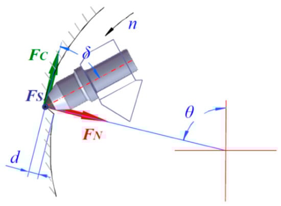
Figure 1.
Diagrammatic sketch of pick forces.
2.1. The Introduction of the Experimental Machine
The test is performed using a full-scale rotary cutting machine, which is currently one of the most advanced single-pick rotary cutting machines, at the National Engineering Laboratory of Coal Mining Machinery and Equipment in China. This machine consists of a test platform, a control system, a test system, and data analysis software. The structure of the test platform is shown in Figure 2. The device can sensitively monitor the cutting load, vibration, temperature, and dust amount during tests. The largest size of the sample rock that it can accommodate is 1400 × 800 × 600 mm. The rock is clamped with a special fixture to prevent it from moving under large impacts. Conical picks with wolfram carbide (WC) cemented carbide pick tip are used in the test, and the parameters are that the tip diameter is 25 mm, pick angle is 80°, external elongation of the pick is 80 mm, the handle width is 34 mm, and the handle length is 78 mm. In the whole test process, the cutting speed is 1.47 m/s, the cutting depth is 4 mm, the tool spacing is 12 mm, and the strike angle is 50°. The pick was used to cut the rock from the left to right end with a total of seventy cutting cycles under the same line spacing.
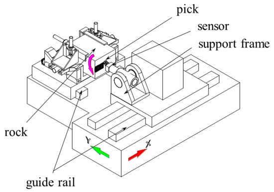
Figure 2.
Motion diagrammatic sketch of the rotary cutting machine.
2.2. The Mean Cutting Force of Conical Picks
Through the experiment, the normal force, the cutting force, and the lateral force from the experimental data are shown in Figure 3. It is easily found that the normal force is the largest among the components of the cutting load, the cutting force is the second, and the lateral force is the smallest. In this paper, the new pick was studied, so the first nine cutting test data were extracted to obtain the average force (Table 1). In our work, we set the normal force at 5.5 kN, the cutting force at 0.6 kN, and the lateral force at 0.002 kN.
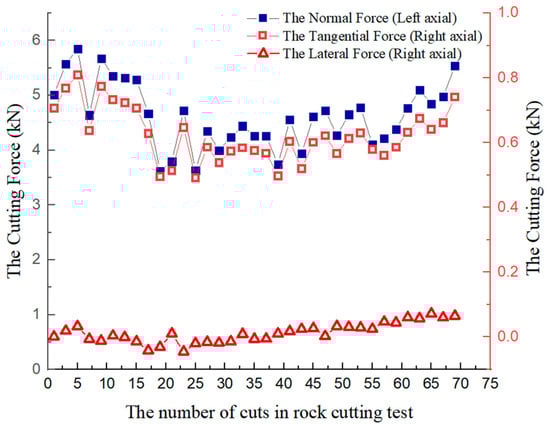
Figure 3.
The mean cutting force of conical picks varying with cuts.

Table 1.
The first nine cutting test data of the conical picks.
3. The Formulation of the Edge-Based Smoothed Finite Element Method (ES-FEM) for Conical Picks
3.1. Create the Edge-Based Smoothing Domains for Conical Picks
Before constructing the ES-FEM model, we uses the typical linear element T4 for 3D problems as the background mesh, which can automatically mesh and is very suitable for complex problem domains. Based on the T4 mesh, the edge-based smoothing domain can be created following the algorithm introduced below. In order to illustrate the process clearly, a simple ES smoothing domain is plotted in Figure 4 and the descriptions of elements and faces are listed in Table 2. Nodes n1, n2, n3, n4 made up the element 1 (e1); and nodes n1, n2, n3, n5 made up the element 2 (e2). Face1 (f1) contained nodes n1, n3, n4; Face2 (f2) contained nodes n1, n2, n3; Face3 (f3) contained nodes n1, n3, n5. In fact, ES smoothing domain relies on each edge so the number of smoothing domains equals the number of edges in the background. The smoothed domain will adopt the edges on the element as the indexes. Take the element in the Figure 4, for example, there are two elements e1 and e2. We will discuss how to build the smoothing domain of edge n1n3. The edge of n1n3 is an internal edge which is related to the different elements. Let us focus on the element e1, because the process is the same as that in the element e2. In this element, the edge locates on the faces f1, f2, and f3. Then connect the center of one face, the centroid of this element, and one vertex of the edge to form a surface-segment of the smoothing domain. Repeat the process and obtain six-surface segments for one element, n3cf1ce1, n1cf1ce1, n3cf2ce1, n1cf2ce1. Similarly, we can build other six-surface segments for the element e2. It is clearly seen that the 3D-edge-based smoothed domain is enclosed by these surfaces. Hence, the ID of the smoothing domain is the same as the ID of the edge, which is surrounded by the smoothing domain. In Figure 4, one T4 element is separated by six smoothing domains according to the edges of this element.
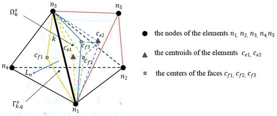
Figure 4.
3D-edge-based smoothing domains.
Table 2.
The details of the grid in Figure 4.
Through the above introduction, the constructing algorithm needs the connectivity of element, face, edge, and node. Therefore, for creating a smoothing domain quickly, we first need to get the connectivity of nodes separately with elements, faces, and edges; the connectivity of edges separately with elements, faces, and nodes; the connectivity of faces separately with elements, edges, and nodes; and the connectivity of elements separately with faces, edges, and nodes.
3.2. Construct the Smoothed Strain Field of ES-FEM
In an ES-FEM model, each of the smoothing domains , in general consist of sub-smoothing domain , which is a part of the elements where the corresponding edge locates.
The smoothed strain field for one smoothing domain can be obtained by boundary flux as follows:
where is the boundary of the qth sub-smoothing domain of smoothing domain , is the boundary of the smoothing domain , , is the volume of the smoothing domain , which has the form of , and is the volume of the jth tetrahedral element around edge . is the number of the sub-smoothing domain. is the displacement matrix, which has the form of
where the displacement matrix of all nodes in ES-FEM and is the shape function matrix. is the matrix of components of the outward normal vector on the boundary , hence the form as:
3.3. Construct the ES Smoothed Strain-Displacement Matrix
Substituting Equation (2) into Equation (1), the smoothed strain is:
where is the global “smoothed strain-displacement” matrix, which is due to the shape function matrix . For ES-FEM using the four-node tetrahedron element, as shown Figure 4, the set of nodes are {n1, n2, n3, n4, n5} for edge k. The smoothed strain-displacement matrix is evaluated using:
where
Therefore, for the internal edge of four-node tetrahedron element, is a matrix of 6 × 15, for the border edge, is a 6 × 12 matrix. Besides, is a vector containing 12 elements.
The Equation (6) can be further simplified to a summation form by using the Gauss quadrature technique:
where is the total number of boundary segment and is the Gauss point of boundary segment of ,whose area and outward unit normally are donated as and , respectively.
Thus, can be given in detail as follows:
The general formulation for computing the smoothed stiffness matrix is
with entries
where c is the matrix of material constants.
4. Results
In the section, in order to illustrate the efficiency and accuracy of the present ES-FEM algorithm for conical pick problems, the numerical results of EF-FEM are listed and are compared with the solutions of other S-FEM models and FEM in stress, strain energy, and displacement.
The geometrical parameters of the practical conical pick used in our experiment are given in Figure 5. The material parameters in the experiment used are: and . At the same time, the normal force of , the cutting force of , and the lateral force of are imposed on the top surface of the conical pick, and the force area is three-quarters of the top area shown in Figure 6. First, the numbers and area of the forced elements are obtained based on the ES-FEM mesh; and then the forces of one element are imposed on three nodes through the face normal algorithm. Besides, we fully fix the bottom of the conical pick.
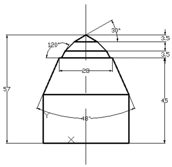
Figure 5.
Geometrical model of the conical pick.
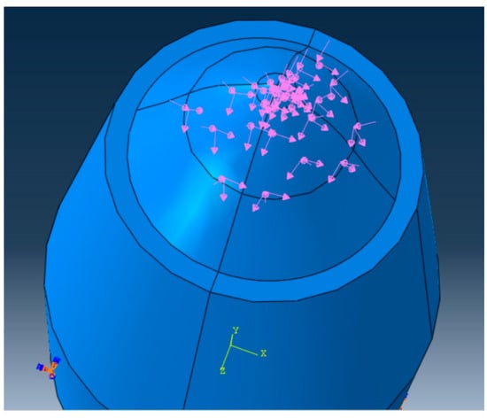
Figure 6.
The forces area and position.
For practical problems, it is very difficult to find the analytical solution. Hence, we calculate the reference solutions of the problem using the standard FEM with the mesh of 65,686 T4 elements, and 197,058 degrees of freedom.
In Figure 7a, the conical pick is divided by tetrahedron elements as the background mesh. We use the connectivity of the background mesh listed above the tables and the algorithm mentioned in Section 3.1 to create an ES mesh for our numerical simulation (Figure 7b). From this figure, we can observe the smoothing domains are surrounding the edges in the background mesh. Seven background meshes are applied to different methods such as FEM, ES-FEM, FS-FEM, NS-FEM, which have the same numbers of nodes, elements, and degrees of freedom. The detailed information of these seven meshes is shown in Table 3.
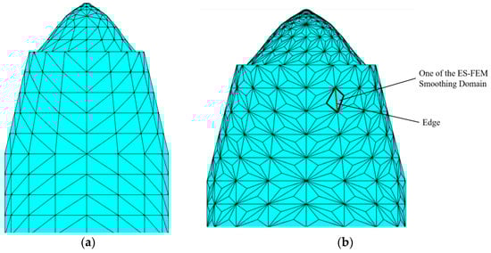
Figure 7.
(a) The background mesh and (b) the ES-FEM mesh of conical pick.
Table 3.
Description of the seven meshes.
4.1. The Stress Solutions
Von-Mises stress, which is the fourth strength theory, can clearly describe the change of a result in the whole model through using stress contours to represent the stress distribution, and makes sure designers can quickly determine the most dangerous area in the model. Thus, Von-Mises stress is used to describe stress distribution in post-processing of mature FEM software. In order to verify the validity and accuracy of our method, we compared the Von-Mises stress value of ES-FEM with the reference value and FEM analysis results. Von-Mises stress is computed using the stress components in the form of:
Figure 8 is the reference value of Von-Mises stress using the standard FEM with 197,058 degrees of freedom. Then we plot the distribution of von-Mises stress using the present ES-FEM and FEM with the mesh having 6413 T4 elements in Figure 9. It is easily seen that the Von-Mises stress distributions of the ES-FEM model are similar to that of FEM.
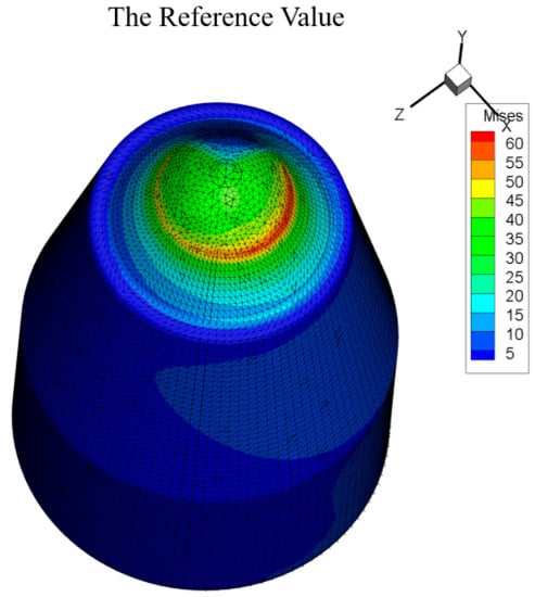
Figure 8.
The reference value of Von-Mises stress .
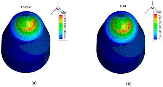
Figure 9.
(a) The Von-Mises stress distribution using ES-FEM; (b) The Von-Mises stress distribution using FEM.
Further, we compares the maximum Von-Mises stress of ES-FEM with FEM, NS-FEM, and FS-FEM against the degrees of freedom in Figure 10. It is obviously observed that FEM is the stiffest, and ES-FEM is softened by the smoothing technique. Besides, NS-FEM still keeps the property of upper bounds. Among the results of S-FEMs and the FEM, the ES-FEM solution is the closest one to the reference solution.
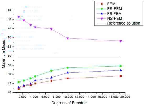
Figure 10.
The maximum Von-Mises stress obtained using different methods for the conical picks using the same triangular meshes.
Next, the distribution of Von-Mises stress along the generator of the tip which includes the max Von-Mises stress using different methods for the conical pick are computed and shown in Figure 11. We first find that the maximum von-Mises in the Figure 11 was about 7.5 mm away from the apex of conical pick, and the von-Mises would be steadily reducing with the distance increasing from the apex. In addition, it is shown that the ES-FEM Von-Mises are closer to the reference solutions than that of FEM. It was further proof that our ES-FEM for the practical conical pick is more accurate and efficient among other S-FEM methods and FEM.
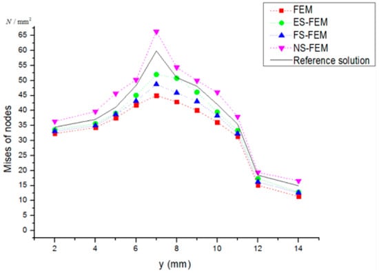
Figure 11.
The distribution of Von-Mises stress along the generator of the tip using different methods for the conical pick.
4.2. The Strain Energy Solutions
In the section, we studied the performance of the ES-FEM on the strain energy for this practical problem. First, we calculated the reference solution of strain energy using the finer mesh mentioned above, which is 2.4240 . Then, the numerical results of strain energy using different methods are presented in Table 4. The error of strain energy obtained using ES-FEM is smallest no matter which mesh is used. The according convergence curves of strain energy is plotted in Figure 12 against the degrees of freedom (DOFs). It can be found that the strain energy of ES-FEM are just a little bigger than the reference solution and quickly converge to it with the increase of DOFs. In contrast, the strain energy solution of FEM is much lower than the reference solution and it converges very slowly. It is noted that, although the ES-FEM solution fluctuates a little bit when using the coarse meshes, the value is more close to the reference solution than other methods. Besides, it is observed that the upper bounds of NS-FEM and the lower bounds of FEM still remain the same in this simulation.
Table 4.
The error of strain energy obtained using different methods compared to the reference solution (%).
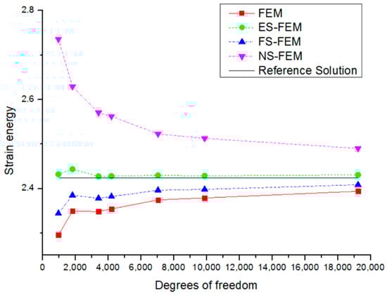
Figure 12.
Convergence of the strain energy solution for the conical picks.
Next, in order to verify the accuracy and validity, the error norm of the strain energy of ES-FEM was calculated and compared with that of FEM, NS-FEM, and FS-FEM models. Errors of these numerical methods are analyzed using energy norms. The error norm of strain energy is calculated by:
where is the reference solution for the strain energy, and is the numerical solution for the strain energy using a numerical model. Table 5 lists seven sets of data calculated using different methods for seven meshes. It is shown that the error of ES-FEM is about 0.217 against 0.534 of FEM, which illustrates again that ES-FEM stands out clearly.
Table 5.
Error in strain energy norm obtained using different methods for the conical picks.
4.3. The Nodes Displacement Solutions
In this part, we will examine the displacement solution for the conical pick. The reference value of nodes’ displacements along y-axis and z-axis are plotted in Figure 13 and we draw the approximate displacement solutions along the y-axis and z-axis using ES-FEM in Figure 14. From these figures it is distinctly observed that the displacement solutions of ES-FEM are reasonable and accurate.
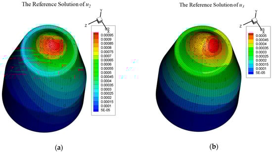
Figure 13.
The reference value of nodes’ displacements along (a) the y-axis and (b) z-axis .
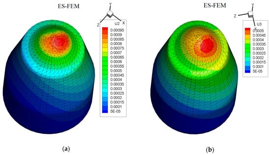
Figure 14.
The approximate displacement solutions along (a) the y-axis and (b) z-axis using ES-FEM.
Table 6 shows the comparison of displacements of ES-FEM with FEM, NS-FEM, and FS-FEM. Figure 15 is plotted by the distance from the tip of the conical pick on the horizontal axis and the node’s displacement on the vertical. The comparison is fair and rigorous as long as the same distribution of nodes is used. Overall, the displacements of ES-FEM are closer to the reference solutions than those of FEM. This also verifies that, regardless of strain and displacement, ES-FEM is the most accurate and stable method compared with FEM and other S-FEMs.
Table 6.
The displacement along the tip using FEM, ES-FEM, FS-FEM, and NS-FEM for the conical pick (10−3 mm).
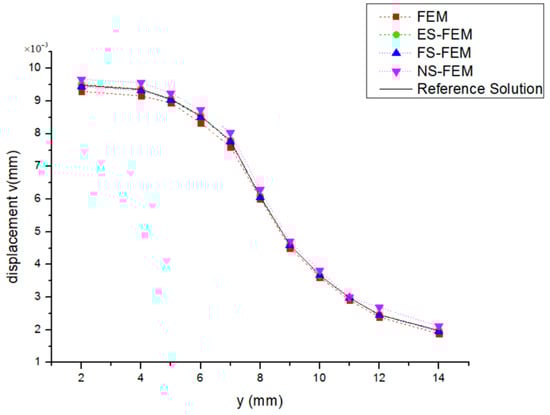
Figure 15.
The distribution of displacement v along the tip using different methods for the conical pick.
In order to further verify the accuracy and stability, the error of displacement of the ES-FEM model was conducted. Displacement errors and convergence rates of these numerical methods are analyzed using displacement norms. The displacement norm is defined as:
where is the reference solution of the displacements, and is the numerical solution of the displacements using a numerical model. Table 7 compares the solution errors in the displacement norm obtained using FEM, ES-FEM, FS-FEM, and NS-FEM. The error of ES-FEM is about 0.216 times that of FEM, 0.8 times that of FS-FEM, and 0.213 times that of NS-FEM. In terms of convergence rate, compared with other methods, the ES-FEM performs the best.
Table 7.
Error in the displacement norm for the ES-FEM solution in comparison with those of other methods for the cemented carbide picks using the same distribution of nodes.
4.4. The Computational Efficiency of Solutions
In the final part, we discuss the computational efficiency of the methods for this example. The efficiency is estimated using the following formulation:
where is the strain energy norm error of different methods compared with FEM, and represents CPU time compared with FEM. Table 8 and Table 9 list the strain energy norm error and CPU time obtained using four methods with mesh 4 and mesh 5. It is easily found that the solution error of ES-FEM is the smallest even though the CPU time is one of the highest. Taking the two facts into consideration, the computational efficiency objectively describes the performance of different numerical methods. Hence, ES-FEM, whose computational efficiency is about 2.88 times that of FEM, is the most efficient one. Similarly, the computational efficiency of FS-FEM has been improved in comparison with FEM. Thus, the computational efficiency of ES-FEM and FS-FEM can be significantly improved when CPU time is taken into account.
Table 8.
Estimated computational efficiency of four methods, measured in strain energy norm error using mesh 4.
Table 9.
Estimated computational efficiency of four methods, measured in strain energy norm error using mesh 5.
5. Conclusions
In the paper, the efficient and ultra-accurate ES-FEM is used to simulate the cutting process of conical picks. Through analyzing the cutting characteristics of a conical pick, the normal force, the cutting force, and the lateral force are obtained from the experimental data using a full-scale rotary cutting machine as the boundary conditions in our simulation. Firstly, we present an efficient algorithm for creating edge-based smoothing domains, which generates the twelve connectivity lists, including the connectivity of face–node, face–edge, face–element, node–face, edge–face, element–face, edge–node, edge–element, element–edge, node–edge, node–element, and element–node. Then the gradient smoothing technique is employed to construct the smoothed strain gradient and displacement gradient fields. Next, the smoothed system equations are set up following the theory of S-FEM. Finally, displacement, strain energy, and stress are calculated using the ES-FEM for the conical pick. At the same time, various comparisons between ES-FEM and other methods are made to demonstrate the accuracy and effectiveness of the ES-FEM model. The concluding remark was drawn as follows:
- The procedure of the ES smoothing domain presented in this paper is very easy and performs very well for the complex structured parts of coal mining machines.
- The present method showed a better accuracy and convergence rate than FEM for this practical problem, which illustrate S-FEM is suitable for practical engineering problems.
Author Contributions
Conceptualization, G.L.; test analysis, Q.Z.; numerical simulation and writing, Q.F.
Funding
This work supported by Shanxi Provincial Natural Science Foundation of China under Grant 201801D221215. This work supported by Shanxi Provincial Natural Science Foundation of China under Grant 201901D211120. This work supported by China Scholarship Council, File No.201708140187.
Conflicts of Interest
The authors declare no conflict of interest.
References
- Park, J.Y.; Kang, H.; Lee, J.W.; Kim, J.-H.; Oh, J.-Y.; Cho, J.-W. A study on rock cutting efficiency and structural stability of a point attack pick cutter by lab-scale linear cutting machine testing and finite element analysis. Int. J. Rock Mech. Min. Sci. 2018, 103, 215–229. [Google Scholar] [CrossRef]
- Rojek, J.; Onate, E.; Labra, C.; Kargl, H. Discrete element simulation of rock cutting. Int. J. Rock Mech. Min. Sci. 2011, 48, 996–1010. [Google Scholar] [CrossRef]
- Van Wyk, G.; Els, D.N.J.; Akdogan, G.; Bradshaw, S.M.; Sacks, N. Discrete element simulation of tribiological interactions in rock cutting. Int. J. Rock Mech. Min. Sci. 2014, 65, 8–19. [Google Scholar] [CrossRef]
- Li, X.; Wang, S.; Ge, S.; Malekian, R.; Li, Z. Numerical simulation of rock fragmentation during cutting by conical picks under confining pressure. Comput. Rendus Méc. 2017, 345, 890–902. [Google Scholar] [CrossRef]
- Dogruoz, C.; Bolukbasi, N.; Rostami, J.; Acar, C. An experimental study of cutting performances of worn picks. Rock Mech. Rock Eng. 2016, 49, 213–224. [Google Scholar] [CrossRef]
- Liu, S.; Ji, H.; Liu, X.; Jiang, H. Experimental research on wear of conical pick interacting with coal-rock. Eng. Fail. Anal. 2017, 74, 172–187. [Google Scholar] [CrossRef]
- Amri, M.; Pelfrene, G. Numerical and analytical study of rate effects on drilling forces under Bottom hole pressure. Int. J. Rock Mech. Min. Sci. 2018, 110, 189–198. [Google Scholar] [CrossRef]
- Bilgin, N.; Copur, H. Dominant rock properties affecting the performance of conical picks and the comparison of some experimental and theoretical results. Int. J. Rock Mech. Min. Sci. 2006, 43, 139–156. [Google Scholar] [CrossRef]
- Dewangan, S.; Chattopadhyaya, S.; Hloch, S. Wear Assessment of Conical Pick used in Coal Cutting Operation. Rock Mech. Rock Eng. 2015, 48, 2129–2139. [Google Scholar] [CrossRef]
- Dewangan, S.; Chattopadhyaya, S. Characterization of Wear Mechanisms in Distorted Conical Picks after Coal Cutting. Rock Mech. Rock Eng. 2016, 49, 225–242. [Google Scholar] [CrossRef]
- Dewangan, S.; Chattopadhyaya, S. Performance Analysis of Two Different Conical Picks Used in Linear Cutting Operation of Coal. Arab. J. Sci. Eng. 2016, 41, 249–265. [Google Scholar] [CrossRef]
- MacGregor, I.M.; Baker, R.H.; Luyckx, S.B. A comparison between the wear of continuous miner button picks and the wear of pointed picks used in South African collieries. Min. Sci. Technol. 1990, 11, 213–222. [Google Scholar] [CrossRef]
- Huang, J.; Zhang, Y.M.; Zhu, L.; Wang, T. Numerical simulation of rock cutting in deep mining conditions. Int. J. Rock Mech. Min. Sci. 2016, 84, 80–86. [Google Scholar] [CrossRef]
- de Li, R.; Li, J.N.; Wang, S.F. Study on Numerical Simulation and Wear Mechanism of Cutting Pick. Coal Mine Mach. 2016, 37, 57–60. [Google Scholar]
- Jaime, M.C.; Zhou, Y.; Lin, J.S.; Gamwo, I.K. Finite element modeling of rock cutting and its fragmentation process. Int. J. Rock Mech. Min. Sci. 2015, 80, 137–146. [Google Scholar] [CrossRef]
- Du, X.; Ying, M.; Han, B. Analysis of Cutting Pick Stress with Different Cutting Linear Velocity. Coal Mine Mach. 2013, 34, 89–92. [Google Scholar]
- Yan, P.F. Failure Form and Strength Analysis of Picking of Shearer. Coal Technol. 2017, 36, 261–263. [Google Scholar]
- Gao, Y.; Zhou, T. Numerical simulation and analysis for bit impact on pyrites based on 3D FEM-SPH conversion algorithm. J. China Coal Soc. 2017, 42, 568–572. [Google Scholar]
- Liu, G.R. On Future computational methods for exascale computers. Express Bull. Int. Assoc. Comput. Mech. 2011, 30, 8–10. [Google Scholar]
- Liu, G.R.; Trung, N.T. Smoothed Finite Element Methods; CRC Press: Boca Raton, FL, USA, 2010; Volume 691. [Google Scholar]
- Liu, G.R.; Zhang, G.Y. A normed G space and weakened formulation of a cell-based smoothed point interpolation method. Int. J. Comput. Methods 2009, 6, 147–179. [Google Scholar] [CrossRef]
- Liu, G.R.; Zhang, G.Y. The Smoothed Point Interpolation Methods—G Space Theory and Weakened Weak Forms, 1st ed.; World Scientific: New Jersey, USA, 2013. [Google Scholar]
- Liu, G.R. A G space theory and a weakened weak (W2) form for a unified formulation of compatible and incompatible methods: Part II: Applications to solid mechanics problems. Int. J. Number Methods Eng. 2009, 81, 1127–1156. [Google Scholar] [CrossRef]
- Chen, J.; Wu, C.; Yoon, S.; You, Y. A stabilized conforming nodal integration for Galerkin mesh-free methods. Int. J. Number Methods Eng. 2001, 50, 435–466. [Google Scholar] [CrossRef]
- Liu, G.R. A generalized gradient smoothing technique and the smoothed bilinear form for galkerin formulation of a wide class of computational methods. Int. J. Comput. Methods 2008, 5, 199–236. [Google Scholar] [CrossRef]
- Liu, G.R.; Dai, K.Y.; Nguyen, T.T. A smoothed finite element method for mechanics problems. Comput. Mech. 2006, 39, 859–877. [Google Scholar] [CrossRef]
- Liu, G.R.; Nguyen, T.T.; Dai, K.Y.; Lam, K.Y. Theoretical aspects of the smoothed finite element method (SFEM). Int. J. Number Methods Eng. 2007, 71, 902–930. [Google Scholar] [CrossRef]
- Nguyen Thoi, T.; Liu, G.R.; Lam, K.Y.; Zhang, G.Y. A face-based smoothed finite element method (FS-FEM) for 3D linear and geometrically non-linear solid mechanics problems using4-node tetrahedral elements. Int. J. Number Methods Eng. 2009, 78, 324–353. [Google Scholar] [CrossRef]
- Liu, G.R.; Nguyen-Thoi, T.; Nguyen-Xuan, H.; Lam, K.Y. A node-based smoothed finite element method (NS FEM) for upper bound solutions to solid mechanics problems. Comput. Struct. 2009, 87, 14–26. [Google Scholar] [CrossRef]
- Liu, G.R.; Nguyen-Thoi, T.; Lam, K.Y. A novel alpha finite element method (αFEM) for exact solution to mechanics problems using triangular and tetrahedral elements. Comput. Methods Appl. Mech. Eng. 2008, 197, 3883–3897. [Google Scholar] [CrossRef]
- Zhang, Z.; Liu, G.R. Temporal stabilization of the node-based smoothed finite element method and solution bound of linear electrostatics and vibration problems. Comput. Mech. 2009, 46, 229–246. [Google Scholar] [CrossRef]
- Niu, R.P.; Liu, G.R.; Yue, J.H. Development of a Software Package of Smoothed Finite Element Method (S-FEM) for Solid Mechanics Problems. Int. J. Comput. Methods 2018, 3, 1845004. [Google Scholar] [CrossRef]
- Zhang, Z.; Liu, G.R. Solution bound and nearly exact solution on linear solid mechanics problems based on the smoothed FEM concept. Eng. Anal. Bound. Elem. 2014, 42, 99–114. [Google Scholar] [CrossRef]
- Yao, J.; Liu, G.R.; Narmoneva, D.A.; Hinton, R.B.; Zhang, Z.-Q. Immersed smoothed finite element method for fluid-structure interaction simulation of aortic valves. Comput. Mech. 2012, 50, 789–804. [Google Scholar] [CrossRef]
© 2019 by the authors. Licensee MDPI, Basel, Switzerland. This article is an open access article distributed under the terms and conditions of the Creative Commons Attribution (CC BY) license (http://creativecommons.org/licenses/by/4.0/).