Landslide Susceptibility Mapping for Austria Using Geons and Optimization with the Dempster-Shafer Theory

 ,
, 
 ,
,  and
and 
Abstract
1. Introduction
2. Study Area
3. Materials and Methods
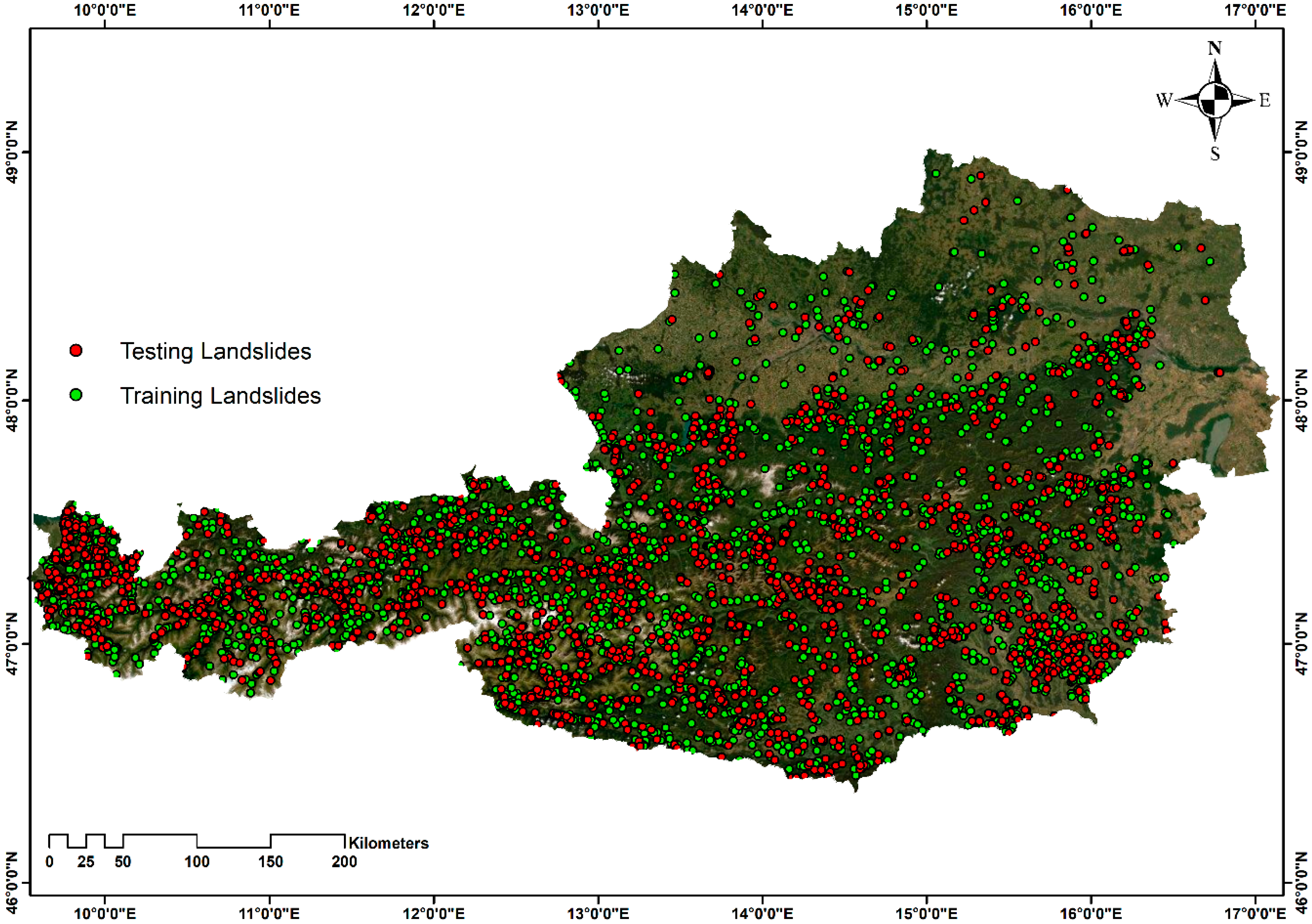
3.1. Landslide Inventory Data
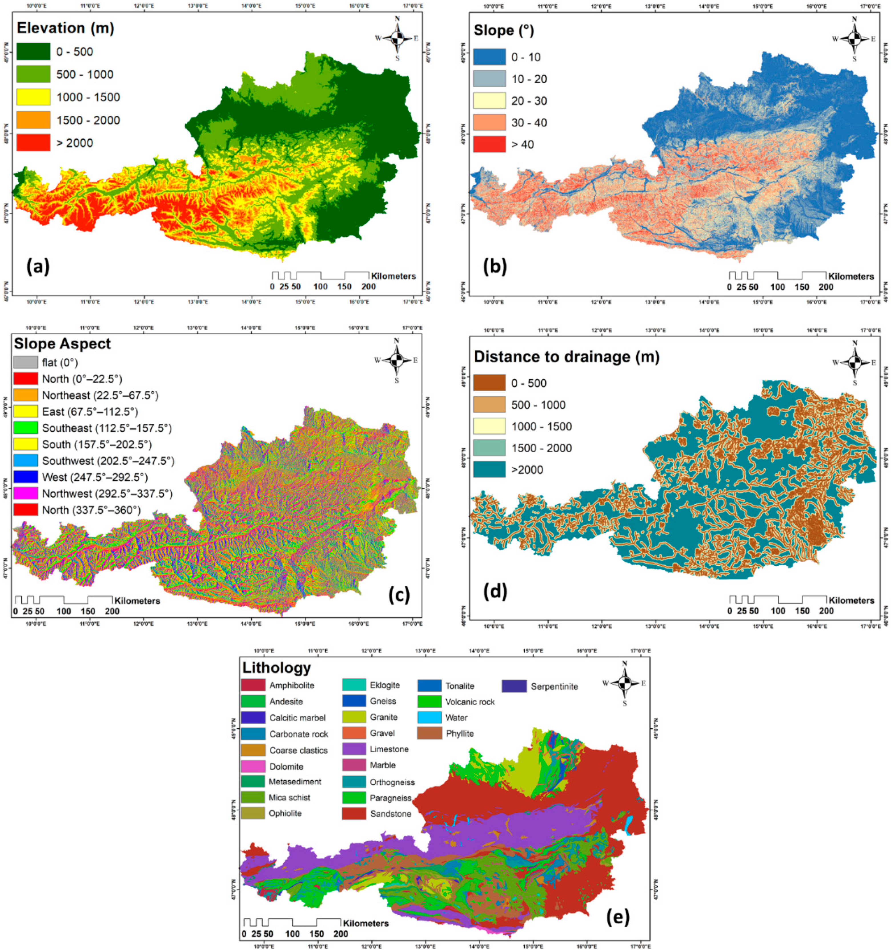
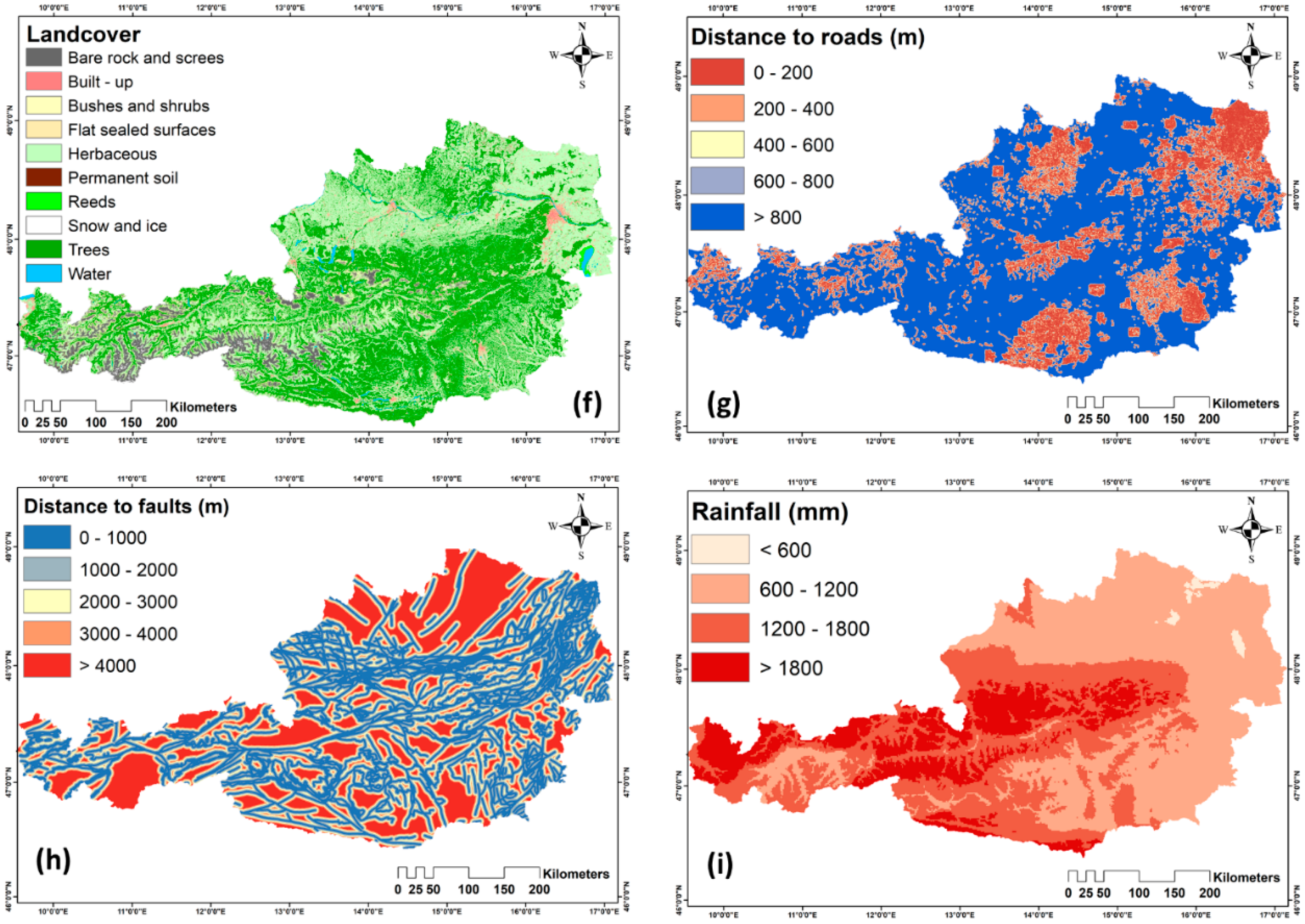
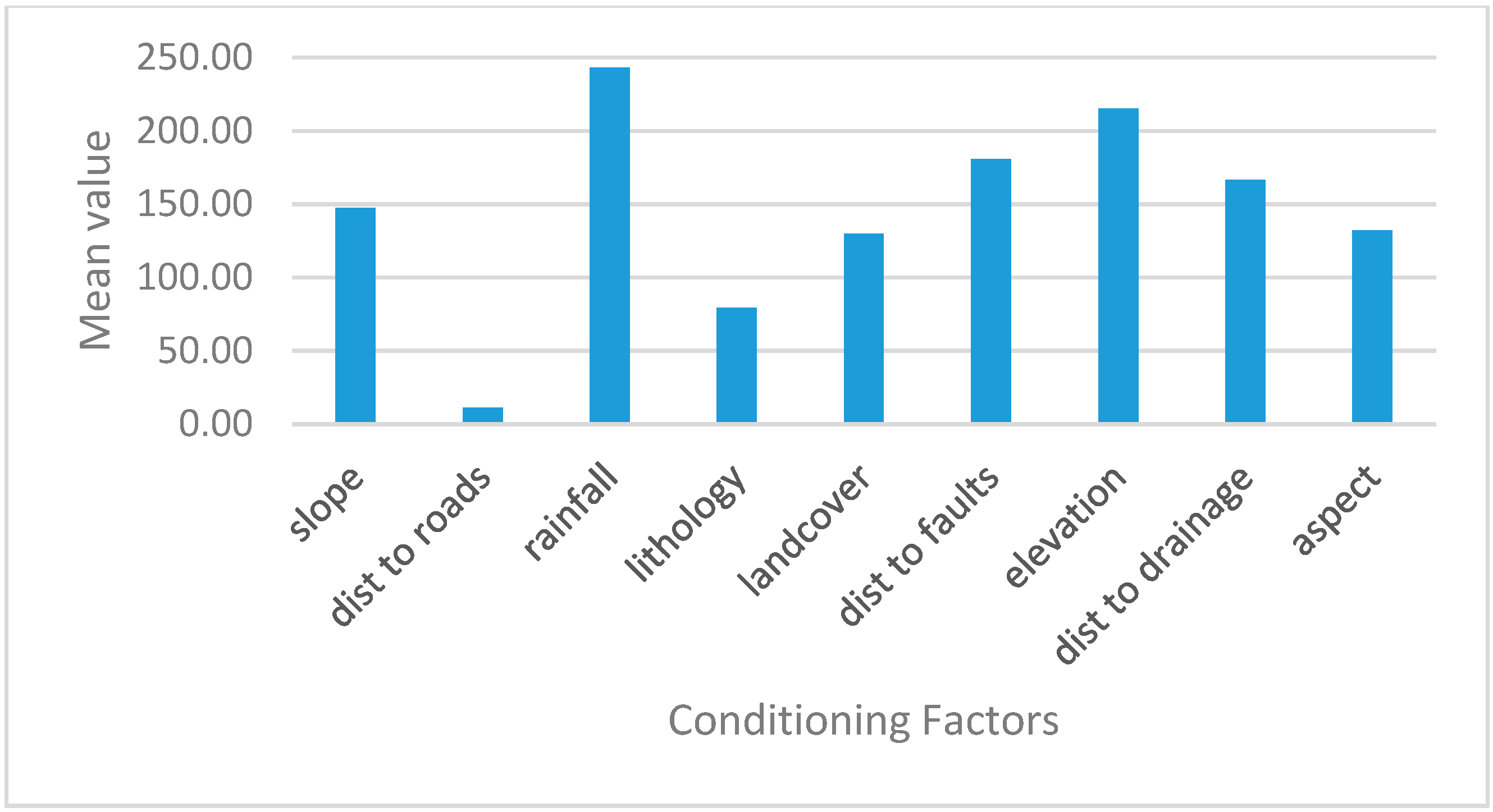
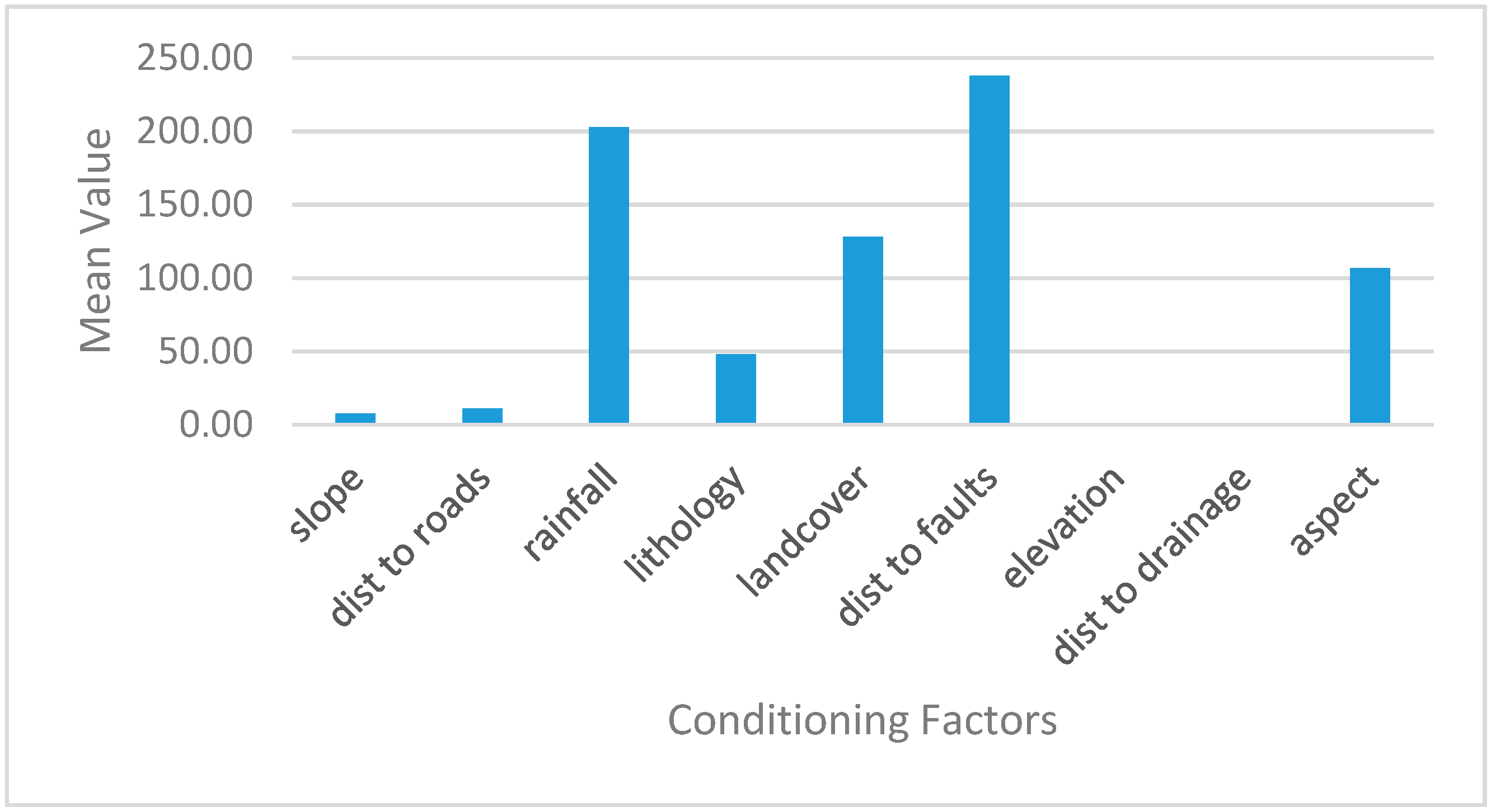
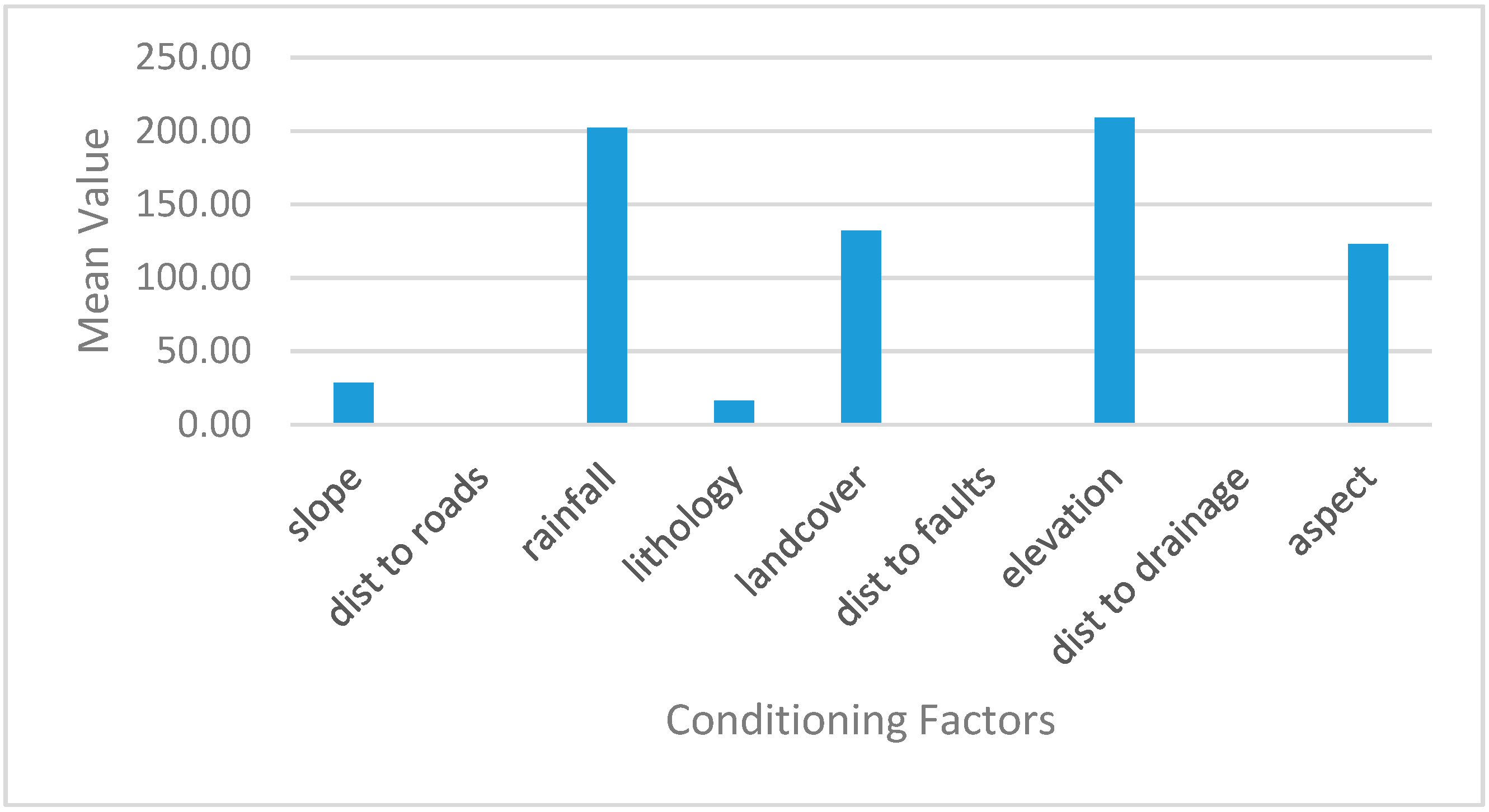
3.2. Landslide Conditioning Factors
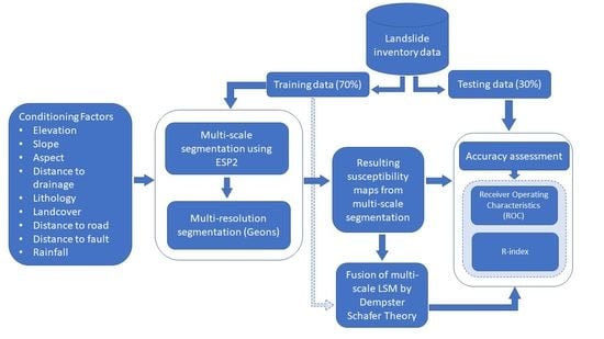
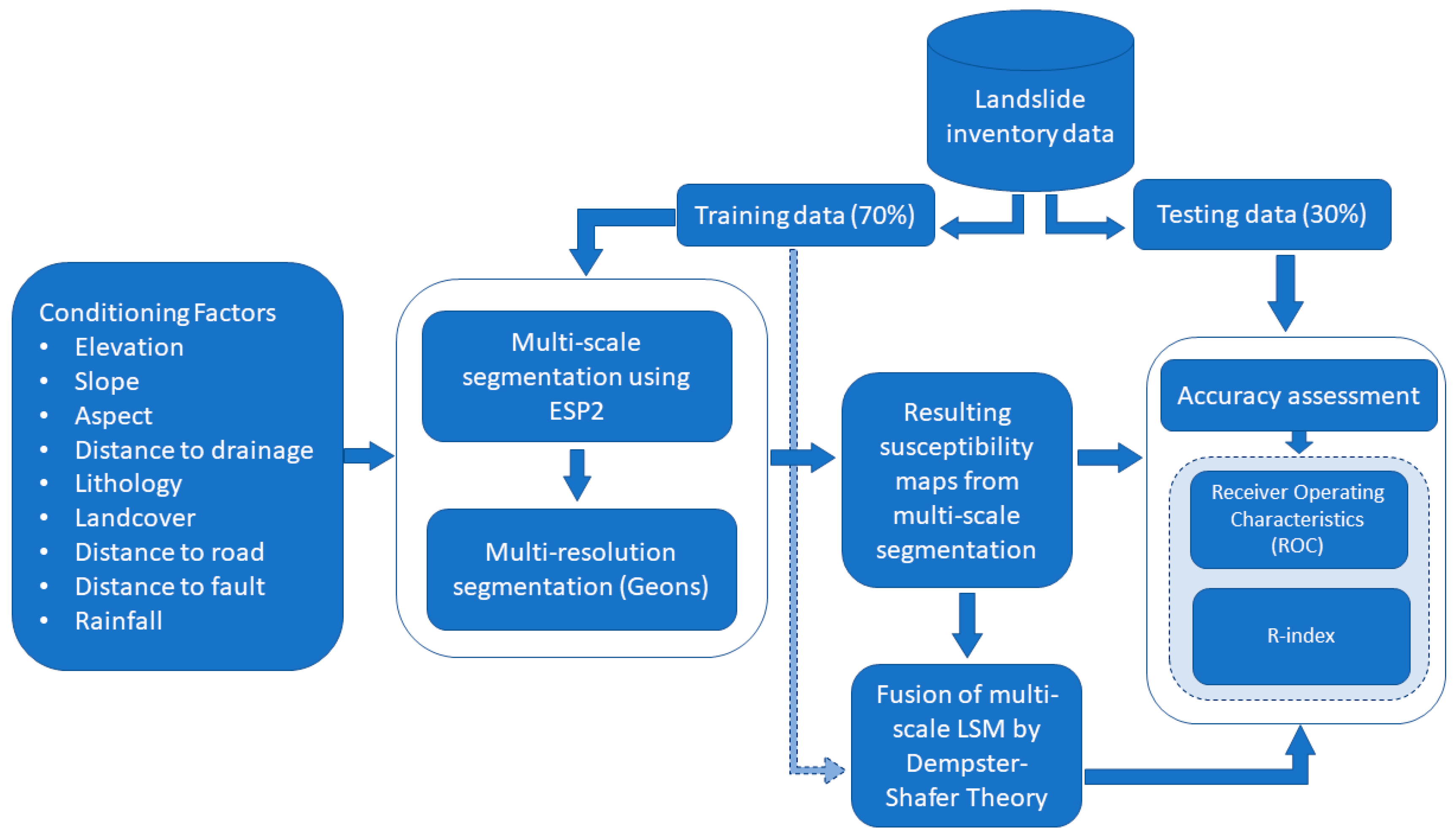
3.3. Methodology
3.3.1. Geons
3.3.2. Dempster–Shafer Theory (DST)
3.3.3. Fusion of Multiscale Results Via DST
4. Results
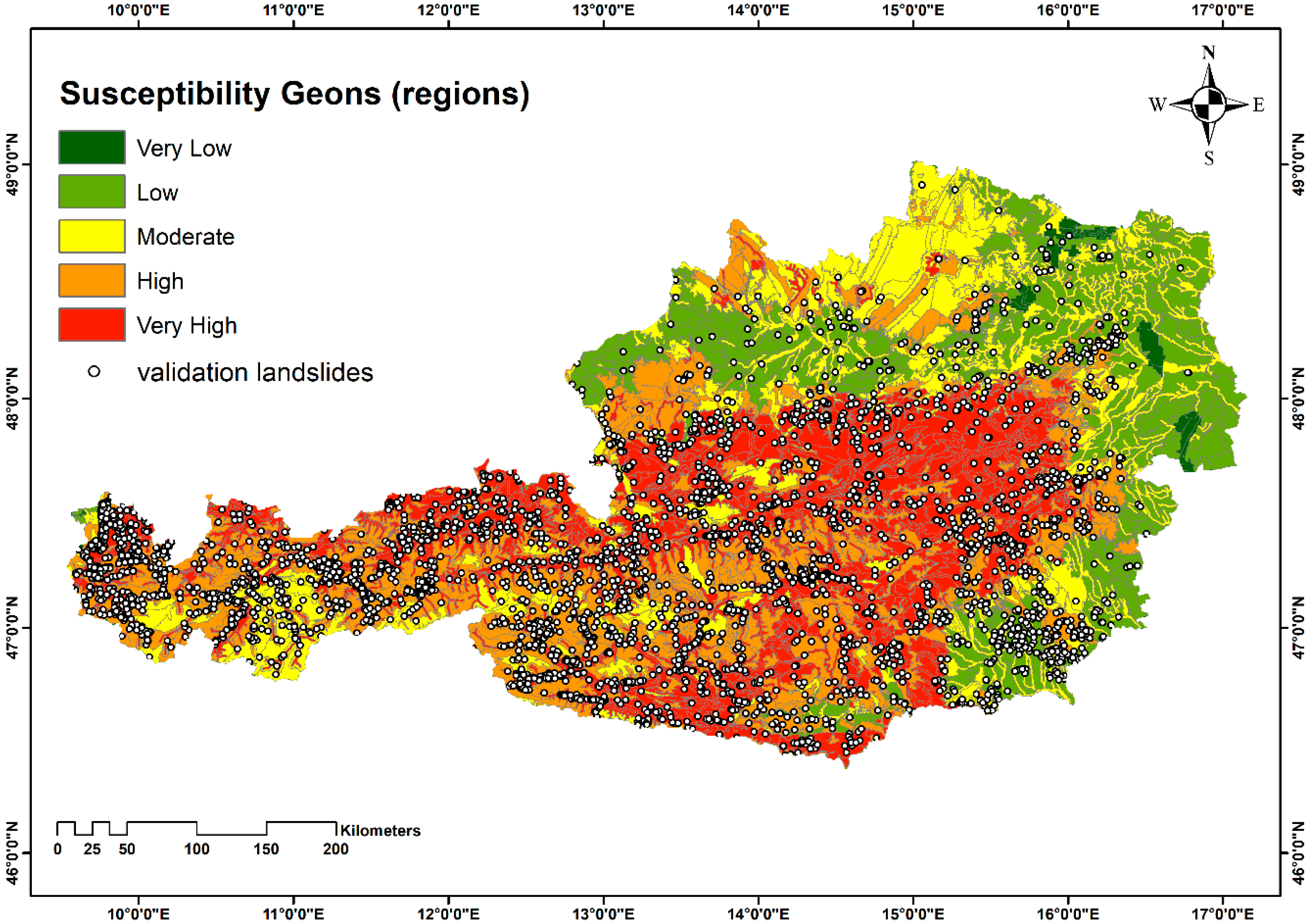
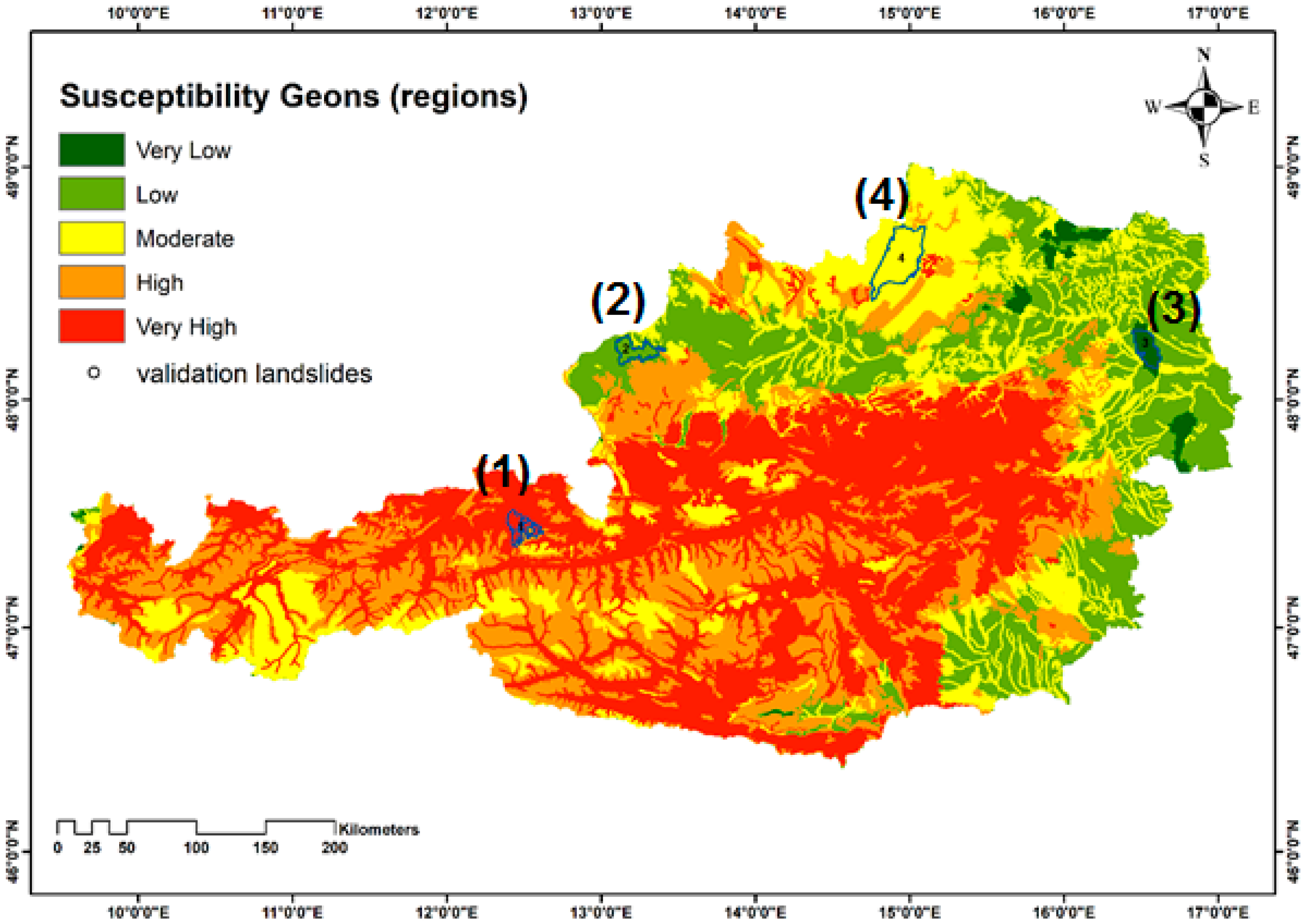
4.1. Geons
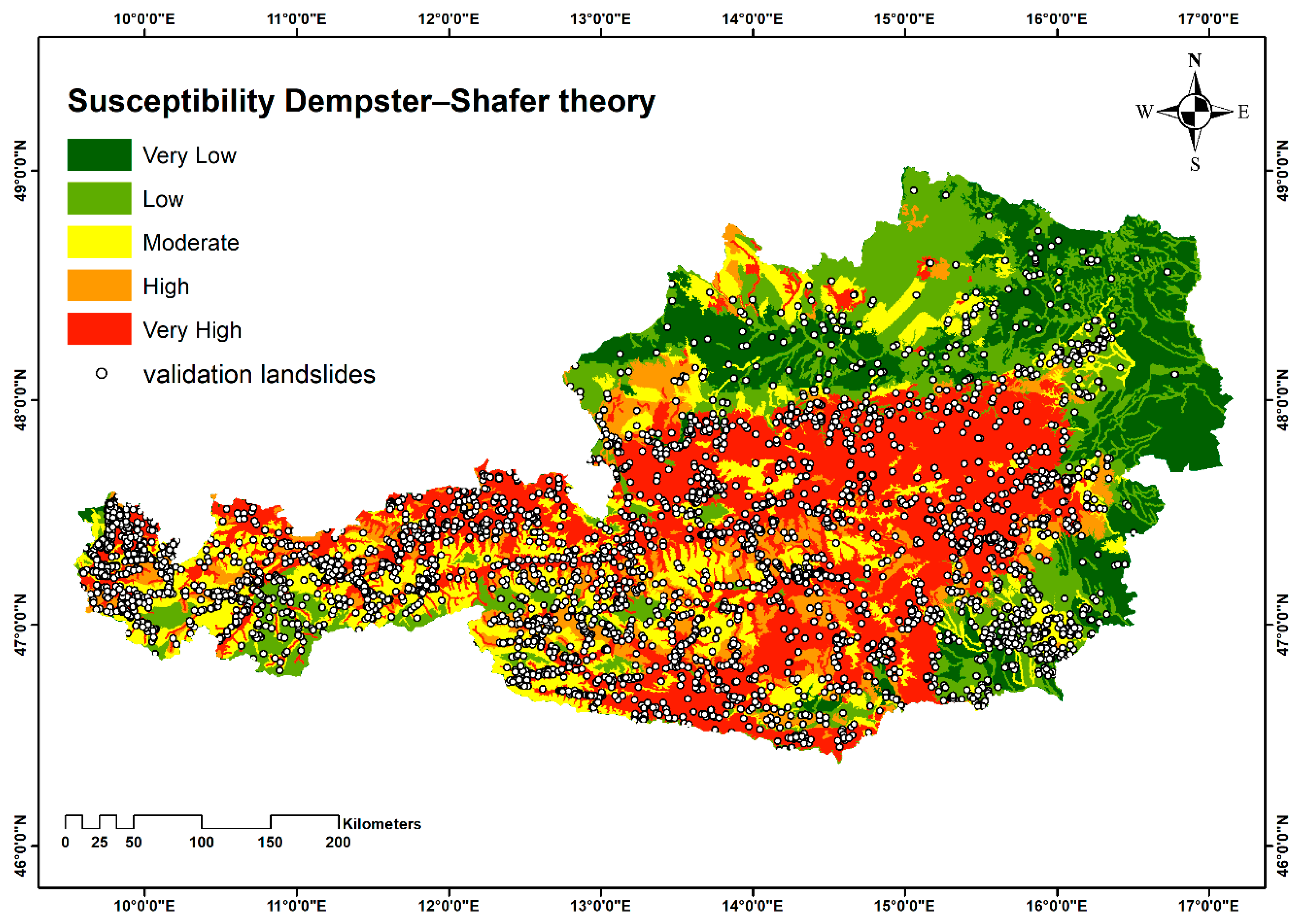
4.2. Dempster–Shafer
5. Validation
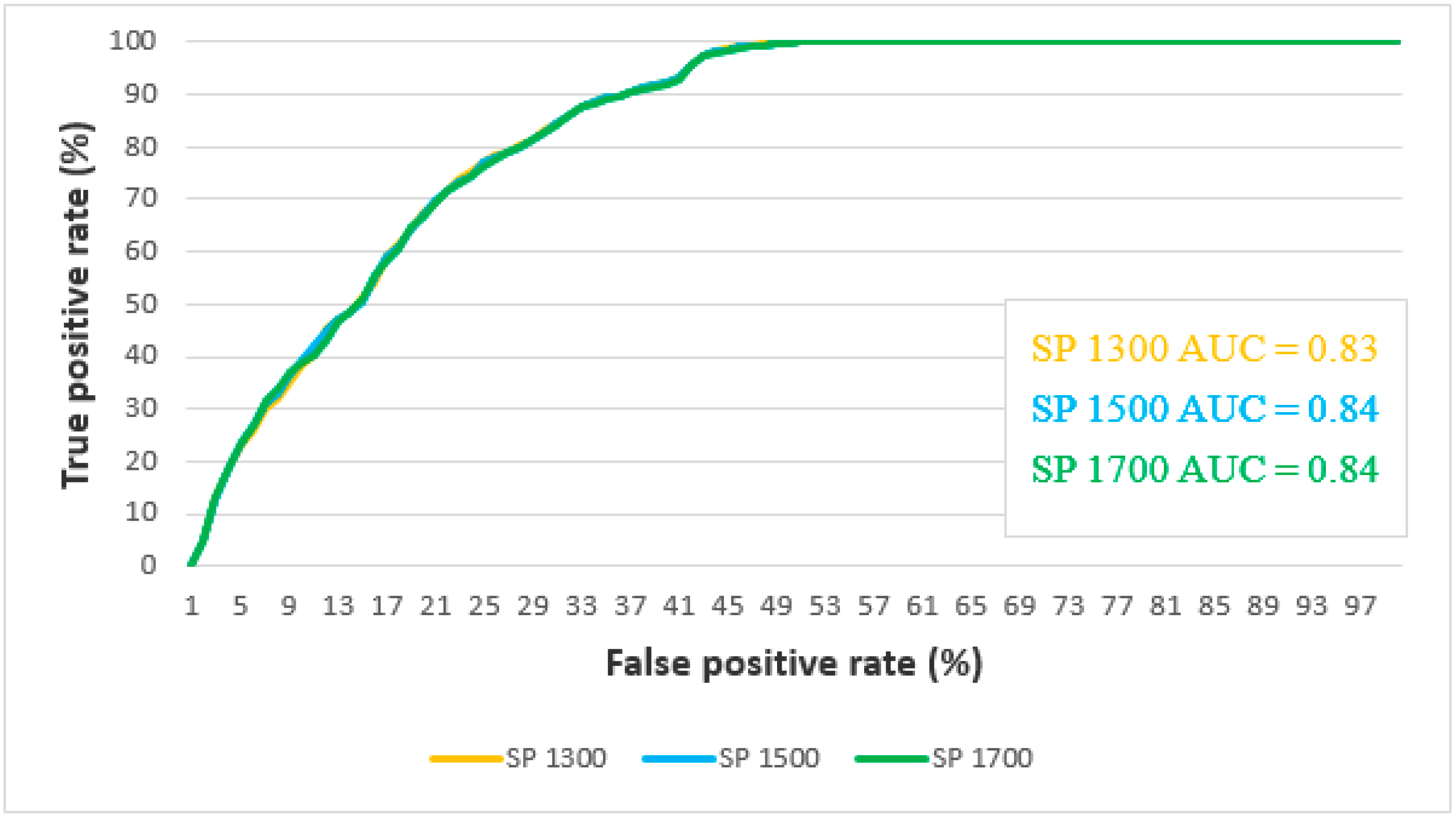
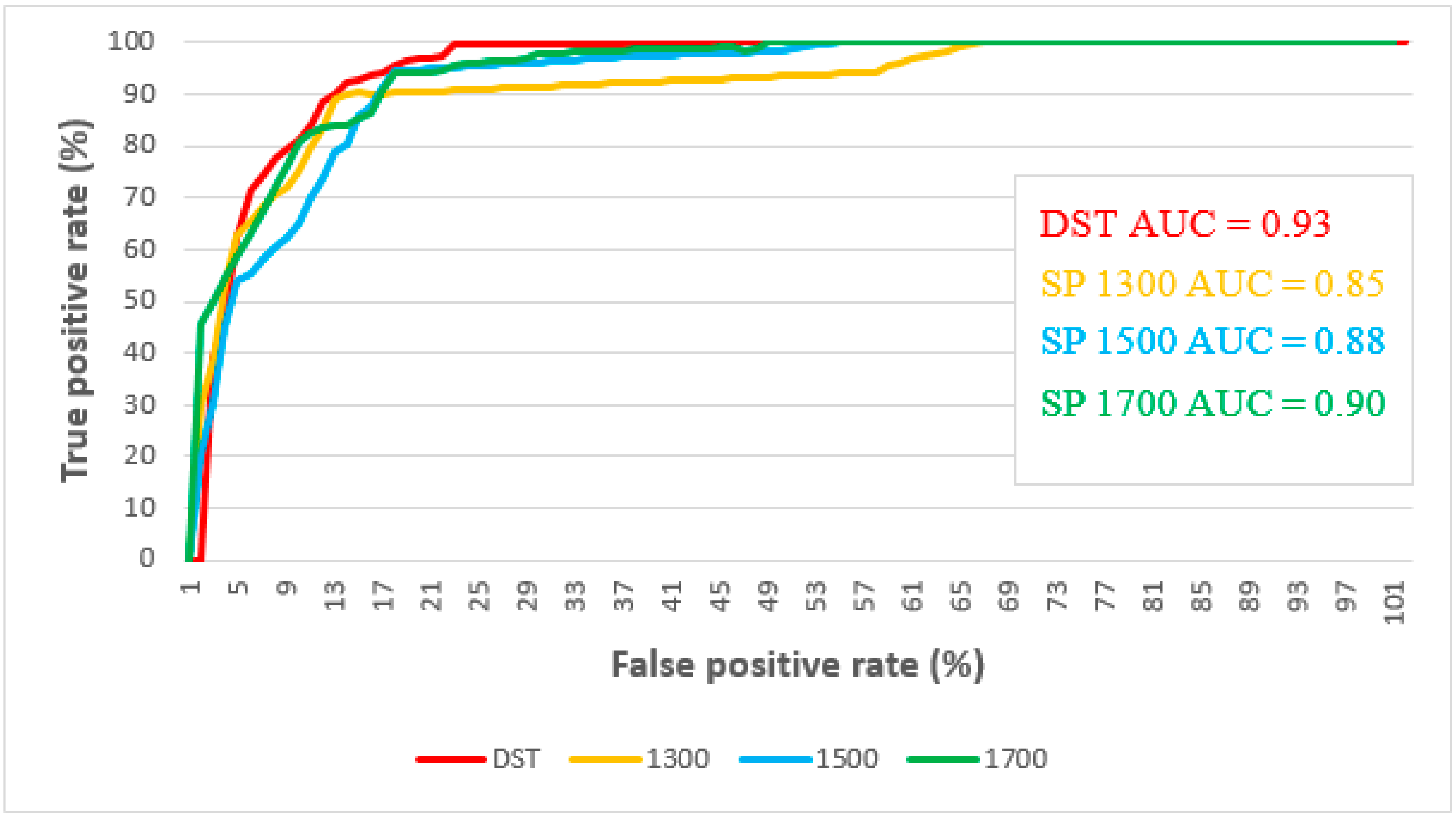
5.1. Receiver Operating Characteristics (ROC)
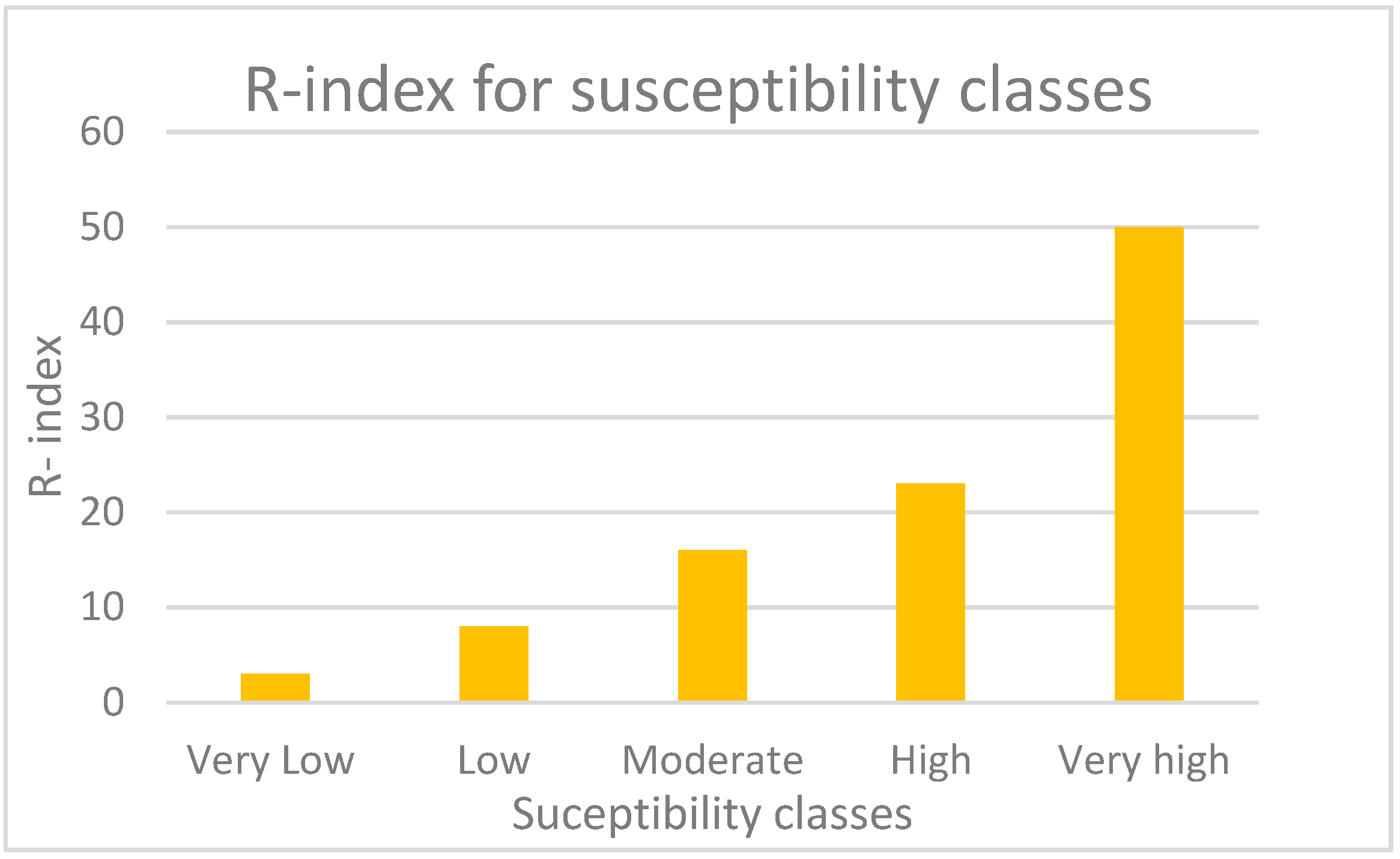
5.2. Relative Landslide Index (R-Index)
6. Discussion
7. Conclusions
Author Contributions
Funding
Acknowledgments
Conflicts of Interest
References
- Confuorto, P.; Di Martire, D.; Infante, D.; Novellino, A.; Papa, R.; Calcaterra, D.; Ramondini, M. Monitoring of remedial works performance on landslide-affected areas through ground-and satellite-based techniques. Catena 2019, 178, 77–89. [Google Scholar] [CrossRef]
- Pourghasemi, H.R.; Rahmati, O. Prediction of the landslide susceptibility: Which algorithm, which precision? Catena 2018, 162, 177–192. [Google Scholar] [CrossRef]
- Clerici, A.; Perego, S.; Tellini, C.; Vescovi, P. A procedure for landslide susceptibility zonation by the conditional analysis method. Geomorphology 2002, 48, 349–364. [Google Scholar] [CrossRef]
- Wilde, M.; Günther, A.; Reichenbach, P.; Malet, J.-P.; Hervás, J. Pan-European landslide susceptibility mapping: ELSUS Version 2. J. Maps 2018, 14, 97–104. [Google Scholar] [CrossRef]
- Lima, P.; Steger, S.; Glade, T.; Tilch, N.; Schwarz, L.; Kociu, A. Landslide Susceptibility Mapping at National Scale: A First Attempt for Austria. In Advancing Culture of Living with Landslides; Springer International Publishing: Ljubljana, Slovenia, 2017; pp. 943–951. [Google Scholar]
- Wu, Y.; Li, W.; Wang, Q.; Liu, Q.; Yang, D.; Xing, M.; Pei, Y.; Yan, S. Landslide susceptibility assessment using frequency ratio, statistical index and certainty factor models for the Gangu County, China. Arab. J. Geosci. 2016, 9, 84. [Google Scholar] [CrossRef]
- Haque, U.; Blum, P.; da Silva, P.F.; Andersen, P.; Pilz, J.; Chalov, S.R.; Malet, J.-P.; Auflič, M.J.; Andres, N.; Poyiadji, E.; et al. Fatal landslides in Europe. Landslides 2016, 13, 1545–1554. [Google Scholar] [CrossRef]
- Guzzetti, F.; Mondini, A.C.; Cardinali, M.; Fiorucci, F.; Santangelo, M.; Chang, K.-T. Chang. Landslide inventory maps: New tools for an old problem. Earth-Sci. Rev. 2012, 112, 42–66. [Google Scholar] [CrossRef]
- Hong, H.; Pradhan, B.; Xu, C.; Tien Bui, D. Spatial prediction of landslide hazard at the Yihuang area (China) using two-class kernel logistic regression, alternating decision tree and support vector machines. Catena 2015, 133, 266–281. [Google Scholar] [CrossRef]
- Tehrany, M.S.; Pradhan, B.; Jebur, M.N. Flood susceptibility analysis and its verification using a novel ensemble support vector machine and frequency ratio method. Stoch. Environ. Res. Risk Assess. 2015, 29, 1149–1165. [Google Scholar] [CrossRef]
- Roccati, A.; Faccini, F.; Luino, F.; Ciampalini, A.; Turconi, L. Heavy Rainfall Triggering Shallow Landslides: A Susceptibility Assessment by a GIS-Approach in a Ligurian Apennine Catchment (Italy). Water 2019, 11, 605. [Google Scholar] [CrossRef]
- Feizizadeh, B.; Jankowski, P.; Blaschke, T. A GIS based spatially-explicit sensitivity and uncertainty analysis approach for multi-criteria decision analysis. Comput. Geosci. 2014, 64, 81–95. [Google Scholar] [CrossRef] [PubMed]
- Roodposhti, M.S.; Aryal, J.; Pradhan, B. A Novel Rule-based Approach In Mapping Landslide Susceptibility. Sensors 2019, 19, 2274. [Google Scholar] [CrossRef] [PubMed]
- Pourghasemi, H.; Gayen, A.; Park, S.; Lee, C.-W.; Lee, S. Assessment of Landslide-Prone Areas and Their Zonation Using Logistic Regression, LogitBoost, and NaïveBayes Machine-Learning Algorithms. Sustainability 2018, 10, 3697. [Google Scholar] [CrossRef]
- Van Westen, C.J. Remote Sensing and GIS for Natural Hazards Assessment and Disaster Risk Management. In Treatise on Geomorphology; Academic Press: San Diego, CA, USA, 2013; pp. 259–298. [Google Scholar]
- Ghorbanzadeh, O.; Blaschke, T.; Aryal, J.; Gholaminia, K. A new GIS-based technique using an adaptive neuro-fuzzy inference system for land subsidence susceptibility mapping. J. Spat. Sci. 2018, 63, 1–17. [Google Scholar] [CrossRef]
- Kienberger, S.; Lang, S.; Zeil, P. Spatial vulnerability units—Expert-based spatial modelling of socio-economic vulnerability in the Salzach catchment, Austria. Nat. Hazards Earth Syst. Sci. 2009, 9, 767–778. [Google Scholar] [CrossRef]
- Khosravi, K.; Nohani, E.; Maroufinia, E.; Pourghasemi, H.R. A GIS-based flood susceptibility assessment and its mapping in Iran: A comparison between frequency ratio and weights-of-evidence bivariate statistical models with multi-criteria decision-making technique. Nat. Hazards 2016, 83, 947–987. [Google Scholar] [CrossRef]
- Rahmati, O.; Pourghasemi, H.R.; Zeinivand, H. Flood susceptibility mapping using frequency ratio and weights-of-evidence models in the Golastan Province, Iran. Geocarto Int. 2015, 31, 42–70. [Google Scholar] [CrossRef]
- Lee, S.; Pradhan, B. Landslide hazard mapping at Selangor, Malaysia using frequency ratio and logistic regression models. Landslides 2006, 4, 33–41. [Google Scholar] [CrossRef]
- Rahmati, O.; Zeinivand, H.; Besharat, M. Flood hazard zoning in Yasooj region, Iran, using GIS and multi-criteria decision analysis. Geomat. Nat. Hazards Risk 2015, 7, 1000–1017. [Google Scholar] [CrossRef]
- Ghorbanzadeh, O.; Feizizadeh, B.; Blaschke, T.; Khosravi, R. Spatially Explicit Sensitivity and Uncertainty Analysis for the landslide risk assessment of the Gas Pipeline Networks. In Proceedings of the 21st AGILE Conference on Geo-information Science, Lund, Sweden, 12–15 June 2018; pp. 1–7. [Google Scholar]
- Nampak, H.; Pradhan, B.; Manap, M.A. Application of GIS based data driven evidential belief function model to predict groundwater potential zonation. J. Hydrol. 2014, 513, 283–300. [Google Scholar] [CrossRef]
- Tehrany, M.S.; Pradhan, B.; Mansor, S.; Ahmad, N. Flood susceptibility assessment using GIS-based support vector machine model with different kernel types. Catena 2015, 125, 91–101. [Google Scholar] [CrossRef]
- Chapi, K.; Singh, V.P.; Shirzadi, A.; Shahabi, H.; Bui, D.T.; Pham, B.T.; Khosravi, K. A novel hybrid artificial intelligence approach for flood susceptibility assessment. Environ. Model. Softw. 2017, 95, 229–245. [Google Scholar] [CrossRef]
- Pradhan, B.; Lee, S.; Mansor, S.; Buchroithner, M.; Jamaluddin, N.; Khujaimah, Z. Utilization of optical remote sensing data and geographic information system tools for regional landslide hazard analysis by using binomial logistic regression model. J. Appl. Remote Sens. 2008, 2, 023542. [Google Scholar]
- Felicísimo, Á.M.; Cuartero, A.; Remondo, J.; Quirós, E. Mapping landslide susceptibility with logistic regression, multiple adaptive regression splines, classification and regression trees, and maximum entropy methods: A comparative study. Landslides 2013, 10, 175–189. [Google Scholar] [CrossRef]
- Hay, G.J.; Castilla, G. Geographic Object-Based Image Analysis (GEOBIA): A new name for a new discipline. In Object-Based Image Analysis; Springer: Berlin, Heidelberg, 2008; pp. 75–89. [Google Scholar]
- Benz, U.C.; Hofmann, P.; Willhauck, G.; Lingenfelder, I.; Heynen, M. Multi-resolution, object-oriented fuzzy analysis of remote sensing data for GIS-ready information. Isprs J. Photogramm. Remote Sens. 2004, 58, 239–258. [Google Scholar] [CrossRef]
- Blaschke, T.; Hay, G.J.; Kelly, M.; Lang, S.; Hofmann, P.; Addink, E.; Feitosa, R.Q.; Van der Meer, F.; Van der Werff, H.; Van Coillie, F. Geographic object-based image analysis–towards a new paradigm. Isprs J. Photogramm. Remote Sens. 2014, 87, 180–191. [Google Scholar] [CrossRef]
- Lang, S.; Kienberger, S.; Tiede, D.; Hagenlocher, M.; Pernkopf, L. Geons—Domain-specific regionalization of space. Cartogr. Geogr. Inf. Sci. 2014, 41, 214–226. [Google Scholar] [CrossRef]
- Costa, H.; Foody, G.M.; Boyd, D.S. Supervised methods of image segmentation accuracy assessment in land cover mapping. Remote Sens. Environ. 2018, 205, 338–351. [Google Scholar] [CrossRef]
- Drăguţ, L.; Csillik, O.; Eisank, C.; Tiede, D. Automated parameterisation for multi-scale image segmentation on multiple layers. Isprs J. Photogramm. Remote Sens. 2014, 88, 119–127. [Google Scholar] [CrossRef]
- Shahabi, H.; Jarihani, B.; Tavakkoli Piralilou, S.; Chittleborough, D.; Avand, M.; Ghorbanzadeh, O. A Semi-Automated Object-Based Gully Networks Detection Using Different Machine Learning Models: A Case Study of Bowen Catchment, Queensland, Australia. Sensors 2019, 19, 4893. [Google Scholar] [CrossRef]
- Ghorbanzadeh, O.; Blaschke, T.; Gholamnia, K.; Meena, S.R.; Tiede, D.; Aryal, J. Evaluation of Different Machine Learning Methods and Deep-Learning Convolutional Neural Networks for Landslide Detection. Remote Sens. 2019, 11, 196. [Google Scholar] [CrossRef]
- Blaschke, T.; Piralilou, S.T. The near-decomposability paradigm re-interpreted for place-based GIS. In Proceedings of the 1st Workshop on Platial Analysis (PLATIAL’18), Heidelberg, Germany, 20–21 September 2018. [Google Scholar]
- Yager, R.R.; Liu, L. Classic Works of the Dempster-Shafer Theory of Belief Functions; Springer: Berlin, Heidelberg, 2008; Volume 219. [Google Scholar]
- Mezaal, M.; Pradhan, B.; Rizeei, H. Improving Landslide Detection from Airborne Laser Scanning Data Using Optimized Dempster–Shafer. Remote Sens. 2018, 10, 1029. [Google Scholar] [CrossRef]
- Pham, B.T.; Bui, D.T.; Prakash, I.; Dholakia, M. Hybrid integration of Multilayer Perceptron Neural Networks and machine learning ensembles for landslide susceptibility assessment at Himalayan area (India) using GIS. Catena 2017, 149, 52–63. [Google Scholar] [CrossRef]
- Tavakkoli Piralilou, S.; Shahabi, H.; Jarihani, B.; Ghorbanzadeh, O.; Blaschke, T.; Gholamnia, K.; Meena, S.R.; Aryal, J. Landslide Detection Using Multi-Scale Image Segmentation and Different Machine Learning Models in the Higher Himalayas. Remote Sens. 2019, 11, 2575. [Google Scholar] [CrossRef]
- Petschko, H.; Brenning, A.; Bell, R.; Goetz, J.; Glade, T. Assessing the quality of landslide susceptibility maps–case study Lower Austria. Nat. Hazards Earth Syst. Sci. 2014, 14, 95–118. [Google Scholar] [CrossRef]
- Tsangaratos, P.; Ilia, I. Comparison of a logistic regression and Naïve Bayes classifier in landslide susceptibility assessments: The influence of models complexity and training dataset size. Catena 2016, 145, 164–179. [Google Scholar] [CrossRef]
- Ayalew, L.; Yamagishi, H. The application of GIS-based logistic regression for landslide susceptibility mapping in the Kakuda-Yahiko Mountains, Central Japan. Geomorphology 2005, 65, 15–31. [Google Scholar] [CrossRef]
- Meena, S.R.; Ghorbanzadeh, O.; Blaschke, T. A Comparative Study of Statistics-Based Landslide Susceptibility Models: A Case Study of the Region Affected by the Gorkha Earthquake in Nepal. Isprs Int. J. Geo-Inf. 2019, 8, 94. [Google Scholar] [CrossRef]
- Yalcin, A.; Bulut, F. Landslide susceptibility mapping using GIS and digital photogrammetric techniques: A case study from Ardesen (NE-Turkey). Nat. Hazards 2006, 41, 201–226. [Google Scholar] [CrossRef]
- Bartelletti, C.; Giannecchini, R.; D’Amato Avanzi, G.; Galanti, Y.; Mazzali, A. The influence of geological–morphological and land use settings on shallow landslides in the Pogliaschina T. basin (northern Apennines, Italy). J. Maps 2017, 13, 142–152. [Google Scholar] [CrossRef]
- Persichillo, M.G.; Bordoni, M.; Meisina, C. The role of land use changes in the distribution of shallow landslides. Sci. Total Environ. 2017, 574, 924–937. [Google Scholar] [CrossRef] [PubMed]
- Cordeira, J.M.; Stock, J.; Dettinger, M.D.; Young, A.M.; Kalansky, J.F.; Ralph, F.M. A 142-year Climatology of Northern California Landslides and Atmospheric Rivers. Bull. Am. Meteorol. Soc. 2019, 100, 1499–1509. [Google Scholar] [CrossRef]
- Dang, V.-H.; Dieu, T.B.; Tran, X.-L.; Hoang, N.-D. Hoang. Enhancing the accuracy of rainfall-induced landslide prediction along mountain roads with a GIS-based random forest classifier. Bull. Eng. Geol. Environ. 2018, 78, 2835–2849. [Google Scholar] [CrossRef]
- Chen, W.; Pourghasemi, H.R.; Naghibi, S.A. A comparative study of landslide susceptibility maps produced using support vector machine with different kernel functions and entropy data mining models in China. Bull. Eng. Geol. Environ. 2017, 77, 647–664. [Google Scholar] [CrossRef]
- Walter, V.; Fritsch, D. Automatic verification of GIS data using high resolution multispectral data. Int. Arch. Photogramm. Remote Sens. 1998, 32, 485–490. [Google Scholar]
- Blaschke, T. Object based image analysis for remote sensing. Isprs J. Photogramm. Remote Sens. 2010, 65, 2–16. [Google Scholar] [CrossRef]
- Hagenlocher, M.; Kienberger, S.; Lang, S.; Blaschke, T. Implications of spatial scales and reporting units for the spatial modelling of vulnerability to vector-borne diseases. Gi_Forum 2014, 2014, 197. [Google Scholar]
- Tiede, D.; Lang, S.; Albrecht, F.; Holbling, D. Object-based Class Modeling for Cadastre-constrained Delineation of Geo-objects. Photogramm. Eng. Remote Sens. 2010, 76, 193–202. [Google Scholar] [CrossRef]
- Drǎguţ, L.; Tiede, D.; Levick, S.R. ESP: A tool to estimate scale parameter for multiresolution image segmentation of remotely sensed data. Int. J. Geogr. Inf. Sci. 2010, 24, 859–871. [Google Scholar] [CrossRef]
- Foley, B.G. A Dempster-Shafer Method for Multi-Sensor Fusion. 2012. [Google Scholar]
- Feizizadeh, B.; Blaschke, T.; Nazmfar, H. GIS-based ordered weighted averaging and Dempster–Shafer methods for landslide susceptibility mapping in the Urmia Lake Basin, Iran. Int. J. Digit. Earth 2014, 7, 688–708. [Google Scholar] [CrossRef]
- Martin, R.; Zhang, J.; Liu, C. Dempster–Shafer theory and statistical inference with weak beliefs. Stat. Sci. 2010, 25, 72–87. [Google Scholar] [CrossRef]
- Eastman, J. IDRISI Selva: Guide to GIS and Image Processing; Clark Labratories, Clark University: Worcester, MA, USA, 2012. [Google Scholar]
- Feizizadeh, B. A Novel Approach of Fuzzy Dempster–Shafer Theory for Spatial Uncertainty Analysis and Accuracy Assessment of Object-Based Image Classification. IEEE Geosci. Remote Sens. Lett. 2018, 15, 18–22. [Google Scholar] [CrossRef]
- Baraldi, P.; Zio, E. A comparison between probabilistic and dempster-shafer theory approaches to model uncertainty analysis in the performance assessment of radioactive waste repositories. Risk Anal. Int. J. 2010, 30, 1139–1156. [Google Scholar] [CrossRef][Green Version]
- Rottensteiner, F.; Trinder, J.; Clode, S.; Kubik, K. Using the Dempster–Shafer method for the fusion of LIDAR data and multi-spectral images for building detection. Inf. Fusion 2005, 6, 283–300. [Google Scholar] [CrossRef]
- Ghorbanzadeh, O.; Valizadeh Kamran, K.; Blaschke, T.; Aryal, J.; Naboureh, A.; Einali, J.; Bian, J. Spatial Prediction of Wildfire Susceptibility Using Field Survey GPS Data and Machine Learning Approaches. Fire 2019, 2, 43. [Google Scholar] [CrossRef]
- Ghorbanzadeh, O.; Rostamzadeh, H.; Blaschke, T.; Gholaminia, K.; Aryal, J. A new GIS-based data mining technique using an adaptive neuro-fuzzy inference system (ANFIS) and k-fold cross-validation approach for land subsidence susceptibility mapping. Nat. Hazards 2018, 94, 497–517. [Google Scholar] [CrossRef]
- Ghorbanzadeh, O.; Feizizadeh, B.; Blaschke, T. Multi-criteria risk evaluation by integrating an analytical network process approach into GIS-based sensitivity and uncertainty analyses. Geomat. Nat. Hazards Risk 2018, 9, 127–151. [Google Scholar] [CrossRef]


| Validation Methods | Sensitivity Class | Number of Pixels | Area (m2) | Area Percent (ni) | Number of Landslides | Landslide Percent (Ni) | R-Index |
|---|---|---|---|---|---|---|---|
| GEONS | Very Low | 558,779 | 2,011,604,400 | 2.35 | 5 | 0.26 | 3 |
| Low | 4,763,839 | 17,149,820,400 | 20.00 | 110 | 5.81 | 8 | |
| Moderate | 3,650,614 | 13,142,210,400 | 15.32 | 162 | 8.56 | 16 | |
| High | 6,577,120 | 23,677,632,000 | 27.61 | 424 | 22.41 | 23 | |
| Very high | 8,272,806 | 29,782,101,600 | 34.73 | 1191 | 62.95 | 50 |
© 2019 by the authors. Licensee MDPI, Basel, Switzerland. This article is an open access article distributed under the terms and conditions of the Creative Commons Attribution (CC BY) license (http://creativecommons.org/licenses/by/4.0/).
Share and Cite
Gudiyangada Nachappa, T.; Tavakkoli Piralilou, S.; Ghorbanzadeh, O.; Shahabi, H.; Blaschke, T. Landslide Susceptibility Mapping for Austria Using Geons and Optimization with the Dempster-Shafer Theory. Appl. Sci. 2019, 9, 5393. https://doi.org/10.3390/app9245393
Gudiyangada Nachappa T, Tavakkoli Piralilou S, Ghorbanzadeh O, Shahabi H, Blaschke T. Landslide Susceptibility Mapping for Austria Using Geons and Optimization with the Dempster-Shafer Theory. Applied Sciences. 2019; 9(24):5393. https://doi.org/10.3390/app9245393
Chicago/Turabian StyleGudiyangada Nachappa, Thimmaiah, Sepideh Tavakkoli Piralilou, Omid Ghorbanzadeh, Hejar Shahabi, and Thomas Blaschke. 2019. "Landslide Susceptibility Mapping for Austria Using Geons and Optimization with the Dempster-Shafer Theory" Applied Sciences 9, no. 24: 5393. https://doi.org/10.3390/app9245393
APA StyleGudiyangada Nachappa, T., Tavakkoli Piralilou, S., Ghorbanzadeh, O., Shahabi, H., & Blaschke, T. (2019). Landslide Susceptibility Mapping for Austria Using Geons and Optimization with the Dempster-Shafer Theory. Applied Sciences, 9(24), 5393. https://doi.org/10.3390/app9245393