Using Acoustic Emission Measurements for Ice-Melting Detection

Featured Application

This work contributes to the development of a monitoring system for the remote detection, localization and quantification of melting ice. Acoustic emission measurements enable the remote monitoring in an environment where the region of interest is neither optically nor physically accessible. The kerosene tank of civil aircraft is one example where the aforementioned accessibility is only achieved with high costs and extensive labor. This is why inter alia aircraft operators that perform the daily maintenance of civil aircraft are interested in such an inspection method. Here the detection of ice inside the fuel tanks increases the operational efficiency as well as the safety for the ground personnel.

Abstract

Aircraft operators being faced with water accumulation in fuel tanks on a daily basis and are looking for reliable detection systems to determine the remaining amount of accumulated ice during maintenance after flight. Using such a technology, an increase in the safety and efficiency of the aircraft operation would be possible in this highly competitive market. This article presents the use of the Acoustic Emission Technique (AE) for the reliable and non-invasive monitoring of the melting of ice in fuel tanks. This technology is in principle based on the fact that a phase transition comes frequently along with stress relaxation that can be used for monitoring the process. Therefore, the melting of water can, in essence, be monitored with AE without accessing the ice directly. The analysis of the AE signals has been carried out in the time domain since it was the melting of ice needed to be monitored as a function of temperature rise time. The insights presented in this paper can possibly lead to new technologies for ice detection, especially in remote areas that are not easily accessible with other techniques.

1. Introduction

Since the beginning of aviation, innovation in technologies and operational procedures have steadily increased comfort, performance and safety of air transport. Especially the latter aspect leads to a continuously decreasing number of fatal accidents even though the number of passengers is steadily increasing. In this context, it is important that also aging aircraft types are retrofit equipped with modern technologies whenever feasible.

Besides new technological developments, the competition on the European as well as the global aviation market increases continuously. This pushes aircraft operators towards more efficient processes. In order to enhance efficiency, many key innovations focus on the reduction of scheduled and unscheduled grounding time (downtime) of the aircraft which is the time an aircraft is not available for flying. However, the procedure to remove liquid water from the fuel systems, called the draining procedure, requires time for the frozen water inside the tank to melt. The draining procedure makes use of the fact that liquid water, as well as ice, have a higher density than kerosene. Therefore, liquid water can be removed from the fuel tank by opening so-called drain valves at the lowest point of the tank and let the water run out of the tank. As this only removes liquid water from the tank, one must wait until all frozen water is molten. The time needed for the ice to melt depends on the inner temperature of the tank and on the outer surrounding temperature. Especially at cold winter times, scheduled downtimes are insufficient to melt all frozen water. A detailed description of the draining procedure and the problem occurring during the daily aircraft operation can be found in Stamm et al. [1].

The real-time detection of remaining ice inside the fuel tank will thus contribute to the optimization of the draining procedure that is performed to remove liquid water from the fuel tank enabling in this way a considerable reduction of costly downtimes. For the operation in the hangar by aircraft technicians, a mobile, small and easy-to-use AE system that can monitor the melting ice from outside the tank is required. To match these requirements already in laboratory experiments, a low-priced system with off-the-shelf components is used to perform presented experiments.

1.1. Water in Fuel Tanks

During the daily operation of aircraft, water accumulates inside the aircraft fuel tanks and freezes if the outside air reaches sub-zero temperatures. Different possibilities and root causes of water contamination in jet fuel are discussed in Baena-Zambrana et al. [2]. Besides the contaminated fuel that is used to fill up the aircraft tanks, water vapor condensation inside the aircraft fuel tank also leads to water accumulation inside the tank. Liquid water finally disturbs fuel quantity meters and enables microbiological corrosion whereas frozen water can harm the internal systems and structures by e.g., blocking valves or bursting pipes by freezing inside the pipes.

1.2. AE Monitoring of Melting Ice

AE is a well-established monitoring technique in the field of non-destructive testing (NDT) and many reviews mention applications in the fields of condition and process monitoring and defect detection. Li [3] gives a suitable review of using AE for monitoring metal cutting processes and discusses related signal processing methodologies including time series analysis, FFT, wavelet transform, etc.. Examples for AE-based condition monitoring and defect detection in the civil sector are described in Behnia et al. [4], Zaki et al. [5] as well as Vestrynge et al. [6] who present their work on monitoring concrete structures. Schiavi et al. [7] present their work which shows that AE can also applied to monitor the brittle materials during compression tests.

Additionally, Boyd and Varley [8] list several chemical processes that were monitored with AE such as the addition of sodium carbonate to calcium chloride [9], metal-acid reaction [10] or the solid-phase transitions of ${\mathrm{C}}_2{\mathrm{Cl}}_6$ [11].

Sawada et al. [12] measured the acoustic signals during the freezing and melting of super cooled distilled water. Melting and freezing are accompanied by acoustic activity that is more intense during the melting. This is the general behavior of phase transitions with a volume decrease being acoustically more active than transitions with volume expansion [12]. Wentzell et al. [13] also measured the initial melting phase of distilled water. Since this is believed to be predominated by crystal fracture due to the high temperature gradient between the sample and the surrounding temperature, no or only a negligible number of events that occur due to the phase transition itself are measured. Finally, the mentioned literature provides only the time histogram of acoustic events during the melting of ice and no additional analysis of the acquired data.

Unlike melting processes, AE measurements on crystallization processes are discussed in some publications, e.g., by Lube and Zlatkin [14] and Ersen et al. [15] who use AE to estimate the crystal purity during the growing of ruby and leuco-sapphire crystal and effect of malic and citric acid on the crystallization of gypsum respectively. Furthermore, Wang and Huang [16] performed AE measurement on crystallization processes of salicylic acid and concluded that AE can be used as a reliable technique to monitor the development of the crystallization process.

The possibility of using the AE technique to monitor the melting of ice, first using tab water, is further explored and documented in this paper. The experimental setup that allows a controlled environmental conditions will be explained in the following.

2. Experimental Setup

For the AE measurement during melting and freezing, an experimental setup was built that allows the controlled freezing and melting of a sample while keeping the environmental noise at a minimal level. In the following, the AE measurement setup that meets the industry requirements described above and the thermostatic setup are explained.

2.1. Data Acquisition and Processing

A good review of AE measurements of chemical processes is given in Grosse and Ohtsu [17] where the general approach, usage and advantages of acoustic emission measurements are discussed. In addition, a general AE setup is described which usually contains an acoustic sensor, followed by a filtering and amplification of the signals and dedicated signal analysis by the CPU. In the following all three parts will be explained separately.

The most common AE sensors are piezoelectric (PZT) sensors that use the piezoelectric effect which transforms elastic motions into voltages [17]. In this work, the commercial broadband piezoelectric sensor “VS30-V” from the Vallen Systeme GmbH with a flat frequency response between 25 to 80 $\mathrm{kHz}$ [18].

The PZT sensor is connected to an AC coupled preamplifier “Model 5670” by Olympus NDT Inc. This broadband preamplifier provides a very-low-noise 40 $\mathrm{dB}$ amplification of ultrasonic signals with a flat ($\pm 1.5$ $\mathrm{dB}$) response in a frequency range of 50 $\mathrm{kHz}$–10 $\mathrm{MHz}$ [19]. The advantage of the bandwidth that does not match with the full operating frequency of the PZT is that frequencies below 50 $\mathrm{kHz}$ are not amplified which reduces the picked up ambient noise. Thereafter, a “PicoScope 2205A” USB oscilloscope digitizes and saves the waveforms with a sampling frequency of $f_s=1.565$ $\mathrm{MHz}$. The oscilloscope operates in a simple edge threshold trigger mode with a trigger level of ${\mathrm{V}}_{\mathrm{THD}}=+10$ $\mathrm{mV}$ which was approximately two time the environmental noise at the beginning of the experiments. With every trigger, a time windows with a length of t = 2 $\mathrm{ms}$ (trigger point at $t_{trigger}$ = $20\%$ = $0.4$ $\mathrm{ms}$) is saved in a file that contains the time of occurrence.

The settings of the oscilloscope define some additional parameters that are commonly used in AE:

• hit definition time (HDT)
• hit lockout time (HLT)
• peak definition time (PDT)

Classical AE systems allow the explicit setting of these parameters for a optimized operation in certain conditions. With the setup used in this study, these parameters are given by the operating mode of the oscilloscope and no additional (software implemented) realization of these parameters is implemented. The PDT = $1.6$ $\mathrm{ms}$ is given by the recorded time window for each AE event. The HDT and HLT are not explicitly set but implicitly given by the oscilloscope settings. The recorded time window and the duration of the AE previous event determine the HDT such as $\mathrm{D}+\mathrm{HDT}=1.6$ $\mathrm{ms}$. Due to the short duration of the expected AE events ($\overline{\mathrm{D}}\approx$ 15% of the recording time window) and the low quantity of signals, no HLT is required and it can be assumed as zero.

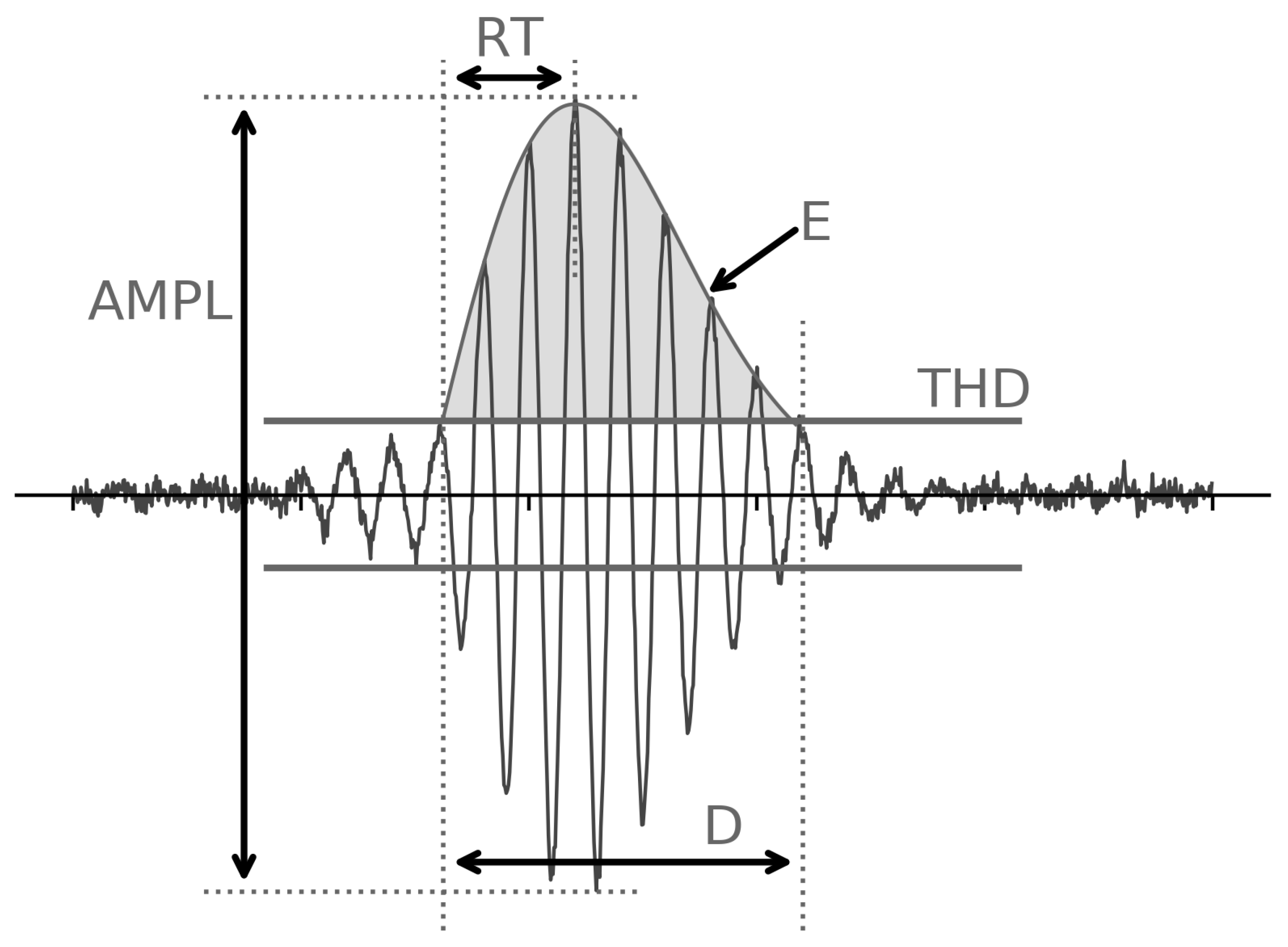
The post-processing of the recorded transients is done in real time in an additional module of the data acquisition software, which is coded in Python 3.7. Figure 1 shows a typical acoustic burst and some parameters that are also listed in Grosse and Ohtsu [17] and typically used for parameter-based analysis. The following parameters are calculated for each transient:

• Amplitude (AMPL) in [$\mathrm{mV}$]
• Duration (D) in [$\mathrm{ms}$]
• Rise time (RT) in [$\mathrm{ms}$]
• Energy (E) in [$\mathrm{ms}$ × $\mathrm{mV}$]

2.2. Temperature Controlling System

To measure the acoustic activity of melting ice, not only an AE measurement system but also a stable thermostatic setup is essential and this was achieved by an in-house-built device that monitors and controls the temperature in a closed volume. To reach a stable temperature in the range of $-15$ to $+45$ ${}^{\circ }\mathrm{C}$, two Peltier cooler modules (Adaptive APH-199-14-15-E) are driven by a controller of Meerstetter Engineering GmbH controller (Meerstetter TEC-1090-HV) and the accompanying software (TEC Service V 3.00).

A 10 $\mathrm{k}$$\mathsf{\Omega }$ NTC temperature sensor measures the air temperature inside the box and provides the feedback for the software to adjust the cooling power of the Peltier elements. To guarantee an equally distributed temperature inside the box with an inner volume of ca. $4\times 4\times 10{\mathrm{cm}}^3$, a ventilator is constantly circulating the air.

The explained setup provides, depending on the experiment, a constant temperature or a linear temperature change until reaching a target temperature. This exactly enables the freezing and melting of a water under controlled environmental conditions.

2.3. Sensor Setting

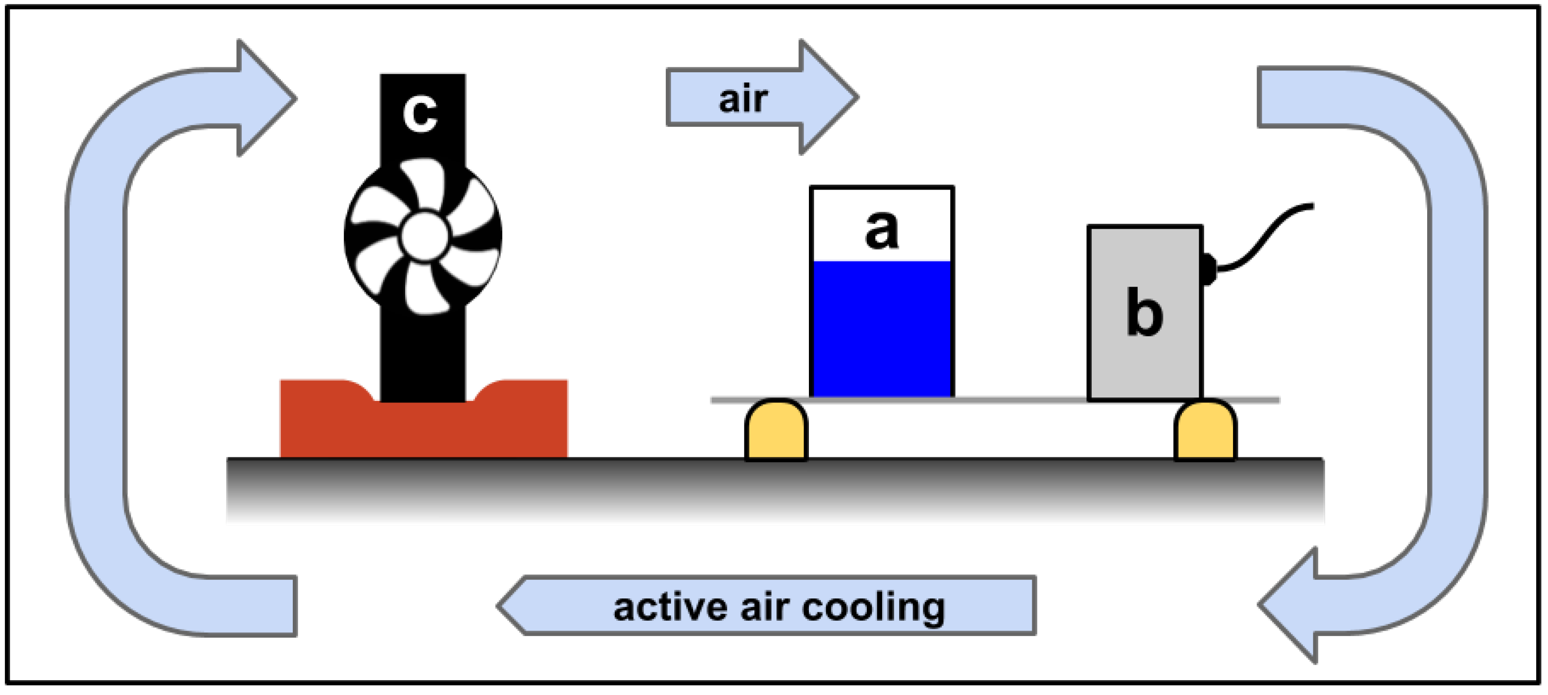
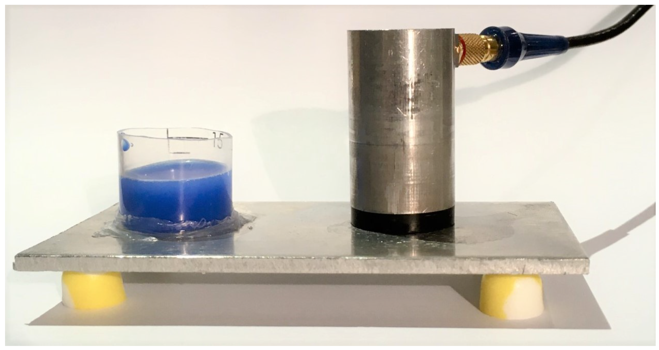
Figure 2 and Figure 3 show a sketch and a photograph of the mechanical setup inside the temperature-controlled box respectively. This concentrates on a good acoustic coupling between the PZT sensor and the probe and an equally distributed air flow throughout the experiment.

The sample holder for the water/ice and the PZT sensor were both positioned on a 1 mm thick aluminum plate that serves as a wave-guide for the AE signals. To guarantee a good coupling between the PZT and the plate, some vacuum grease (Dow Corning, High vacuum grease) is used as couplant. As the sample holder has no bottom, the water/ice is directly touching the aluminum plate and no additional couplant is needed. The hollow sample holder, thus sealed with vacuum grease, allows the initially liquid water directly touching the plate. The PZT sensor is placed close to the sample (ca. 2 cm) and acoustically coupled to the plate with some vacuum grease.

Small foam pieces are placed under the aluminum plate to damp mechanical and acoustic vibrations from the outer housing. The aluminum plate is providing a good acoustic coupling of the ice and the PZT sensor and reproduces realistic conditions as in a real application (e.g., in an aircraft fuel tank), where signals will also be transmitted via sheet-structures comparable to the aluminum plate. Although later applications monitor melting ice systems that that are a factor of 10–100 larger in size, a down-scaled experimental setup was designed to ensure an equal and thorough controlled temperature during the measurements with in-house equipment.

As described in Section 2.2, for an optimal performance of the temperature control system, a good air circulation inside the box is required. The drawback of the internal ventilator is its vibration that interferes with the AE measurement and is therefore reliably damped with a piece of foam between the ventilator and the outer housing of the box.

2.4. Measurement

The explained measurement setup allows AE measurements on freezing water and melting ice under constant environmental conditions in which only the temperature changes and the AE setup stays untouched.

For the experiments explored in this paper, the water experiences temperature profile as discribed in

Table 1. Temperature profile during the measurement in the temperature–controlled box.

Phase	Time	Temperature
constant	1 $\mathrm{h}$	$T=10{}^{\circ }\mathrm{C}$
freezing	3 $\mathrm{h}$	$\Delta T_{\downarrow }=-8{}^{\circ }\mathrm{C}{\mathrm{h}}^{-1}$
constant	2 $\mathrm{h}$	$T=-14{}^{\circ }\mathrm{C}$
melting	3 $\mathrm{h}$	$\Delta T_{\uparrow }=8{}^{\circ }\mathrm{C}{\mathrm{h}}^{-1}$
constant	2 $\mathrm{h}$	$T=10{}^{\circ }\mathrm{C}$

.

3. Results

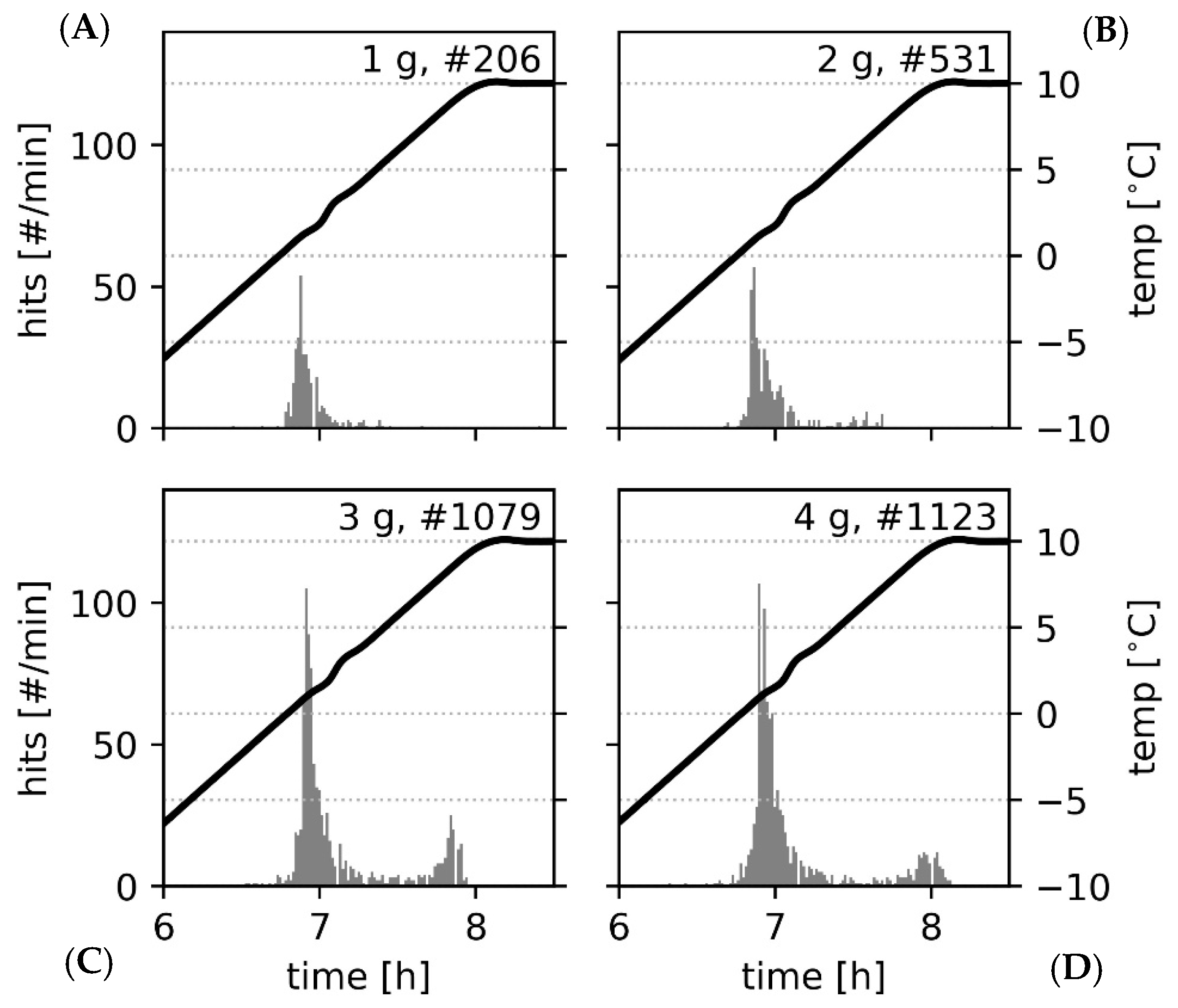
The gray histograms in Figure 4 show the number of acoustic signals during the melting of a water sample with different weights between $\mathrm{m}=1.0\pm 0.1$ $\mathrm{g}$ and $\mathrm{m}=4.0\pm 0.1$ $\mathrm{g}$. The black lines show the air temperature in the isolated box.

All four histograms show a high acoustic activity when the temperature reaches the melting temperature. Two peaks of acoustic activity can be identified. The first peak appears at the beginning of the melting process where the Celsius temperature just reaches a positive value. After an “activity valley”, another, lower peak appears at the end of the melting phase.

Prior to the increase of temperature in Figure 4 at $t<6\mathrm{h}$, the temperature is constant for approximately two hours. This time included, none of the performed measurements show more than five detected events until the temperature reaches $T\approx -2.5{}^{\circ }\mathrm{C}$.

The temperature curve confirms the reliable performance of the temperature controlling facility. The experimental setup reaches the target temperature within its limits and stabilizes the temperature at the lower plateau at $T=-14.00\pm 0.05$ ${}^{\circ }\mathrm{C}$. Taking a possible systematic offset from the NTC sensor into account, an air temperature uncertainty of less than $\Delta T=0.1\mathrm{K}$ can be assumed. During the constant raise of target temperature, the temperature shows a small variation of about $\Delta T\sim 30\mathrm{m}\mathrm{K}$ around the target temperature at $t\sim 7\mathrm{h}$. The registered time-dependent power that drives the Peltier-cooling element confirms this fluctuation around the constantly rising target temperature (not shown in Figure 4). Both can be explained with the latent heat of the melting process which results an additional “energy consumption” in the system. The temperature control unit reacts with a certain delay to this, which results in a slower temperature increase. This is followed by an “over-steering” of the temperature control unit and an increase of the temperature above the target temperature. In the upper right corner of each plot, the mass of water and total sum of acoustic events is indicated.

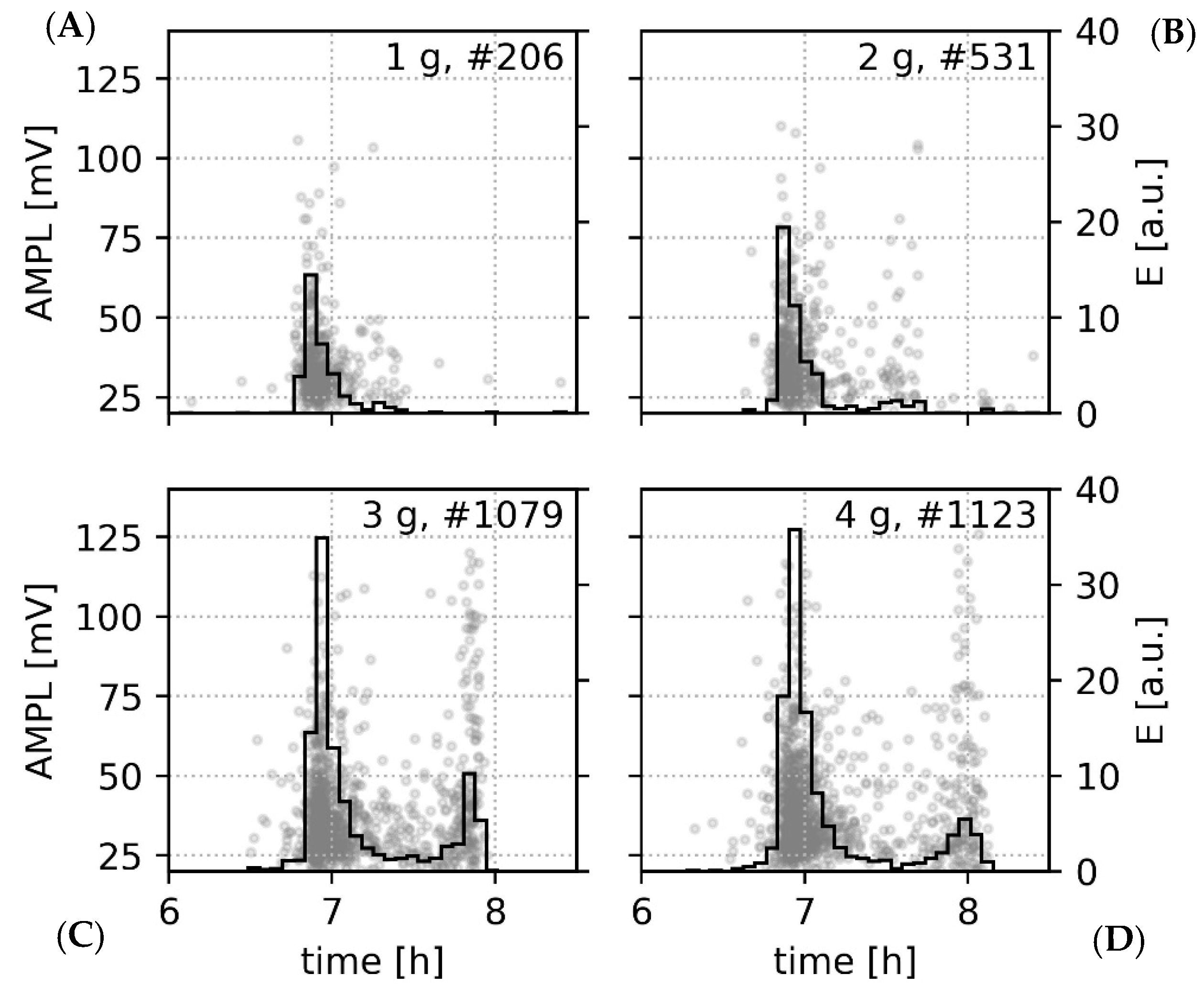
As described in Section 2.1, common AE parameters such as AMPL, D, RT and E are calculated for each acoustic event. This allows a later filtering and detailed parameter-based analysis. However, in this experiment, only the RT was used to distinguish between AE signal from the ice-melting and background noise. For this, a RT-filter with a threshold of RT $\ge 0.1$ $\mathrm{ms}$ was implemented. A different representation of the data can be seen in Figure 5 where all detected AE events are plotted in a scatter plot showing their AMPL and the time of occurrence (gray dots). The histograms in Figure 5 show the accumulated energy per time unit during the melting (black line). The single events, as well as the histograms which are very similar to the histograms in Figure 5 indicate that there is no significant change in the AMPL or acoustic energy of the events along the melting process. Also, the other parameters (D, RT) that are implicitly influencing the acoustic energy do not show any significant change during the melting process.

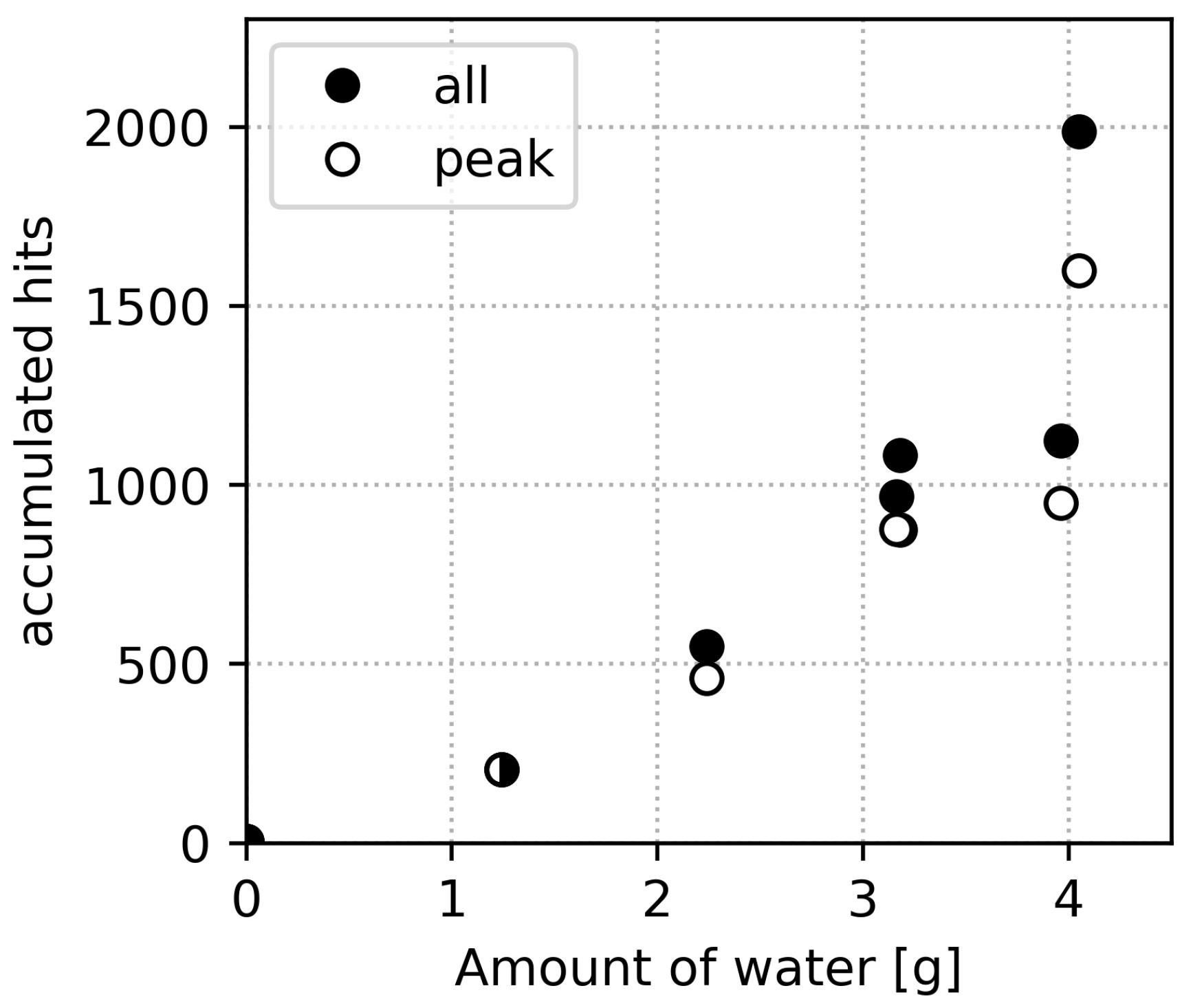
Figure 6 shows the acoustic activity during the melting of different samples with varying water quantities. The solid markers indicate the number of events measured during the complete melting process. As seen in Figure 4, the AE events in the initial melting phase dominate the total number of AE events. For the further analysis, the time between the two peaks divide the histograms in two parts (“first peak”, “second peak”). Besides all events (“all” = “first peak”+“second peak”), the number of events in the first peak (“peak”) are separately plotted in Figure 6 as circles. Only the missing “second peak” the measurement with the smallest quantity makes this distinction impossible and it is assumed that all AE events are in the “first peak”.

The usage of a weight scale reduces the uncertainty of the quantity of water per measurement that is assumed to be below $\Delta m_{ice}<0.1\mathrm{g}$.

4. Discussion

The measurements presented above show that the AE technique can monitor melting processes of ice quantitatively as well as qualitatively. The acoustic activity of ice in an environment with a constantly increasing temperature starts when the temperature reaches the melting temperature of water. Independent of the amount of water, the acoustic activity is the highest at the beginning of the melting process where rates of up to 125 AE events per minute where measured with the described setup. This number is however strongly dependent on the physical measurement setup, used hardware and signal filters.

Wentzell et al. [13] already reported a peak in the acoustic activity at the beginning of the melting process of ice. They identified the temperature gradient between the surrounding and the frozen sample as a root cause for crystal fractures that cause this peak. In the presented work, the very slow temperature increase ($\Delta T_{\uparrow }=8\mathrm{K}{\mathrm{h}}^{-1}$) prevents high temperature gradients within the sample and crystal fractures should not be a relevant source of acoustic events.

After this peak, the rate of the acoustic events decreases and a “valley” with significantly lower AE activity appears. For the measurements with amounts of water $m_{ice}>2.0\mathrm{g}$, the acoustic activity again increases towards the end of the melting process.

This behavior can have multiple reasons that include phenomena related to the intrinsic acoustic activity during the melting process or the acoustic coupling between source and sensor.

In Figure 7 a schematic, simplified of the temporal histogram of AE events during the melting process is shown and divided into three parts (A, B, C) that might correspond to different situations inside the sample holder.

During the first part of the melting (A), the sample is dominated by ice. At a certain point in time, the constantly increasing temperature results in the melting of ice and stress in the crystal due to the sudden change in volume during the melting. Therefore, a significant amount of acoustic energy is released in this initial stage. As seen in Figure 6, the number of acoustic events at the beginning of the melting process is dominated by the first peak and linear dependent on the amount of ice.

After the first peak, the acoustic activity decreases and the second phase (B) with less acoustic activity sets in. Therefore, the coupling of the AE source (melting ice) and the sensor changes. An additional film of water between the sensor and the ice results in an additional surface that reflects a part of the acoustic energy.

Finally, as described above and seen in all additional measurements, a remarkable increase of observed acoustic activity is measured at the end of the melting process. In this phase (C), only a little ice amount is left swimming at the surface of the water reservoir. This ice is therefore in contact with the air which is warmer than the water in the sample holder resulting in a higher temperature gradient. This could be one reason for a higher melting rate of the last bits of ice resulting in an increase of the acoustic activity.

To investigate this effect, measurements with a bucket that was closed with a cover and some vacuum grease were done. In this case, the air inside the bucket was trapped and not interchangeable with the external air. Therefore, it can be assumed that the effect of the ice touching “warm” air was reduced. However, also these measurements show the three phases of melting including the second peak at the end of the melting phase which suggests that the ice touching the “warm” air has no or only a minor effect.

5. Conclusions

The presented work shows that AE can monitor the melting process of ice which is accompanied by acoustic signals observed in the ultrasonic frequency range above 30 $\mathrm{k}$$\mathrm{Hz}$.

To conduct measurements in a controlled environment, an actively temperature-controlled box which can be heated and cooled with Peltier elements was build. With this, measurements on melting processes of different amounts of tap water were conducted. Basic signal analysis based on the time of occurrence, amplitude and length of acoustic events enables the monitoring of the melting processes. A systematic pattern of acoustic activity during the melting process with two peaks was measured. Due to these two peaks, which occur at the beginning and the end of the melting phase, the start, as well as the end of the melting, can be clearly estimated. In addition to this, the number of acoustic events in the first peak seems to be correlated with the amount of ice. These results show that AE can monitor melting processes in systems with a good acoustic coupling between the AE sensor and the melting ice. This is especially interesting when melting ice must be identified in areas which are difficult to access, as for instance a fuel tank within an aircraft during the daily maintenance. Here, information about ice in the fuel tank would improve the safety and efficiency of draining processes which remove liquid water from the tanks in the hangar.

6. Outlook

The presented work shows that melting of ice can be monitored with AE. However, in this work only very little information (time of occurrence, AMPL, E, D, RT) were deduced from the acoustic signals and no spectral analysis was performed yet. Thus, additional information that can be deduced from a spectral analysis with well-known methods such as modal analysis or principal component analysis as done by Surgeon and Wevers [20], Johnson [21] respectively. One question is if the two peaks in the histogram originate from different physical phenomena during the melting and if a detailed spectral analysis can differentiate the signals in the first and second peak. However, for this, it must be ensured that the spectral composition of the acoustic transients is not heavily influenced by the experimental setup and the changing physical properties of the sample during each measurement.

In addition, the influence of physical parameters such as the cooling rate during the freezing, the purity of the sample and related freezing temperature and chemical composition of the sample to the acoustic activity have to be investigated. For this, a temperature measurement inside the ice/water mixture during the experiment would provide further insights into the freezing/melting behavior of the sample. Combined with repetitive measurements of the same setting and resulting statistics, fundamental properties of the sample could be derived only by recording and analyzing the acoustic signals during the melting.