A Multi-Branch-and-Bound Binary Parallel Algorithm to Solve the Knapsack Problem 0–1 in a Multicore Cluster

Featured Application

An uncorrelated instance is equivalent to solving any problem where the benefit is independent of the weight. A weakly correlated instance has a high correlation between the benefit and the weight of each element. Typically, the benefit differs from the weight by a small percentage. Such instances are the most practical in administration, such as with a return on an investment, which is generally proportional to the sum of the amount invested.

Abstract

This paper presents a process that is based on sets of parts, where elements are fixed and removed to form different binary branch-and-bound (BB) trees, which in turn are used to build a parallel algorithm called “multi-BB”. These sequential and parallel algorithms calculate the exact solution for the 0–1 knapsack problem. The sequential algorithm solves the instances published by other researchers (and the proposals by Pisinger) to solve the not-so-complex (uncorrelated) class and some problems of the medium-complex (weakly correlated) class. The parallel algorithm solves the problems that cannot be solved with the sequential algorithm of the weakly correlated class in a cluster of multicore processors. The multi-branch-and-bound algorithms obtained parallel efficiencies of approximately 75%, but in some cases, it was possible to obtain a superlinear speedup.

1. Introduction

The KP 0–1 (knapsack problem 0–1) has a wide variety of applications in everyday life, including production planning, financial modeling, project selection, the allocation of data in distributed systems, and facility capacity planning [1].

Due to the diversity of real problems, it is necessary to consider them through problem models, such as those proposed by Reference [2]. They proposed seven classes of problems, and we focused on solving two of them in this work: the uncorrelated and the weakly correlated. Uncorrelated problems model any problem in which the weights of the elements are not correlated with their benefit. The weakly correlated problem model offers many practical applications, such as capital budgeting, project selection, resource allocation, cutting stock, and investment decision-making [3]. In this way, if an algorithm performs well in solving these instances, it is likely to solve a problem in everyday life.

The characteristic of this problem is that its items cannot be split among themselves and is classified as an NP-hard problem, where NP, indicates non-polynomial behavior problems. For certain sizes of the instances of these problems, it is possible to calculate their optimal solution by means of algorithms and parallel computers. Therefore, a parallel BB (Branch and Bound) algorithm is proposed to calculate the exact solution of KP 0–1 for instances of medium and low complexity (weak and uncorrelated [2], respectively).

The novelty of this work is that using a different approach to a binary tree (from a formulation of a set of parts), we propose generating several different trees to find the optimal solution [4,5,6,7,8,9,10]. Each of these trees represents a decision tree that is generated by fixing or removing elements, so the roots of these trees are located in different search spaces with respect to the initial tree. Each binary tree forms new search spaces, and consequently there are a greater number of feasible solutions available. Because each decision tree is independent of the others, each of them is assigned in a processing unit for execution, and therefore it is possible to calculate the optimal solution more quickly and thus reduce the computation time, sometimes determining superlinear speedup as well as solving the instances that cannot be resolved with a sequential approach.

The factors involved in efficient parallel implementation are diverse: those corresponding to the algorithm and those inherent in the use of parallel computers. It is important to consider algorithms that are efficiently parallelizable, i.e., algorithms whose execution times are polylogarithmic and use a number of polynomial processors (both depending on the size of the input) [11]. However, in the parallel BB algorithms applied to solve the integer knapsack problem and its version, 0–1, additional variables were used to express complexity, such as the capacity of the knapsack $c$ and the weights of the elements (the maximum $w_{max}$ and the minimum $w_{min}$ [12]). This indicates that these variables influence the complexity of the instance and, consequently, its execution time.

On the other hand, the factors that influence the performance of the parallel implementation of the BB are shared knowledge, knowledge use, division of work, and synchronization. These are considered independently of the computer architecture and the BB parallel algorithm to solve KP 0–1 [13].

In different parallel BB algorithms and their implementation in multicore computer architectures and GPUs (Graphics Processing Units), two points of view are considered: developing a parallel algorithm and the factors that influence that algorithm’s implementation [14,15]. This paper proposes a way to search for the optimal solution from an algorithmic point of view, generating greater spaces with feasible solutions and their implementation in a multicore cluster.

In BB parallel models, a decision tree travels through the space of feasible solutions until reaching the optimum [14,15,16]. That is to say, collectively, a single tree is crossed until reaching the optimal solution. In our BB parallel model, we propose generating several different trees to find the optimal solution [4,5,6,7,8,9,10]. Each of these trees represents a decision that is generated by fixing or removing elements, so the roots of these trees are located in different search spaces with respect to the initial tree. The implementation of this algorithm was performed in the multicore cluster “Ioevolution”, with 136 cores distributed among four servers.

The sequential algorithm solves all the uncorrelated instances, and our algorithm, the “multi-BB” solves all of the weakly correlated instances, with superlinear speedup found in some solutions.

The formulation of the KP 0–1 and related works are discussed in Section 2. In Section 3, we describe the hypotheses of our work and the procedure to generate the decision trees. The implementation and testing are done in Section 4, as is a discussion of the results. In Section 5, we present the conclusions of this paper.

2. Foundation

2.1. Problem Formulation

The 0–1 knapsack problem has been among the most studied problems in the literature since 1897 [17]. The mathematician Tobias Dantzig named the problem in the early 20th century [18]. Its formulation is simple, but its solution turns out to be complex, since it is a problem that grows exponentially. Therefore, in the theory of complexity, KP 0–1 is classified as an NP problem [19].

The 0–1 knapsack problem arises as follows:

$$f_{opt}=max{\sum }_{i=1}^n{p}_i{x}_i,$$

(1)

subject to

$${\sum }_{i=1}^n{w}_i{x}_i\le c,$$

(2)

where $f_{opt}=$ optimal function; $p_i=$ element benefit $i, p_i\in Z^{+}$; $w_i=$ element weight $i, w_i\in Z^{+}$; $c=$ knapsack capacity, $c\le {\sum }_{i=1}^n{w}_i$; and $x_i=$ element $x_i\in \left\{0,1\right\}$.

The formula in Equation (1) refers to maximizing the utility of the knapsack based on the sum of the benefits of each of its elements. This restriction indicates that it is necessary to take into account the sum of the weights of the items that will be stored in the knapsack, whose capacity is determined by the variable $c$. The variable $x_i$ is “0” when the item is not included in the knapsack and “1” when the item is included.

The KP 0–1 consists of determining the elements that should be included in the knapsack, so the total utility of the selected elements is maximum, without exceeding the allowed capacity of the knapsack.

2.2. Related Works

The BB parallel algorithms used to solve KP 0–1 have been designed primarily for static computer architectures, such as rings, toroids, and hypercubes [12]. Subsequently, these algorithms have been implemented in dynamic configuration computers, multicore CPUs (Central Processing Units), and GPUs [14,15], where the focus is mainly on the four factors that influence implementation: shared knowledge, knowledge utilization, division of work, and synchronization [13].

The complexity of the BB parallel algorithms that solve the KP 0–1 is a function of the problem instance variables. For example, when the computer architecture is a hypercube, the complexity is given by [12,15]

$$O\left(\frac{nc}{p}\frac{w_{max}}{w_{min}}\right)$$

(3)

for a number of processors of $p<\frac{c}{\log w_{max}}$.

In Equation (3), one of the terms is $\left(\frac{w_{max}}{w_{min}}\right)$. If this term grows, then the complexity increases, unlike the classification proposed by Martello et al. [20], where the complexity of KP 0–1 is given by the variability of the benefit with respect to the weights of the elements ($p_i$ and $w_i$). Martello et al. [20] classified the complexity of KP 0–1 into seven different instances grouped into three complexities based on the correlation between the $p_i$ benefit and the weight $w_i$ [2]. The equations for three of the seven representative instances of each of the complexity classes are shown below:

$$\mathrm{not}\mathrm{correlated}:w_i\in \left[1, R\right] and p_i\in \left[1,R\right];$$

(4)

$$\mathrm{weakly}\mathrm{correlated}:\hspace{1em}{w}_i\in \left[1,R\right] and p_i\in \left[w_i-\frac{1}{10}R, w_i+\frac{1}{10}R\right]\mathrm{such}\mathrm{that} p_i\ge 1;$$

(5)

$$\mathrm{strongly} \mathrm{correlated}:\hspace{1em} w_i\in \left[1, R\right] and p_i=w_i+\frac{1}{10}R;$$

(6)

where $p_i=$ the benefit of element $i$; $w_i=$ element weight $i$; and $R\in \left\{1,000,10,000\right\}$.

As observed in the previous equations, the complexity of the instance is not only given by the variability of the weights of the elements $\left(w_i\right)$, because the elements are calculated in the same way in the three instances. Therefore, the increase in complexity is given by the variability of the benefit of the elements $p_i$ with respect to $w_i$.

The other term of Equation (3), $\left(\frac{nc}{p}\right),$ indicates that the capacity of the knapsack is important in determining the execution time of the algorithm. This coincides with the results of various researchers [2,14], who determined that the capacity of the knapsack affects complexity, so the tests are carried out by varying the capacity of the knapsack or half of the sum of the weights of the elements.

In recent implementations in multicore computer architectures and GPUs [14,15,16], the focus has been on the four factors identified by Trienekens and de Bruin [13], as well as on using the two search criteria in combination: the first is depth, and the second is breadth [15]. With depth, the tree levels are advanced, and with breadth, the volume of subproblems is generated to use massive computation. However, the search remains for a single decision tree. Once the volume of children is generated to use these architectures, scholars have focused on developing an algorithm that considers the following:

• Shared knowledge: this consists of the list or lists of the subproblems or nodes that are stored for later calculation and divided in two (the type of storage of the subproblems (general or local) and how that list is updated);
• Knowledge use: This is divided in two (the access strategy for the list of subproblems and whether that knowledge is shared with the results) and is updated immediately (the optimal solution and limits);
• Division of work: This is formed by the active processes. In this way, the unit of work in each process and the load balance are determined;
• Synchronization: This refers to the synchronization of each of the concurrent processes for data communication.

3. Proposed Model

3.1. Considerations for the Elaboration of the Parallel Algorithm

Our model starts from a sequential algorithm that has been previously described in Reference [21], to which some improvements and modifications were made to elaborate on the parallel algorithm.

The search space for the discrete knapsack problem 0–1 is given by the power set of the elements of the initial problem. If these elements are in the set $I=\left\{1,2,\dots ,m\right\},$ then the number of subsets of the power set or parts is |P(I)| = 2^m. The power set can be represented using the terms of the empty set ϕ and the set I, whereby the power set can be denoted by P (m) = [ϕ, I]. If the fixed elements are in the set ${\omega }_1$, and the elements assigned to the node are in the set ${\omega }_2$, then P(m) can also be denoted by P(m) $=\left[{\omega }_1,{\omega }_2\right]$ [22,23].

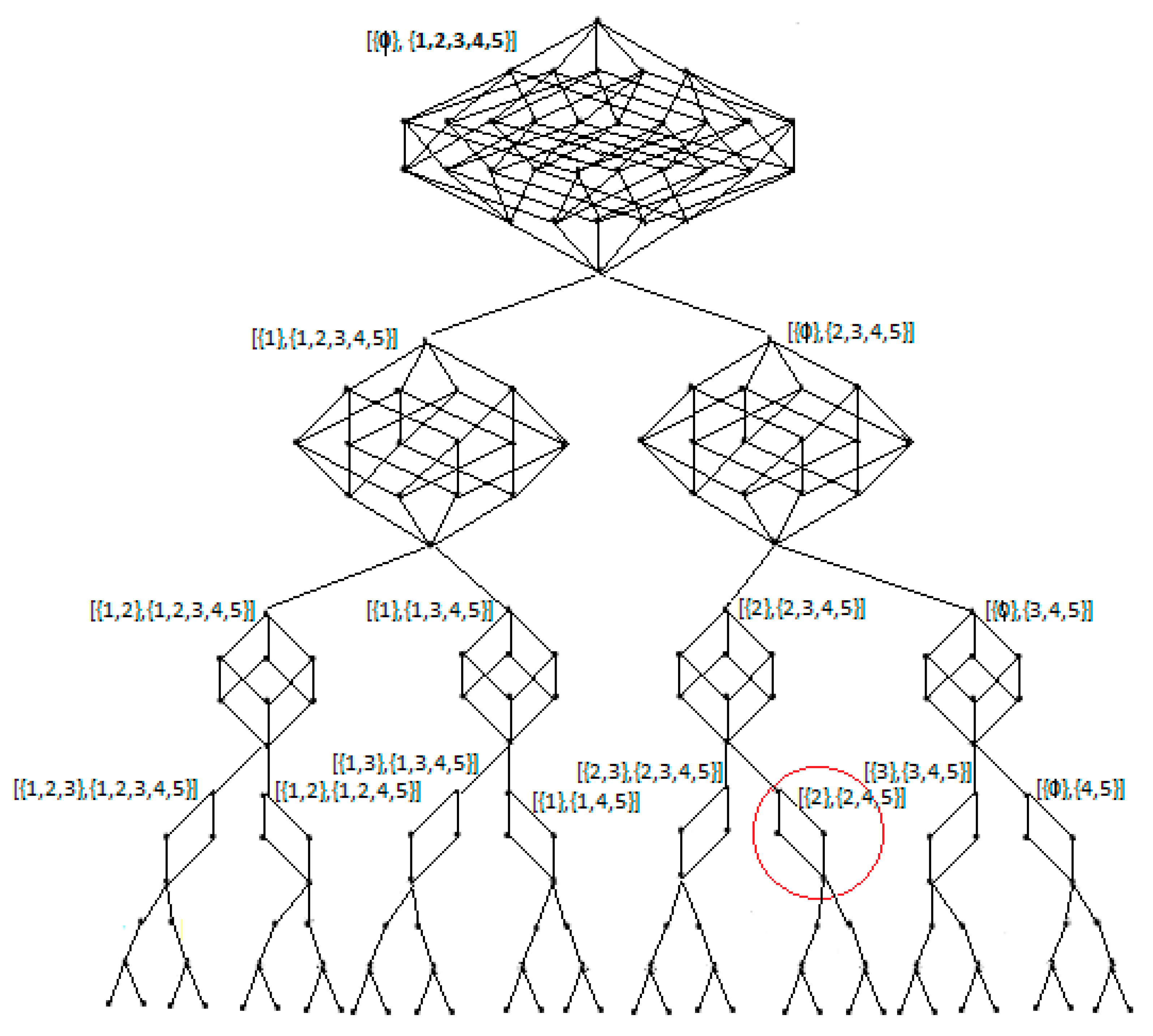
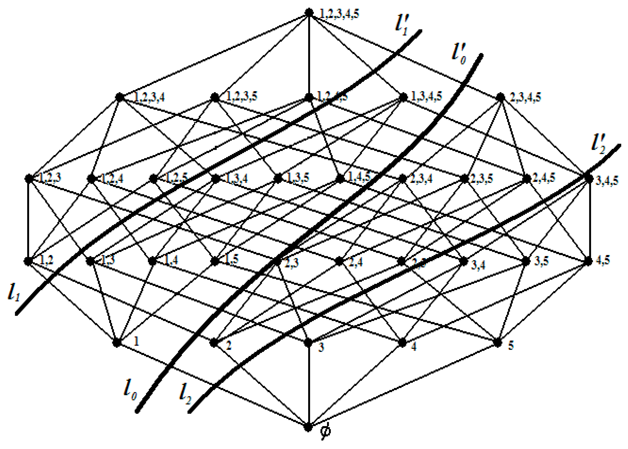
An example of the initial search space of a KP 0–1 with five elements is shown in Figure 1. The search space is for set $I=\left\{1,2,3,4,5\right\}$.

This space is divided into two when an item is fixed or removed. In Figure 1, the line $l_0{l}_0^{\prime }$ divides the search space in two by setting and removing element 1: the left side is the left child and the right side is the right child. As can be seen in Figure 1, the search space of the left child consists of all the subsets containing element 1. On the other hand, in the search space of the right child, no subset has element 1 as its element. These two spaces correspond to level 1 of the binary tree, as shown in Figure 2.

In turn, these search spaces are divided in two by setting and removing element 2. The line $l_1{l}_1^{\prime }$ shows the spaces generated with the left child, and line $l_2{l}_2^{\prime }$ shows the spaces generated with the right child. Therefore, at level 2, there will be four nodes. Each of these children is divided into two sets whose search space is a smaller dimension than the search space of the node from which they come. There are two sets of level 3 for each of the sets of level 2. In level 3, there will be eight sets. In general, at the level of $k, 0\le k\le m, 2^k$, subsets can be formed, where the search spaces of every two sets are disjointed sets and the union of all spaces of the same level is the initial power set P(m). Following this procedure, at the last level, a subset of the initial power set is assigned to each leaf [25].

In the last levels of the binary tree, most of the elements will be fixed at ω₁, leaving a small number of free elements. Taking into account the above, the KP 0–1 is formulated below:

$$\begin{array}{c}{f}_{opt}=max\left[\begin{array}{ccc}{\sum }_{i\in {\omega }_1}{p}_i& +& {\sum }_{i\in \left({\omega }_2/{\omega }_1\right)}{p}_i{x}_i\\ {\sum }_{i\in {\omega }_1}{w}_i& +& {\sum }_{i\in \left({\omega }_2/{\omega }_1\right)}{w}_i{x}_i\le c\\ x_i\in \left\{0,1\right\}& for& i\in I\end{array}\right],\\ c=\lambda C\end{array}$$

(7)

$$C={\sum }_{i=1}^n{w}_i,$$

(8)

$$0\le \lambda \le 1, w_i ,p_i\in Z^{+}$$

where $p_i$ is the benefit of element $i, w_i$ is the element weight i, and $c$ is the knapsack capacity.

Equation (7) is divided into two terms: fixed $\left({\omega }_1\right)$ and free elements $\left({\omega }_2/{\omega }_1\right)$. Therefore, the formulation of the problem is adapted to the part of the problem that contains free elements: this is because it is not known which of them will be part of the solution. The modification consists of calculating the capacity of the available knapsack, once the fixed elements have been stored in the knapsack, according to Equation (9):

$$c_0=c-{\displaystyle \sum }_{i\in {\omega }_1}{w}_i.$$

(9)

This algorithm begins with the calculation of a feasible solution and its upper and lower limits: these are obtained as proposed by Dantzig (1957) [18] with Equation (10). The algorithm calculates them only once at the beginning of the calculations:

$$\frac{p_{i_1}}{w_{i_1}}\ge \frac{p_{i_2}}{w_{i_2}}\ge \dots \ge \frac{p_{i_n}}{w_{i_n}}.$$

(10)

Subsequently, for free items $\left({\omega }_2/{\omega }_1\right)$, the critical variable x_s is determined by Equation (11), the upper bound (UB) limit by Equation (12), and the lower bound (LB) limit by Equation (13), where the LB will be the first optimal integer solution (f_opt):

$$x_s=min\left\{l_0:{\sum }_{i_k=1}^{l_0}{w}_{i_k}>c_0\right\},$$

(11)

$$UB=\left[LB+\left(c_0-{\sum }_{i_k=1}^{l_0-1}{w}_{i_k}\right)\frac{p_{i_0}}{w_{i_0}}\right],$$

(12)

$$LB={\sum }_{i\in {\omega }_1}{p}_i+{\sum }_{i_k=1}^{l_0-1}{p}_{i_k},$$

(13)

where $c_0$ is the available capacity of the knapsack that will be filled with free items $\left({\omega }_2/{\omega }_1\right)$, $l_0$ is the minimum number of free elements that cause the sum of the weights $w_i$ to be greater than $c_0$, p_i is the benefit of the critical element, and $w_i$ is the weight of that critical element.

After determining the critical variable and the root limits ($UB$ and $LB$), two children are generated using the procedure described previously, and each of the children will have a $U{B}_{child}$ that is used to determine if that child is pruned or branched. In order for the child to branch out, the following must be fulfilled:

$$U{B}_{child}>f_{opt}.$$

(14)

If Equation (14) is met, there is a possible $L{B}_{child}$ that is better than the current one and, consequently, a better optimal solution if $L{B}_{child}>f_{opt}$. On the other hand, if $U{B}_{child}<f_{opt}$, then that branch of the tree is pruned, since there will be no $L{B}_{child}$ greater than the best $f_{opt}$ that has so far been calculated. The optimal solution $f_{opt}$ is the control variable.

3.2. Multi-BB Parallel Model

The sequential BB algorithm uses a breadth search to traverse the binary tree and calculate the optimal solution. This algorithm progresses level by level, calculating all the subsets generated. Therefore, to explain the proposal of the parallel model, the following example is presented. The subset {2, 4} is supposed to be the optimal solution to the problem. The subset {2, 4, 5} is at level 3, as is shown in the tree in Figure 2, where elements 2 and 4 are in the first locations. Thus, the algorithm will have to reach level 3 to calculate the solution. In the worst case, the algorithm will require 2⁰ + 2¹ +2² + 2³ subsets, so it will also be necessary to perform calculus for the subsets of level 4 (2⁴) to determine that the solution is optimal. These subsets are stored in a list and are resolved sequentially. In the worst case, the calculated subsets will be 31.

When at the start of the problem, element 3 is fixed and removed instead of 1, the subsets by level are level 0 [ϕ, {1,2,3,4,5}]; level 1 [{3}, {1,2,3,4,5}] and [ϕ, {1,2,4,5}]; and level 2 [{1,3}, {1,2,3,4,5}], [{3}, {2,3,4,5}], [{1}, {1,2,4,5}], and [ϕ, {2,4,5}]. The solution is in the last subset. The number of subsets needed to reach the solution is 2⁰ + 2¹ + 2², and the subsets of level 3 (2³) will be required to determine that the solution is optimal. In the worst case, 15 subsets will be calculated, which is 2⁴ operations less than in the previous case.

Because the fixed or removed element that helps determine the optimal solution in fewer iterations is not known in advance, we propose generating different binary trees. In each tree, a different element is fixed or removed. When the element is fixed, that element is forced to be part of the solution, and when it is removed in another tree, that element will not be part of the solution, meaning that other elements must form the solution. In each binary tree, the process described previously is followed. The processing units share their best solution to accelerate the calculation, thereby increasing the number of branches that are pruned in each tree. Consequently, it is possible to reduce the parallel computation time. Communications among the processing units influence the synchronization of the processing units, an aspect that is resolved, as indicated in the following paragraphs. The ideal number of binary trees is equal to twice the number of elements of the problem, because in one-half of the trees, a different element is fixed, and in the other half, each element is removed.

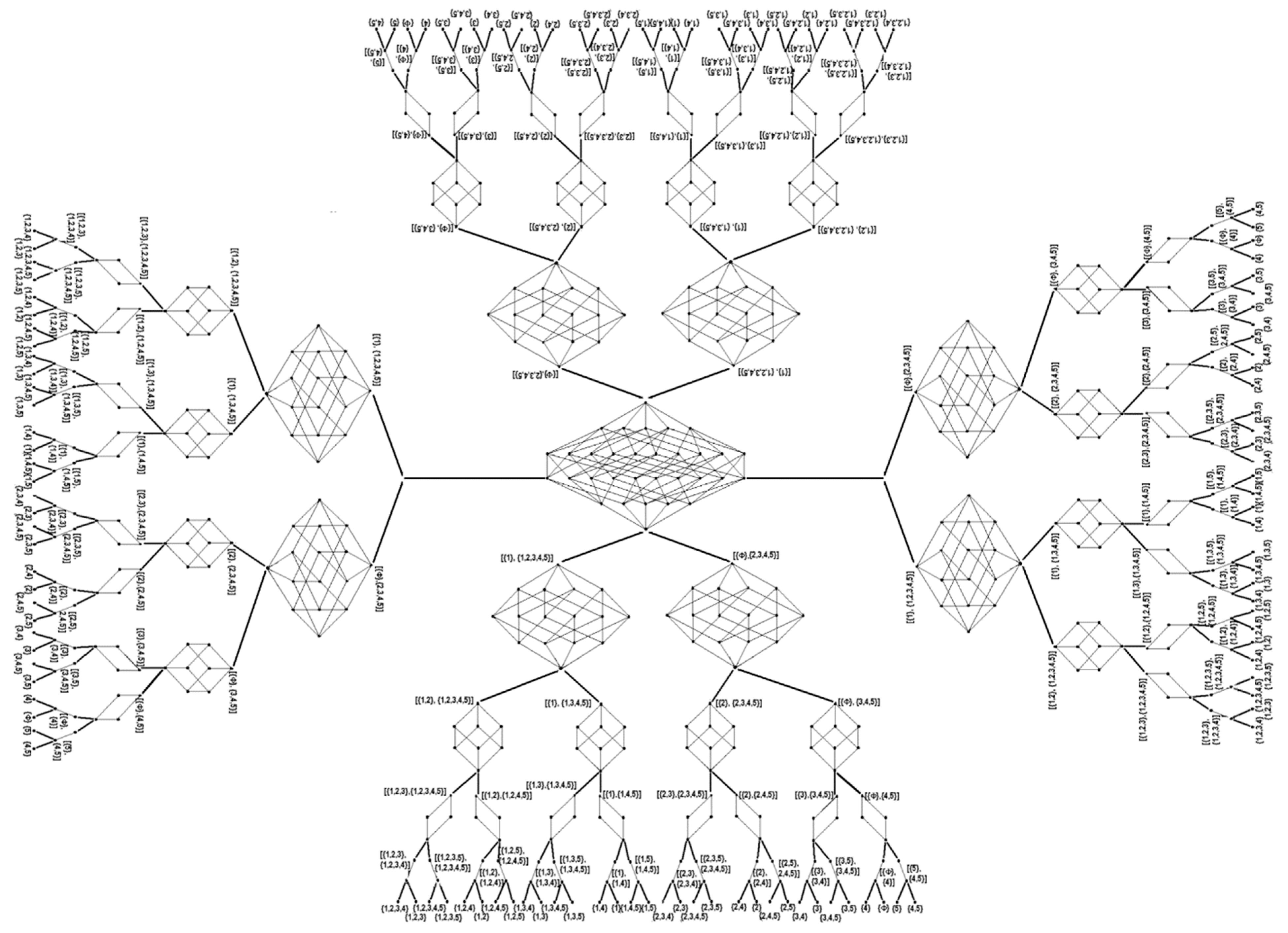
Therefore, we propose generating different trees to increase the spaces of the feasible solutions, with the possibility that in some binary trees, the optimal solution is found in its first levels.

An outline of the algorithm is shown in Figure 3, where the trees that are generated do not constitute a forest [24] because they share the same leaves.

3.3. Multi-BB Algorithm for a Multicore Cluster

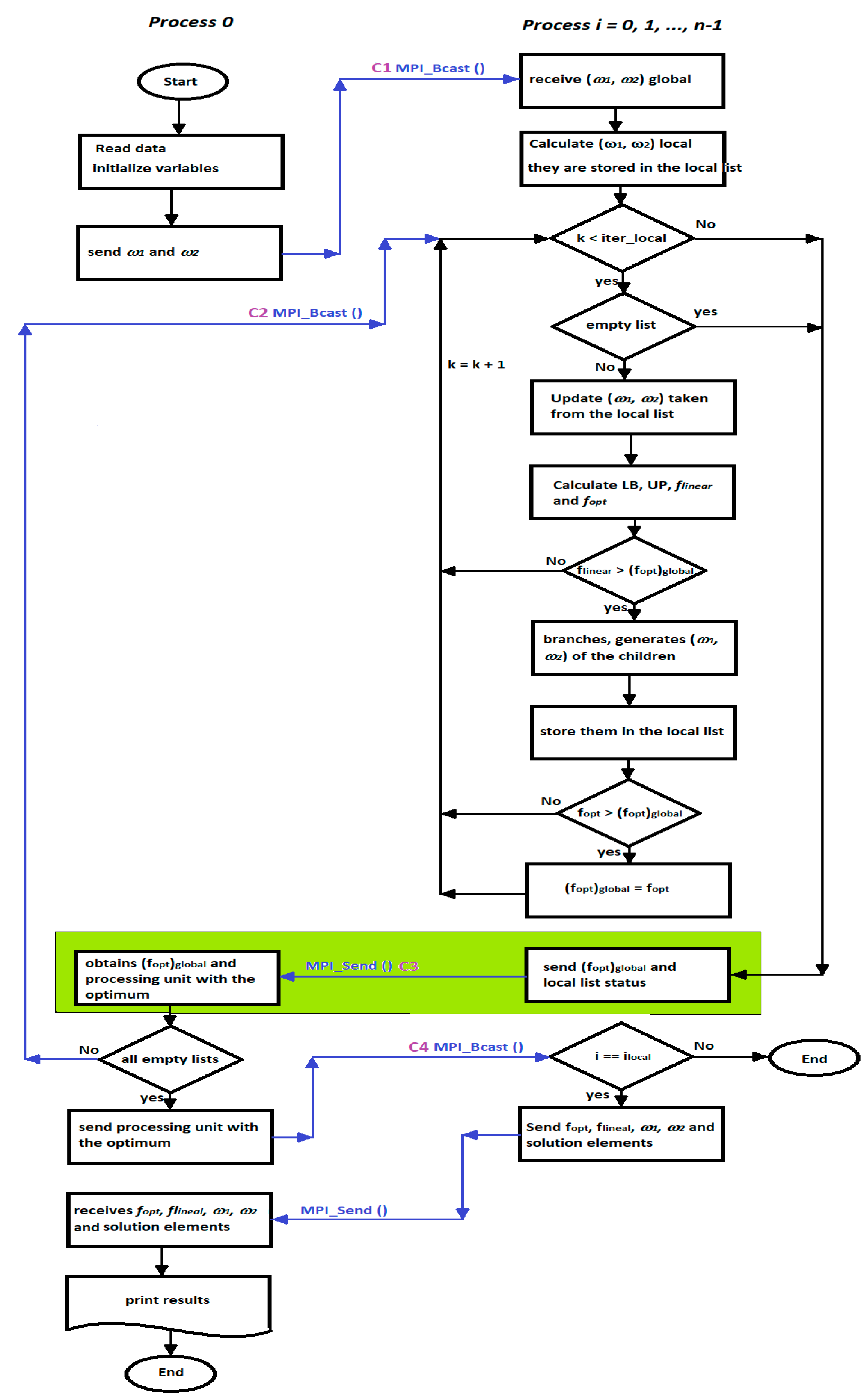
In the implementation of the multi-BB algorithm in the multicore cluster (Figure 4), four factors that influence its efficiency are considered: shared knowledge, knowledge utilization, work division, and synchronization [13]. These are defined to have a good load balance, a minimum number of synchronization points, and the shortest communications times.

Shared knowledge, or the subsets that are generated by the branching of trees, is stored in local lists in each processing unit because each of the multi-BB trees is independent of the others. An Exclusive Read, Exclusive Write, Parallel Random Access Machine (EREW PRAM) model is used for access to the subsets and to write the partial solution. Figure 4 shows how the local lists are used in each processing unit, from how they are started and updated to when the subsets are taken.

For division of the work, both in a static form and at the beginning of the calculation, a tree is assigned to each processing unit. Each decision tree is expected to grow, and a good load balance is achieved. This is the first activity that the processes perform, as is seen in Figure 4.

With regard to the use of knowledge and synchronization, the optimal solution is shared knowledge. The processing units are synchronized to exchange partial solutions and determine the optimal solution to the problem. A processing unit receives partial solutions, obtains the optimal solution, and stores the identification of the processing unit within that solution. The above process is presented in a green box in Figure 4. The number of local iterations to carry out the synchronization is based on the proposal by Zavala-Díaz [24].

The algorithm is asynchronous when each processing unit travels through its search space. Synchronization occurs when the processes send and receive information (blue lines in Figure 4). Communications C1, C4, and C5 are executed only once during the entire calculation process. In communication C1, the elements in ${\omega }_1$ and ${\omega }_2$ of the problem are sent. In communication C4, the master processor sends data to all others and the number of the processing unit that calculated the optimal solution. In communication C5, the processing unit with the optimal solution sends the data to the master processor of the optimal solution, such as ${\omega }_1$,${\omega }_2$ (the set of solution elements for $f_{linear}$ and $f_{opt}$). Communications C2 and C3 are made each time the maximum number of local iterations is reached. In both cases, only two datapoints are sent. In communication C2, the master sends the updated global solution and the signal to the processing units to continue the calculations. In communication C3, each processing unit sends its $f_{opt}$ solution and the status of its local list.

The multi-BB algorithm was programmed in ANSI C, and the Message Passing Interface (MPI) library is used to pass messages. The number of maximum local iterations is one-tenth the size of the problem [24]. The proposed distribution for the parallel processes number is described in Section 4.2. The remaining variables have been previously described.

4. Computational Experimentation

Computational experimentation is divided into two parts. In the first part, the sequential algorithm is tested, the published instances are resolved, and the uncorrelated and weakly correlated instances are resolved. In the second part, the most complex instances found in the first section with the parallel algorithm are solved.

Table 1. Characteristics of the Ioevolution cluster.

Machines	Processor	Number of Processors	Cores per Processor	Cores Available
Ioevolution	Intel(R) Xeon (R) CPU @ 3.40 Ghz	8	4	32
compute-0–0	Intel(R) Xeon(R) CPU E5645 @ 2.40 Ghz	12	6	72
compute-0–1	Intel(R) Xeon(R) CPU X3430 @ 2.40 Ghz	4	4	16
compute-0–2	Intel(R) Xeon(R) CPU X3430 @ 2.40 Ghz	4	4	16
Total				136

shows the main characteristics of the Ioevolution cluster.

For a comparison between the results obtained with the sequential BB and parallel multi-BB algorithms, the following tests were carried out. In the first test, it was verified that the algorithm elaborated using sets of parts calculated the optimal solution. For this purpose, the optimal solution (based on the published instances with solutions) was calculated [26,27,28]. The second part consisted of solving the instances classified as uncorrelated and weakly correlated: their coefficients were given by equations as each author calculated them [14]. Therefore, it was not possible to directly compare these equations to other algorithms.

The sizes of the instances of our tests were similar to those used in other analyses: up to 50 elements [14] and up to 500 elements, with the size of the instances of 50 elements being frequent [29] (up to 2000 elements [16]).

4.1. Results of the Sequential Algorithm

Sequential execution was carried out on the Ioevolution server. To verify that the proposed method solved the knapsack problem 0–1, the instances published by References [26,27,28] were resolved.

Table 2. Tests of the instances from Reference [26].

Instance	Dimension	Knapsack Capacity	Optimal Solution Reference	${\mathit{f}}_{\mathit{o}\mathit{p}\mathit{t}}$
Kp_01	10	269	295	295
Kp_02	20	878	1024	1024
Kp_03	4	20	35	35
Kp_04	10	60	52	52
Kp_05	7	50	107	107
Kp_06	23	10,000	9767	9767
Kp_07	5	80	130	130
Kp_08	20	897	1025	1025

,

Table 3. Tests of the instances from Reference [27].

Instance	Dimension	Knapsack Capacity	Optimal Solution Reference	${\mathit{f}}_{\mathit{o}\mathit{p}\mathit{t}}$
Kp_01	4	100	473	473
Kp_02	10	100	798	798
Kp_03	25	300	3307	3307
Kp_04	40	600	4994	4994

and

Table 4. Tests of the instances from Reference [28].

Instance	Dimension	Knapsack Capacity	Optimal Solution Reference	${\mathit{f}}_{\mathit{o}\mathit{p}\mathit{t}}$
Kp_01	30	577	1437	1437
Kp_02	40	819	1821	1821
Kp_03	50	882	2448	2448
Kp_04	60	1006	2917	2917
Kp_05	65	1319	2818	2818

show the results obtained.

As can be seen in Table 2, Table 3 and Table 4, the sequential algorithm was capable of solving any simple instance. The importance of the comparison is in showing that the process of building ever-smaller solution spaces works to determine the optimal solution.

The second step was to resolve the instances of KP 0–1 that were classified as uncorrelated or weakly correlated. The tests were done with six sets of 1000 elements, for which the optimal solution for every 100 elements was calculated: n = 100, 200, …, 1000. In this way, the influence of the size of the problem could be measured, and it could be determined if the execution time depended on other variables. The value of the constant R was equal to 1000 for the first three series and was equal to 10,000 for the second three series. For each test, the capacity of the knapsack is given by Equation (15).

Table 5. Execution times of the uncorrelated instances.

Number of Elements	Time in Seconds
	Series 1	Series 2	Series 3	Series 4	Series 5	Series 6
100	0.04	0.02	0.03	0.03	0.01	0.02
200	0.13	0.32	0.14	0.55	0.21	0.31
300	0.26	0.86	0.22	1.38	0.41	0.73
400	0.34	4.29	0.25	2.79	3.77	10.59
500	3.1	2.8	2.7	8.81	4.92	17.29
600	11.26	6.55	11.65	10.9	33.61	7.16
700	17.64	31.02	9.44	24.43	54.52	21.3
800	109.58	260.64	105.71	124.82	14.08	44.93
900	196.51	18.51	279.35	311.9	25.2	68.39
1000	304.91	1127.53	25.6	132.39	474.34	72.61

and Figure 5 contain the sequential execution times for the uncorrelated instance problems:

$$c=0.5{\sum }_{i=1}^n{w}_i.$$

(15)

The results show that the sequential version calculated all of the series of uncorrelated instances. Table 5 and Figure 5 show that the runtime increment was primarily based on the size of the problem, tending to increase as the problem size increased. This increase was not linear (like the increase in the number of elements was), and in Figure 5, the vertical axis is presented in base logarithm 10. Only one of the results obtained had an execution time of more than 1000 s. This result was from series 2, with n = 1000. The values of this series were calculated with R = 1000, indicating that it is not practical to use R = 10,000 (in series 4, 5, and 6).

Table 6. Execution times of the weakly correlated instances.

Number of Elements	Time in Seconds
	Series 1	Series 2	Series 3	Series 4	Series 5	Series 6
100	0.19	0.13	0.21	0.24	0	0.05
200	12.04	1	11.85	2.73	0.17	0.69
300	178.49	2.78	153.05	3.66	76.77	6.82
400	67.03	26.75	61.77	13.8	9334.98	52.75
500	2751.75	710.1	2424.91	22.62	16.74	9.25
600	275.78	11.36	251.82	--------	43.34	46.11
700	5629.58	9017.98	352.74	32,133.68	151.03	177.34
800	640.93	1097.54	--------	-------	2063.79	47,107.17
900	--------	30.6	5.54	10,480.83	---------	---------
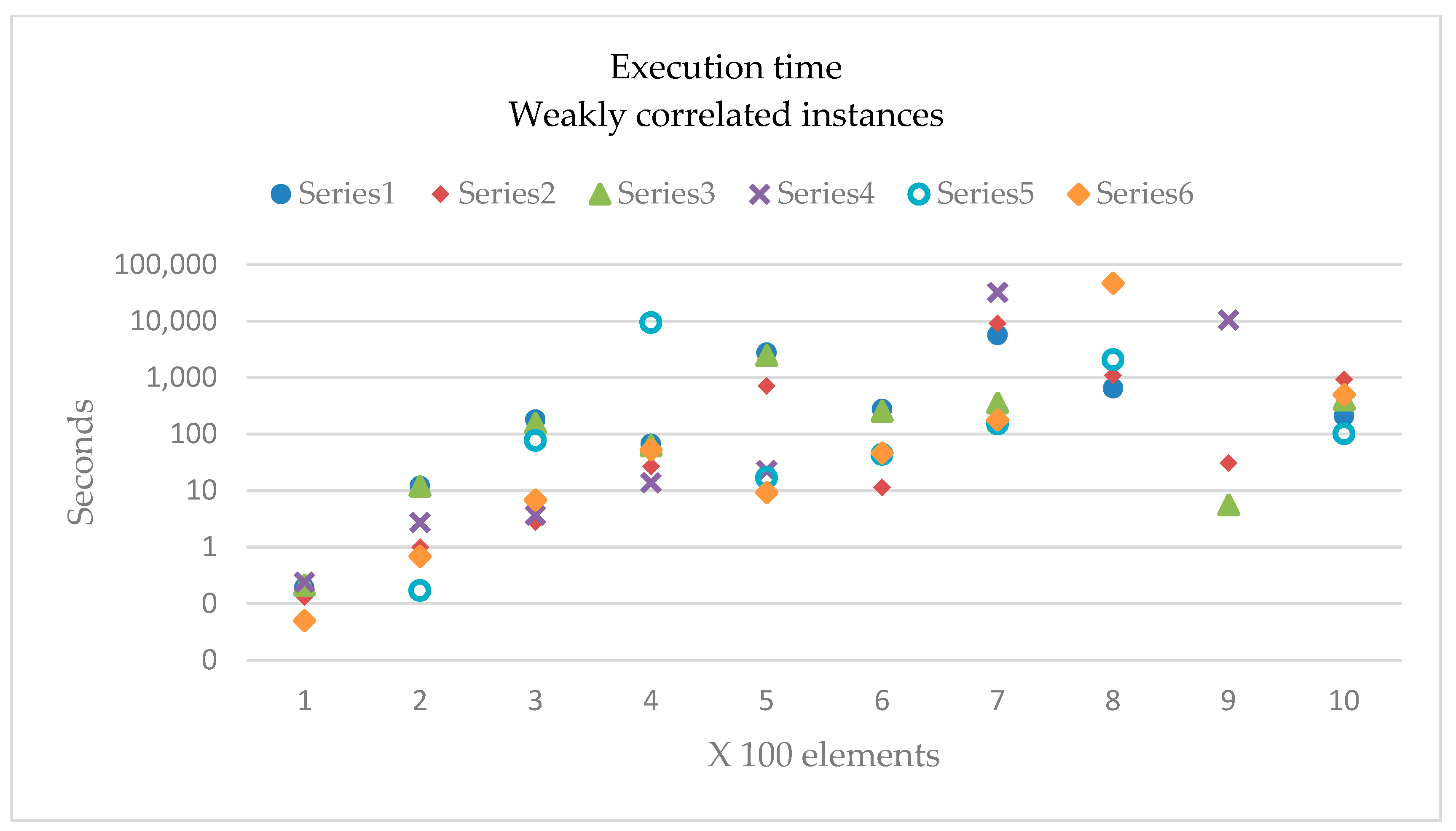
1000	207.47	923.5	400.23	-------	100.84	498.51

and Figure 6 show the sequential execution times for a weakly correlated instance.

With the sequential algorithm, it was not possible to obtain the optimal solution for all the problems in this instance. Seven of the sixty problems were not solved by the sequential algorithm, as shown in Table 6 and Figure 6. Some instances were not resolved because a number of generated children used all the memory of the Ioevolution server. Figure 6 shows that an increase in size influenced the execution time but also influenced the variability of p_i with respect to $w_i$, which caused a greater dispersion of execution times. The influence of using a constant R equal to 10,000 increases complexity in this kind of problem. Four of the instances exceeded the execution time of 10,000 s: the instances of series 4, 5, and 6.

4.2. Application of the Multi-BB Parallel Algorithm

When the multi-BB algorithm was applied, the generated trees were distributed uniformly to all servers: one tree for each processing unit.

Table 7. Load balance of the Ioevolution cluster.

Machine–Cores	20	40	60	80	100	120
Ioevolution	5	10	15	25	30	30
compute-0–0	5	10	15	25	40	60
compute-0–1	5	10	15	15	15	15
compute-0–2	5	10	15	15	15	15

shows the number of cores used for the parallel computational experimentation. The distribution of the number of cores of the different servers was produced with the intention of having the same workload on each server. The same number of cores was used until the maximum of the smallest servers was covered. When more cores were required, they were assigned to the cores of the servers with the largest quantities to cover the maximums of all servers.

The elements to be removed and fixed were selected from a list of items in decreasing order (depending on the ratio $\left(p_i/w_i\right))$. In one tree, the element was fixed, and in another, the same element was removed. In the processing unit with odd numbers, the element was fixed, and when it had an even number, that same element was removed, and the element to be fixed or removed was calculated with Equation (16). If $pro{c}_i$ was odd, the $elemen{t}_k=pro{c}_i\ast \Delta w$ was fixed. If $pro{c}_i$ was even, the element $elemen{t}_k=\left(pro{c}_i-1\right)\ast \Delta w$ was removed:

$${\Delta }_w=\frac{number of elements}{number of processing units}.$$

(16)

4.2.1. Solution of the Weakly Correlated Instance of Series 6 (with n = 800)

The first application of the multi-BB algorithm was to solve the weakly correlated instance of series 6 (with n = 800), which required 47,107.17 s. To measure the results of the parallel implementation, speedup and parallel efficiency were used, which are described in Equations (17) and (18):

$$Speedup: Sp= \frac{Sequential runtime}{Runtime in p processors},$$

(17)

$$Parallel efficiency: Ep=\frac{Speedup with p processors}{number of processors p}.$$

(18)

The ideal speedup value is a linear value, that is, $S_p=p$ (number of processors). However, for parallel efficiency, its ideal value is equal to 1 or 100%.

Table 8. Multi-BB runtime of the weakly correlated instance of series 6 (with n = 800).

Processing Units	Time (s)	${\mathit{S}}_{\mathit{p}} ({\mathit{T}}_1/{\mathit{T}}_{\mathit{p}})$	${\mathit{E}}_{\mathit{p}}(\mathit{Sp}/\mathit{p})\%$
20	325.16	144.87	724.36
40	1562.57	30.15	75.37
60	1059.92	44.44	74.07
80	546.87	86.14	107.67
100	1050.72	44.83	44.83
120	589.62	79.89	66.58

shows the execution time, the speedup $\left(S_p\right)$, and the parallel efficiency $\left(E_p\right)$ for different numbers of cores.

As is shown in Table 8, the weakly correlated instance of series 6 (with n = 800) could be solved in parallel with different numbers of cores. Because binary trees are generated to explore different solution spaces, by fixing and removing elements, it is possible to reduce parallel computation times. This is due to the calculation of optimal local solutions, which allow for more efficient calculations of the global optimal solution. This method is used in all binary trees to determine which branches are pruned or branched. The multi-BB algorithm accelerates its calculation process by sending the global optimal solution to each interval of the local iterations, allowing for the pruning of a greater number of branches of each binary tree. In this case, the elements selected to be fixed or removed were correct because the parallel execution time was reduced: only on two occasions was a superlinear speedup achieved. This scenario could change if another method for selecting the numbers of elements to be fixed or removed in the decision trees is used. The two times a superlinear speedup was reached were when 20 and 80 processing units were used. Parallelism in these algorithms is speculative because dependencies are ignored and subtrees are explored in a parallel form whose algorithm efficiencies can result in an anomalous performance, as defined in Reference [29]: “It may be that a parallel task finds a strong incumbent more quickly than in the sequential execution, leading to less work being done. In this case we observe superlinear speedups.” In the first case of a speedup, 144.87 was reached, which was much higher than the 20 cores used. In the second case, a speedup of 86.14 with 80 cores was achieved. These two cases gave parallel efficiencies of 724.36% and 107.67%, on speedup respectively, which were both higher than the ideal value of 100%. In the other solved cases, a superlinear speedup was not reached, and the efficiencies were lower than 100%. Figure 6 shows the workload when 20 processing units were used.

As is seen in Figure 7, 4 of the 20 processing units concluded their calculations in the first iterations, and a fifth processor concluded its calculations as 20% of the iterations converged. Thus, the Ioevolution cluster required approximately 75% efficiency to obtain an optimal solution. The above results indicate that the execution time was algorithmically reduced, but not by the efficient use of the Ioevolution cluster. This indicates that the hypothesis of reducing the number of operations is possibly true if the operation starts from another point in the search space of feasible solutions.

4.2.2. Solution of Weakly Correlated Instances without a Sequential Solution

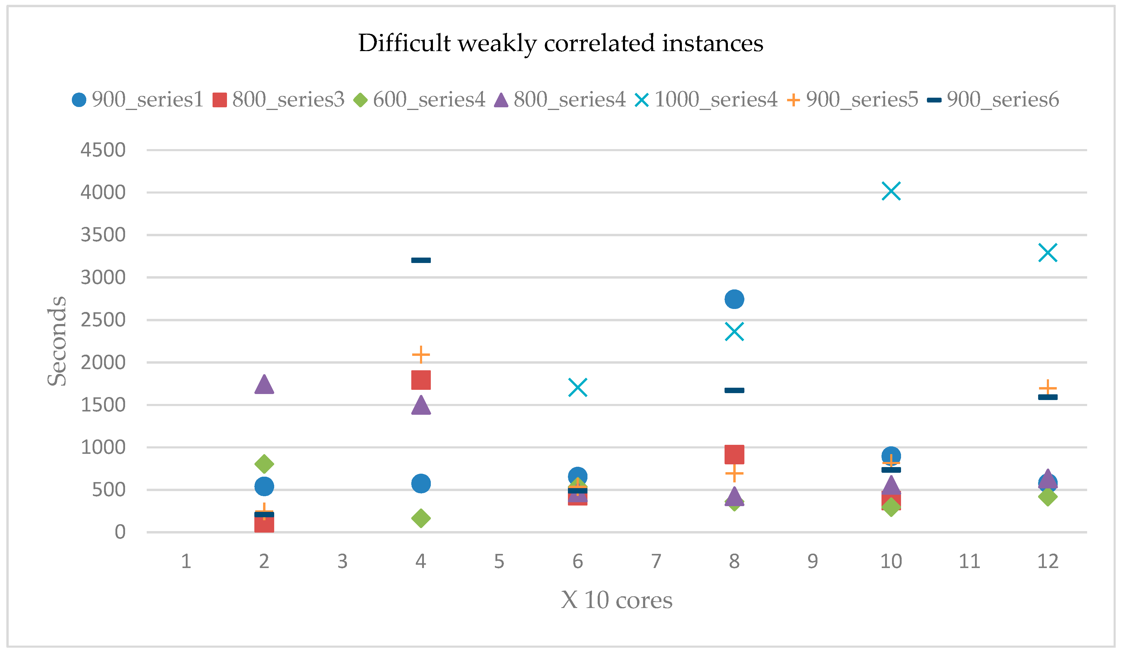
The application of the multi-BB algorithm for the problems of weakly correlated instances without sequential solutions was the same as in the previous problem. The results are shown in

Table 9. Difficult problems of weakly correlated instances (s).

Cores	900 Series 1	800 Series 3	600 Series 4	800 Serie 4	1000 Series 4	900 Series 5	900 Series 6
20	541.146778	113.254955	805.19268	1747.37338	---------	247.920172	207.720432
40	575.536042	1794.82854	166.197532	1502.92257	---------	2093.40998	3200.67639
60	655.732152	431.479931	535.095924	471.045603	1708.20222	536.465767	488.187185
80	2744.39269	916.620007	361.507553	425.59499	2364.02109	695.022149	1670.71194
100	897.756751	374.327425	297.126635	558.170916	4019.2701	817.248092	733.272021
120	578.094729	----------	420.501619	634.75545	3293.75821	1696.82872	1590.29178

and Figure 8.

The results in Table 9 and Figure 8 show that as the number of processing units increased, the dispersion of the results was smaller. Except for series 4, all others tended to be less variable for 100 processing units, and the variability increased again with 120 processing units. This indicates that the element that decreased the computations may have been a greater number of processing units. The same held true for series 4 with 1000 elements: it was only possible to determine its solution with a larger number of processing units.

5. Conclusions

From the results obtained, the following conclusions could be made:

It is possible to make binary branch-and-bound trees by fixing and removing subset elements to build a parallel algorithm, which calculates the optimal solution of the 0–1 knapsack problem.

Consideration of the four factors that affect the implementation of parallel algorithms is important, because they guide the process of obtaining efficient parallel algorithms, such as the one presented in this work.

The multi-BB algorithm calculated the optimal solution of the weakly correlated instances that could not be solved with the sequential version, instances that required excessive memory usage. This indicates that despite the fact that a larger number of search spaces were generated, the algorithm calculated the optimal solution without using the full memory of any server in the cluster. This shows that the moment when the global optimal function is updated is the correct one, because it allows for the pruning of a large number of binary tree branches assigned in the cores.

The parallel efficiencies reached were around 75%, but in some cases, it was possible to achieve superlinear speedup.

The improvement that can be made to the algorithm is to calculate, in a more efficient way, the elements that are fixed in the solution process, which perhaps could be done through hybridization of the algorithm. This will be a future task, along with including parallel programming via GPUs, which will allow for shared memory to be used and which will considerably accelerate communication between the procedures generated by the algorithm.

References

1. Bretthauer, K.M.; Shetty, B. The nonlinear knapsack problem-algorithms and applications. Eur. J. Oper. Res. 2002, 138, 459–472. [Google Scholar] [CrossRef]
2. Pisinger, D. Where are the hard knapsack problems? Comput. Oper. Res. 2005, 32, 2271–2284. [Google Scholar] [CrossRef]
3. Lv, J.; Wang, X.; Huang, M.; Cheng, H.; Li, F. Solving 0-1 knapsack problem by greedy degree and expectation efficiency. Appl. Soft Comput. 2016, 41, 94–103. [Google Scholar] [CrossRef] [Green Version]
4. Crainic, T.; Cun, B.; Roucariol, C. Parallel Branch and Bound Algorithms. In Parallel Combinatiorial Optimization, 1st ed.; Talbi, E.-G., Ed.; John Wiley & Sons: New York, NY, USA, 2006; pp. 1–28. [Google Scholar]
5. Gendron, B.; Crainic, T. Parallel Branch and Bound Algorithms: Survey and Synthesis. Oper. Res. 1994, 42, 1042–1066. [Google Scholar] [CrossRef]
6. Gmys, J.; Mezmaz, M.; Melab, N.; Tuyttens, D. IVM-based parallel branch-and-bound using hierarchical work stealing on multi-GPU systems. Concurr. Comput. Pract. Exp. 2017, 29, e4019. [Google Scholar] [CrossRef] [Green Version]
7. Shen, J.; Shigeoka, K.; Ino, F.; Hagihara, K. GPU-based branch-and-bound method to solve large 0-1 knapsack problems with data-centric strategies. Concurr. Comput. Pract. Exper. 2019, 31, e4954. [Google Scholar] [CrossRef]
8. Volosshinov, V.; Smirnos, S.; Sukhoroslov, O. Implementation and Use of Coarse-grained Parallel Branch and Bound in Everest Distributed Environment. Procedia Comput. Sci. 2017, 108, 1532–1541. [Google Scholar] [CrossRef]
9. Quan, Z.; Wu, L. Design and evaluation of a parallel neighbor algorithm for the disjunctively constrained knapsack problem. Concurr. Comput. Pract. Exp. 2017, 29, e3848. [Google Scholar] [CrossRef]
10. Vu, T.; Derbel, B. Parallel Branch-and-Bound in multi-core multi-CPU multi-GPU heterogeneous environments. Future Gener. Comput. Syst. 2016, 56, 95–109. [Google Scholar] [CrossRef] [Green Version]
11. Quinn, M.J. Designing Efficient Algorithms for Parallel Computers; McGrawHill Education: New York, NY, USA, 1987. [Google Scholar]
12. Goldman, A.; Trystram, D. An Efficient Parallel Algorithm for Solving the Knapsack Problem on Hypercubes. J. Parallel Distrib. Comput. 2004, 64, 1213–1222. [Google Scholar] [CrossRef]
13. Trienekens, H.W.J.M.; de Bruin, A. Towards a Taxonomy of Parallel Branch and Bound Algorithms, Report EUR-CS-92-01; Erasmus University Rotterdam, Department of Computer Science: Rotterdam, The Netherlands, 1992. [Google Scholar]
14. Li, K.; Liu, J.; Wan, L.; Yin, S.; Li, K. A cost-optimal parallel algorithm for the 0-1 knapsack problem and its performance on multicore CPU and GPU implementations. Parallel Comput. 2015, 43, 27–42. [Google Scholar] [CrossRef]
15. Melab, N.; Gmys, J.; Mezmaz, M.; Tuyttens, D. Multi-core versus many-core computing for many-task Branch and Bound applied to big optimization problems. J. Future Gener. Comput. Syst. 2018, 82, 472–481. [Google Scholar] [CrossRef] [Green Version]
16. Ismail, M.; el-raoof, O.; El-Wahed, W. A parallel Branch and Bound Algorithm for Solving Large Scale Integer Programming Problems. Appl. Math. Inf. Sci. 2014, 8, 1691–1698. [Google Scholar] [CrossRef] [Green Version]
17. Mathews, G.B. En la partición de números. Actas Lond. Math. Soc. 1897, 1, 486–490. [Google Scholar]
18. Dantzig, G.B. Discrete-Variable Extremum Problems. Oper. Res. 1957, 5, 266–277. [Google Scholar] [CrossRef]
19. Garey, M.R.; Johnson, D.S. Computers and Intractability: A Guide to the Theory of NP-Completeness; W.H. Freeman: San Francisco, CA, USA, 1979. [Google Scholar]
20. Martello, S.; Pisinger, D.; Toth, P. New trends in exact algorithms for the 0-1 knapsack problem, European. J. Oper. Res. 2000, 123, 325–332. [Google Scholar] [CrossRef]
21. Zavala-Díaz, J.C.; Ruis-Vanoye, J.A.; Díaz-Parra, O.; Hernández-Aguilar, J.A. A solution to the Strongly Correlated 0-1 Knapsack Problem by Binary Branch and Bound Algorithm. In Proceedings of the Fifth International Joint Conference on Computational Science and Optimization (CSO 2012), Harbin, China, 23–26 June 2012; pp. 237–241. [Google Scholar]
22. Zavala-Díaz, J.C.Y.; Khachaturov, V. Integer Programming, the Tree of Cubes Method, its Parallel Algorithm and Applications, Contexts in the Investigation of the Social and Administrative Sciences; Universidad Autónoma de Morelos: Cuernavaca, Mexico, 2006; pp. 77–102. [Google Scholar]
23. Aparicio, G.; Salmerón, J.M.G.; Casado, L.G.; Asenjo, R.; Hendrix, E.M.T. Parallel algorithms for computing the smallest binary tree size in unit simplex refinement. J. Parallel Distrib. Comput. 2018, 112, 166–178. [Google Scholar] [CrossRef]
24. Zavala-Díaz, J.C. Optimización con Cómputo Paralelo in Teoría y Aplicaciones; Zavala-Díaz, J.C., Ed.; AM editores-UAEM: Mexico City, Mexico, 2013. [Google Scholar]
25. Cormen, T.; Lerserson, C. Rivest Introduction to Algorithms; McGraw-Hill: New York, NY, USA, 2000. [Google Scholar]
26. Zhou, Y.; Chen, X.; Zhou, G. An improved monkey algorithm for a 0-1 knapsack problem. Appl. Soft Comput. 2016, 38, 817–830. [Google Scholar] [CrossRef] [Green Version]
27. Pospichal, P.; Schwarz, J.; Jaros, J.Y. Parallel genetic algorithm solving 0/1 knapsack problem running on the GPU. In Proceedings of the 16th International conference on soft computing, MENDEL 2010, Brno, Czech Republic, 23–25 June 2010; pp. 64–70. [Google Scholar]
28. Rizk-Allah, R.M.; Hassanien, A.E. New binary bat algorithm for solving 0-1 knapsack problem. Complex Intell. Syst. 2018, 4, 31–53. [Google Scholar] [CrossRef] [Green Version]
29. Archibald, B.; Maier, P.; McCreesh, C.; Stewart, R.; Trinder, P. Replicable parallel branch and bound search. J. Parallel Distrib. Comput. 2018, 113, 92–114. [Google Scholar] [CrossRef]
Figure 1. Search space P(m) of the set I = { 1 , 2 , 3 , 4 , 5 } [24].
Applsci 09 05368 g001
Figure 2. Binary tree of search spaces [24].
Applsci 09 05368 g002
Figure 3. Multi-BB (branch-and-bound) tree scheme.
Applsci 09 05368 g003
Figure 4. Flowchart of the parallel multi-BB algorithm.
Applsci 09 05368 g004
Figure 5. Uncorrelated instance runtime.
Applsci 09 05368 g005
Figure 6. Runtime of the weakly correlated instance.
Applsci 09 05368 g006
Figure 7. Workload of the 20 processing units for the problem in Figure 7.
Applsci 09 05368 g007
Figure 8. Difficult problems of a weakly correlated instance.
Applsci 09 05368 g008