Analysis of Elastic Nonlinearity Using Continuous Waves: Validation and Applications

Abstract

The nonlinear elastic response of consolidated granular or damaged materials is the result of the combination of nonlinear attenuation and velocity, coupled with hysteresis, which is linked to non equilibrium effects (often termed conditioning). Thus, a preliminary step towards the comprehension of the physical mechanisms responsible of the nonlinear elastic behaviours consists in quantifying and separating the various contributions. To this purpose, an approach based on a semi-analytical treatment of signals resulting from a monochromatic continuous wave excitation can be successfully implemented. Its validation is discussed here, applying the proposed approach to the analysis of numerical data obtained by using a finite difference spring model code. The accuracy, sensibility and robustness of the protocol are verified in different nonlinear conditions.

1. Introduction

Materials with a very different microstructure, including consolidated [1,2,3,4,5] and unconsolidated [6] granular media or damaged composites and metallic materials [7,8,9,10,11], share a very similar elastic behaviour, in which hysteresis plays a crucial role. Their nonlinear response to an ultrasonic excitation is governed by a combination of effects due to velocity dependence on strain and attenuation nonlinearity [12,13,14,15]. Furthermore, even more important are effects due to conditioning, relaxation and memory [16,17], i.e., the dependence of velocity and attenuation on time and maximum strain (history).

Qualitatively, the nonlinear behaviour of such materials looks very similar. On the contrary, their microstructure, which should suggest the physical mechanisms responsible of their elastic behaviour, is very different. Consolidated granular materials feature grain contacts, which may give rise to sliding [18] and/or static friction [19], together with adhesion mechanisms linked to the nonlinear behaviour due to the presence of water at the interfaces between microcracks faces [20,21]. On the other hand, in damaged composites, open or partially open cracks, responsible for clapping [22,23] or dislocations [24], are more likely to be the cause of the observed nonlinearities. Furthermore, the nonlinear elastic response increases dramatically in damaged materials. Again, the behaviour remains qualitatively the same, but the effects of the damaging processes, e.g., in consolidated granular media, could be very different: formation of open cracks for mechanical or thermal damaging [2,25,26,27], chemical reactions with expansive compounds in carbonation, corrosion or salt reactions [28,29,30], or even healing of cracks in some cases [31,32].

Consequently, it is hard to think of a single physical mechanism responsible for the elastic nonlinearity observed and, thus, it could be important to highlight differences in nonlinear materials with different microstructures, either intrinsic or damaged induced [33,34,35]. Nevertheless, to achieve this purpose, a finer analysis is necessary, which requires developing novel experimental approaches beyond those existing in the literature, i.e., harmonics and sidebands analysis [36,37], determination of the resonance frequency shift [25,38], quantification of the loss of proportionality [39,40], analysis of subharmonics [41] and others [42,43].

The development of a method which could cope with experimental and physical constraints is required, remaining at the same time able to separate nonlinearity due to damping from that due to elastic modulus [44,45]. In this regard, a method has been recently proposed [45], which makes use of a semianalytical analysis of experimental data obtained with a monochromatic continuous waves (cw) excitation in one dimensional samples.

The novelty of this contribution is manifold. Indeed, the aim of the present work is: (i) to confirm the correctness of the proposed method over a wide range of nonlinearity conditions (validation); (ii) to quantify the sensibility of the approach (quantification); and (iii) to establish the limits of its applicability (optimisation and robustness).

In the next section, we first present the approach to measure velocity and attenuation coefficient as a function of amplitude, by using a monochromatic continuous wave excitation. The approach is validated by analysing its efficiency in the treatment of synthetic data obtained using a numerical approach [46], also discussed in Section 2. Validation of the efficiency in separating nonlinearities, due to modulus or damping, is presented in Section 3. The validity of the approximations, needed to comply with experimental constraints when applying this approach, is discussed in Section 4. Finally, experimental results are shown in Section 5 to prove the suitability of the method to discriminate between different nonlinearities in different media.

2. Semianalytical Approach for the Determination of Modulus and Damping

2.1. The Method: Modulus and Damping Nonlinearities Evaluation (MoDaNE)

The MoDaNE approach described in the following aims to allow separating velocity and attenuation nonlinearities. It takes advantage of an exact analytical solution of the 1D problem of monochromatic waves propagation in elastic bars. Of course, an analogous approach extended to 2D or 3D general cases would be more complete and also allow addressing issues which are not specific to a 1D problem, such as those connected to directionality of nonlinear effects [47]. Nevertheless, a 1D solution maintains its relevance, since a large number of samples and configurations used in laboratory experiments can be usually considered 1D (e.g., cylinders, rods or prisms) and also 1D geometries are often of interest in applications.

2.1.1. One-Dimensional Solution

The equation of motion for a 1D linear elastic medium, during the propagation of an elastic wave, can be easily written as:

$$\begin{array}{c}\hfill \rho \frac{{\partial }^{2}u}{\partial t^2}+\lambda \frac{\partial u}{\partial t}=S\frac{{\partial }^{2}u}{\partial x^2}\end{array}$$

(1)

where $u(x,t)$ denotes the longitudinal displacement, $\rho$ is the density, $\lambda$ is the damping parameter and S is the elastic modulus. In the case of an infinite medium (or semi-infinite with a monochromatic forcing $F\left(t\right)$ in $x=0$), the solution is a monochromatic wave:

$$\begin{array}{c}\hfill u(x,t)=U_0{e}^{-\alpha x}{e}^{j(\omega (t-t_0)-kx)}\end{array}$$

(2)

with phase ${\varphi }_0=-\omega t_0$ and amplitude $U_0$ at $x=0$ and $t=0$. The dispersion relation provides the phase velocity $c=\omega /k$ and the Q-factor is derived from $Q=\omega /\alpha c$.

There is a strong relation between the wave number k, the attenuation coefficient $\alpha$, the elastic modulus S and the damping parameter $\lambda$. Indeed, substituting the solution (Equation (2)) into the wave equation (Equation (1)), one can derive the following expressions:

$$\begin{array}{c}\hfill S=\frac{\rho {\omega }^2}{(k^2-{\alpha }^2)}\end{array}$$

(3)

$$\begin{array}{c}\hfill \lambda =-\frac{2\alpha kS}{\omega }\end{array}$$

(4)

The solution remains valid also in the presence of different attenuation mechanisms described by different terms in Equation (1), but a different relation between the damping parameter $\lambda$ and the attenuation coefficient $\alpha$ is expected in this case. Furthermore, as discussed below, the equation and solutions remain approximately valid also in the case of weakly nonlinear media, in which only small distortions of the signal are detected. In this case, the effective modulus and damping play the same role as S and $\lambda$, averaging over a period and over the propagation path.

Taking into account a finite medium of length L with free-free boundary conditions, the analytical solution in $x=L$ can be derived considering the solution as the superposition of multiple reflections:

$$\begin{array}{c}\hfill u^{+}(x,t)=\sum _{n=1}^{\infty }{U}_0{e}^{j(\omega t-k(2(n-1)L+x))+{\varphi }_0}{e}^{-\alpha \left(2\right(n-1)L+x)}\\ \hfill u^{-}(x,t)=\sum _{n=1}^{\infty }{U}_0{e}^{j(\omega t-k(2nL-x))+{\varphi }_0}{e}^{-\alpha (2nL-x)}\\ \hfill u(x,t)=u^{+}(x,t)+u^{-}(x,t)\end{array}$$

(5)

The solution in ($x=L$) is still a sinusoidal monochromatic wave, but with different amplitude A and phase $\varphi$:

$$\begin{array}{c}\hfill u(L,t)=A{e}^{j(\omega (t-t_0)+\varphi )}\\ \hfill =A{e}^{j(\omega t+\Phi )}\end{array}$$

(6)

where their analytical expressions are

$$\begin{array}{c}\hfill A=\frac{U_0}{\sqrt{{cosh}^2\left(\alpha L\right)-{cos}^2\left(kL\right)}}\end{array}$$

(7)

$$\begin{array}{c}\hfill \varphi =-arctan\frac{tan\left(kL\right)}{tanh\left(\alpha L\right)}\end{array}$$

(8)

It is useful to recall that $U_0$ and ${\varphi }_0$ are the amplitude and phase of the solution at $x=0$ (see Equation (2)).

2.1.2. Inversion: Dispersion Relation and Attenuation Coefficient

The analytical derivation of Equations (7) and (8) can be exploited to extract velocity c and attenuation coefficient $\alpha$ from experimental data. To do this, let us consider to excite a 1D sample, at $x=0$, with a sinusoidal wave of frequency $\omega$. The output signal at $x=L$ is recorded and its amplitude A and phase $\Phi =\varphi +{\varphi }_0$ (with ${\varphi }_0=-\omega t_0$) can be derived by fitting experimental data with a cosine function. Furthermore, by using a suitable calibration of the experiment, $U_0$ and ${\varphi }_0=-\omega t_0$ can be also derived. Hence, the phase $\varphi =\Phi -{\varphi }_0$ can be measured.

Inverting Equations (7) and (8), the analytical expressions of the physical quantities velocity c and attenuation coefficient $\alpha$ can be derived:

$$\begin{array}{c}\hfill c=\omega /k=\frac{\omega }{\frac{1}{L}\left(\pi n\pm atan\sqrt{\frac{z}{2{cos}^2\left(\varphi \right)}}\right)}\end{array}$$

(9)

$$\begin{array}{c}\hfill \alpha =\frac{1}{L}atanh\sqrt{\frac{z}{2{sin}^2\left(\varphi \right)}}\end{array}$$

(10)

where the sign is positive if $\varphi +{\varphi }_0>0$, n is the order of the closest mode to $\omega$ and

$$z=-{(A/U_0)}^2-cos\left(2\varphi \right)+\sqrt{1+{(A/U_0)}^4+2cos\left(2\varphi \right){(A/U_0)}^2}$$

(11)

2.2. Numerical Solutions

2.2.1. Numerical Approach

In order to investigate the influence of the physical and experimental constraints on the analysis, the discussed approach was applied to synthetic data. In this way, the efficiency and robustness of the proposed procedure may be quantified by comparing the results of the analysis with the known theoretically expected values, i.e. the input parameters of the simulation.

Numerical data were obtained simulating, with a finite difference spring-model approach [48], the propagation of elastic waves in classical nonlinear media, described by the classical wave equation Equation (1). Details about the numerical solutions could be found in Ref. [46,48]. For the sake of simplicity, the nonlinear contributions due to hysteresis were not considered.

The following expansions of the linear parameters as a function of the strain tensor were considered:

$$\begin{array}{c}\hfill S=S_0\left(1+{\delta }_S{ϵ}^2+{\gamma }_S{ϵ}^4\right)\\ \hfill \lambda ={\lambda }_0\left(1+{\delta }_{\lambda }{ϵ}^2+{\gamma }_{\lambda }{ϵ}^4\right)\end{array}$$

(12)

where $S_0$ and ${\lambda }_0$ are the linear (at low amplitude of excitation) values of modulus and damping, respectively. $ϵ=\partial u/\partial x$ is the strain and $u(x,t)$ is the displacement (dependent on time t and space x). For the simulations, a 1D sample 10 cm long, with $S_0=72$ GPa, ${\lambda }_0=6.48$${10}^2$ s ${}^{-1}$ and density $\rho =2700$ kg/m ${}^3$ was considered, unless otherwise specified. The values of the nonlinear parameters ${\delta }_S$, ${\gamma }_S$ and ${\delta }_{\lambda }$ were changed in the different simulations and are reported in the table of Figure 1. Notice that ${\gamma }_{\lambda }$ was set equal to zero for all simulations. Indeed, quartic nonlinear terms are usually negligible in real materials for both modulus and damping. Here, a non-negligible quartic nonlinearity on the elastic modulus was considered only for the sake of demonstrating that the MoDaNE approach is capable of capturing different power law behaviours in the velocity/attenuation vs. strain dependence.

2.2.2. Estimation of Nonlinear Parameters on Velocity and Attenuation

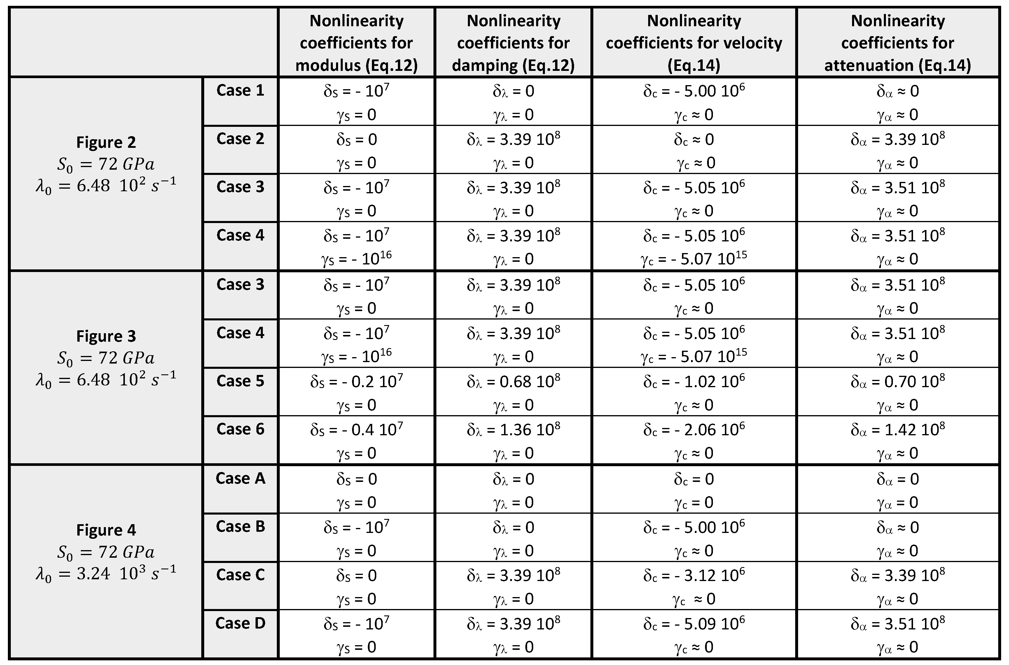
From Equations (3) and (4), it is possible to derive the expressions which evidence how nonlinearities on modulus and damping may determine nonlinearities on velocity and attenuation:

$$\begin{array}{c}\hfill c=\sqrt{\frac{S}{\rho }\frac{2}{(1+{\lambda }^2/\left({\rho }^2{\omega }^2\right))}}\\ \hfill \alpha =\frac{c\lambda }{2S}\end{array}$$

(13)

It follows that nonlinearity on velocity c is due to both nonlinearities on modulus S and damping $\lambda$, and similarly for what concerns nonlinearity on attenuation $\alpha$.

Normally, in the literature, it is assumed that nonlinearities on c and $\alpha$ are decoupled, in the sense that, assuming small $\lambda$ and small nonlinearity on S, we have:

$$\begin{array}{c}\hfill \frac{\Delta c}{c_0}=\frac{1}{2}\frac{\Delta S}{S_0}\\ \hfill \frac{\Delta \alpha }{{\alpha }_0}=\frac{\Delta \lambda }{{\lambda }_0}\end{array}$$

(14)

However, as we shown here, this is not always the case, since Equation (13) provides a more complex relation. Substituting the Taylor expansion for S and $\lambda$, in principle the nonlinear dependence of c and $\alpha$ could be derived with a Taylor expansion for small strains:

$$\begin{array}{c}\hfill c=c_0\left(1+{\delta }_c{ϵ}^2+{\gamma }_c{ϵ}^4\right)\\ \hfill \alpha ={\alpha }_0\left(1+{\delta }_{\alpha }{ϵ}^2+{\gamma }_{\alpha }{ϵ}^4\right)\end{array}$$

(15)

The analytical solution is very cumbersome and it is not reported here.

A simpler procedure to estimate the coupling between modulus/damping and velocity/attenuation nonlinearities can be adopted. For given values of modulus/damping nonlinear parameters, c and $\alpha$ can be derived using Equation (13) and plotted vs. strain. The resulting curves are fit with a polynomial function to derive numerically the coefficients of Equation (15). An example of derivation is shown in Figure 2.

Results of the calculation for the various cases analysed in the following are reported in the last two columns of the table in Figure 1. We recall that in the cases considered in this paper we always have ${\gamma }_{\alpha }\approx 0$, since the input nonlinear parameter ${\gamma }_{\lambda }$ was always set equal to zero. Results indicate that neglecting, as often done, the effects of damping nonlinearity on velocity nonlinearity is not always correct, while even more critical is neglecting modulus nonlinearity effects on attenuation coefficient nonlinearity. Indeed:

• For Cases 1 and 2, ${\delta }_c=$$0.5$${\delta }_S$. In Case 3, the relationship between ${\delta }_c$ and ${\delta }_S$ given by Equation (14) is still approximately valid, being the effect of ${\delta }_{\lambda }$ on ${\delta }_c$ about 1% only.
• In all cases, the effect of modulus nonlinearity ${\delta }_S$ on attenuation nonlinearity ${\delta }_{\alpha }$ is more significant (more than 3% in Case 3). Therefore, the assumption $\Delta \lambda /{\lambda }_0=\Delta \alpha /{\alpha }_0$ is not accurate. The effect increases when increasing the modulus nonlinear parameter.
• In the case of materials with high damping, Cases C and D, a significant effect of damping nonlinearity ${\delta }_{\lambda }$ on velocity nonlinearity is found and $\Delta c/c_0\ne$$0.5$$\Delta S/S_0$.

2.2.3. Numerical Analysis

Several simulations were performed varying the input parameters describing the nonlinearity: ${\delta }_S,{\gamma }_S$ and ${\delta }_{\lambda }$. For each simulation, the excitation source (simulating a PZT transducer) was chosen as a monochromatic forcing applied in $x=0$:

$$F(0,t)=B_{i}cos\left(\omega t\right)$$

(16)

with varying amplitude $B_i$ and frequency $\omega$. Frequency was chosen close to the first linear resonance mode: $\omega =25.82$ kHz. The corresponding output signals $u_i\left(t\right)$ were recorded in $x=L$, as required by the proposed approach and as done in experiments (using a PZT receiving transducer or laser vibrometer). To simulate noise, a white noise $n_i\left(t\right)$ was added to the detected signals, with amplitude corresponding to 5% of the amplitude of the signal detected at the lowest amplitude of excitation ($u_1\left(t\right)$), corresponding to the order of magnitude of the signal-to-noise ratio usually observed in experiments.

The numerical results were treated using the Modulus and Damping Nonlinearities Evaluation method (MoDaNE), previously discussed in this section, in order to derive the dependence of attenuation and velocity on amplitude from the recorded signals. To validate the approach, our aim was:

• to verify the capability of the approach to separate nonlinearity in $\alpha$ and c, comparing Cases 1, 2 and 3;
• validate the possibility to reproduce qualitatively the expected functional dependences (quadratic or quartic plus quadratic) of c and $\alpha$ on strain: comparison of Cases 3 and 4;
• verify that the approach allows to detect the effects of S/$\lambda$ nonlinearities on c/$\alpha$ nonlinearities: Cases 3 and C; and
• verify that, at least in some circumstances as shown below, the approach allows quantifying correctly the nonlinear parameters ${\delta }_c,{\gamma }_c$ and ${\delta }_{\alpha }^{\prime }$: Cases 3, 5 and 6.

3. Validation

3.1. Feasibility of the Separation of Modulus and Damping Contributions

Understanding the functional dependence of c and $\alpha$ on strain is a first goal of the analysis of nonlinear elasticity in complex media, since it allows observing differences for different materials. As discussed above, nonlinearities in velocity are normally associated to modulus nonlinearities, while nonlinearities in attenuation coefficient are associated to damping nonlinearities.

However, as we have shown, some corrections must be considered and this could be important in particular cases, e.g., for strongly attenuative media. Here, we focus on validating the capability of the method to separate correctly the two kind of nonlinearities.

3.1.1. Low Linear Damping

When damping is low (high Q-factor materials), Equation (13) and table reported in Figure 1 suggest that the velocity dependence on amplitude is due only to the modulus nonlinearity (being the damping contribution to velocity very small). Furthermore, if damping nonlinearity is strong, contribution of modulus nonlinearity to the amplitude dependence of attenuation coefficient is slightly more significant but still almost negligible.

To validate our approach under these conditions, numerical simulations were performed for the four combinations of nonlinear parameters reported in Figure 1. More specifically, we consider here a quadratic nonlinearity for damping parameter (Case 1), quadratic nonlinearity for elastic modulus (Case 2), quadratic nonlinearity in both modulus and damping (Case 3) and quartic and quadratic nonlinearity in modulus and quadratic nonlinearity in damping (Case 4).

Results of the analysis of the data are reported in Figure 3, where the relative variations of velocity and attenuation coefficient (respect to their corresponding linear values) are reported vs. amplitude A. The analysis of the data demonstrates that:

• The method allows separation of modulus and damping contributions. Indeed, in Cases 1 and 2, in which only one physical parameter is nonlinear (either S or $\lambda$), only the corresponding measurable quantity (either c or $\alpha$) manifests nonlinearity.
• The method allows determining accurately the functional dependence on A of velocity and attenuation coefficient relative variations. Curves were fitted with a polynomial function in the form:

  $$y=q_1{A}^2+q_2{A}^4$$

  (17)

  While in Cases 1, 2 and 3 the fitting coefficient $q_2$ was negligible (for the velocity dependence on A), in Case 4 the coefficient plays a crucial role (more details in comments on Figure 4).
• In this analysis, there is no quantitative prediction of the nonlinear parameters. Indeed, numerical solutions were based on a dependence of velocity and attenuation on strain, and not on displacement amplitude. Hence, as expected, the fitting coefficients $q_1$ and $q_2$, both for the relative variations of velocity and attenuation, do not correspond to the nonlinear parameters used as input in the numerical code. A quantitative analysis, which is discussed in Section 3.2, is possible but it implies further considerations.

3.1.2. Estimation of the Relative Weight of Nonlinearities

As discussed in the previous subsection, the method was proven to be efficient in qualitatively identifying the functional dependence of c and $\alpha$ on strain. This is useful to support the development of physical models, aiming to describe nonlinearity. Furthermore, this approach in principle allows comparing nonlinearities in different media studied experimentally in the same conditions, with obvious implications for materials characterisation and particularly for quantitative non destructive testing.

To demonstrate the feasibility of such analysis, we demonstrate here the proportionality between the true nonlinear parameters (input of simulations) and the corresponding nonlinear coefficients of the fitting of Equation (17). To this purpose, velocity and attenuation coefficient variations vs. amplitude A are plotted, in log-log scale, in Figure 4 for different cases.

Results reported in Figure 4 show that:

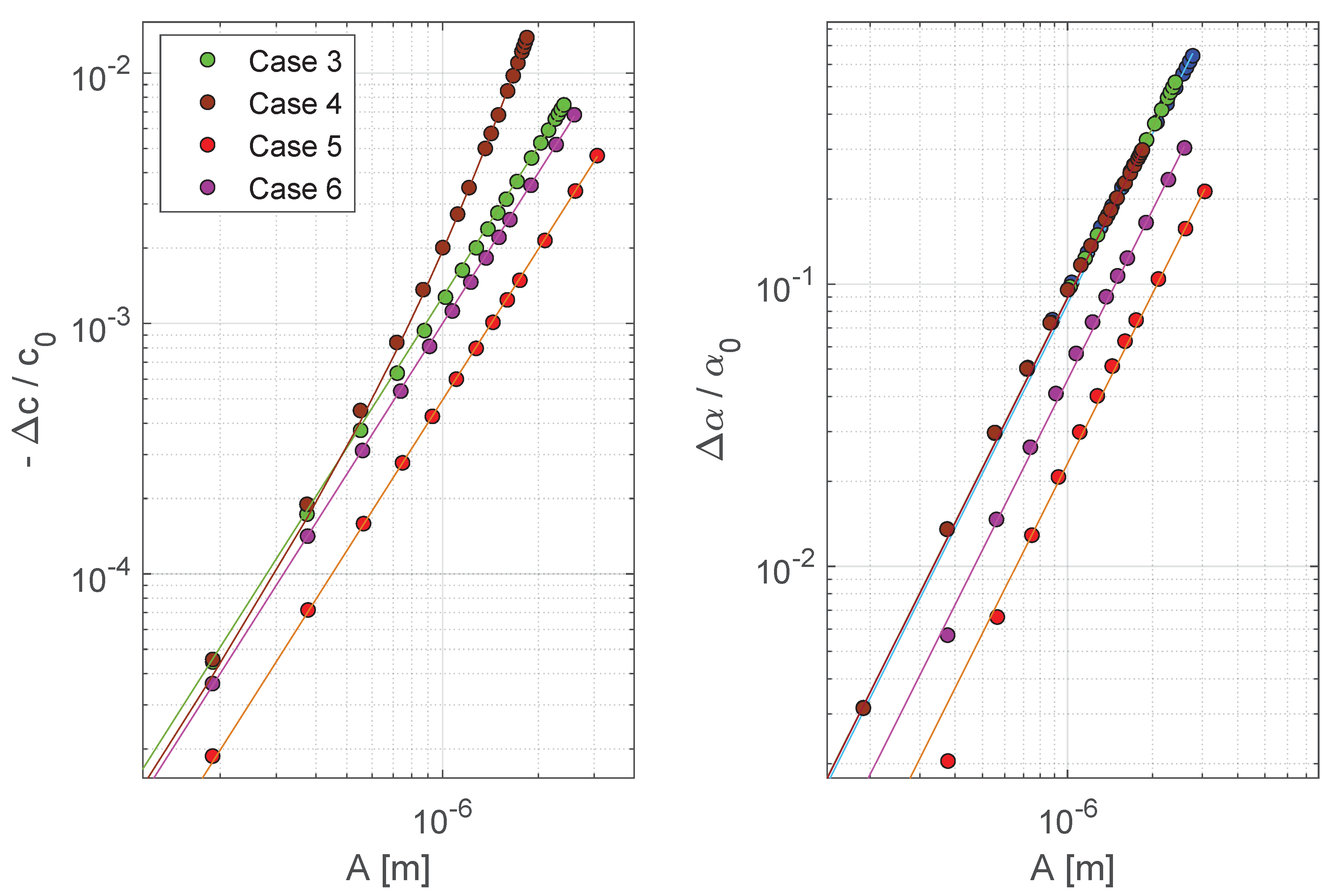
• The curves are straight lines with slope 2 (we recall that the slope in log-log scale of a power law function corresponds to the power law exponent), except for velocity in Case 4. Indeed, in this case, the modulus dependence on strain is not a power law (see also Equation (12)). It is important to observe that in this case the power law quadratic dependence of damping is still well reconstructed by the analysis.
• Cases 5 and 6 differ from Case 3 only because the nonlinear parameters are scaled: ${\delta }_S\to k{\delta }_S$ and ${\delta }_{\lambda }\to k{\delta }_{\lambda }$. In both cases, the slope of the curves describing c and $\alpha$ vs. amplitude remains 2 (as expected). Furthermore, the vertical shift of the curves of a quantity $\Delta$ with respect to that of Case 3 preserves the proportionality with respect to the theoretical nonlinear coefficients. Indeed, results of the fit show that for each of the two cases $\Delta \approx 20lo{g}_{10}\left(k\right)$. Therefore, monitoring nonlinearity evolution as a function of time, in samples subjected to progressive damage, is feasible with the proposed approach.

3.1.3. High Linear Damping

As mentioned, Equation (3) suggests that nonlinearity of the damping parameter $\lambda$ has influence on nonlinearity in velocity c. Normally, the damping contribution to velocity is negligible, but this is no longer true when ${\lambda }_0$ is large. Here, the goal is to prove that the approach proposed in this paper can also deal with such extreme cases.

To this purpose, we compare the results of Figure 3 (obtained when linear damping is low: ${\lambda }_0=6.48\times {10}^2$ ${\mathrm{s}}^{-1}$), with those obtained in the case of high linear damping (${\lambda }_0=3.24\times {10}^3$ $s^{-1}$), reported in Figure 5. Details on nonlinear parameters used in simulations for all the cases, are reported in the table of Figure 1. Note that in Case B only the modulus was chosen to be nonlinear (${\delta }_S\ne 0,{\delta }_{\lambda }=0$) and its nonlinearity is supposed to have a small effect on attenuation nonlinearity; in Case C only the damping was chosen to be nonlinear (${\delta }_S=0,{\delta }_{\lambda }\ne 0$) and its nonlinearity is supposed to have a small but identifiable effect on velocity nonlinearity.

Hence, it is possible to note that:

• Case A: As expected, in the linear case, there are no variations on both velocity and attenuation coefficient.
• Cases B and D: In both cases, nonlinearity in c (Case B) or both in c and $\alpha$ (Case D) are observed, as expected. For attenuation coefficients with respect to the expected behaviour for the two cases, this is not the case for the estimated velocity nonlinearity, even though the nonlinear modulus parameters are the same for the two cases. The slight difference (appreciable for high strain levels) is due to the small damping contribution to velocity nonlinearity when damping is strong.
• Case C: In this case, the effects of damping nonlinearity on velocity are more easily appreciated. In fact, the imposed quadratic nonlinearity on damping induces nonlinearity on attenuation coefficient as well as on velocity (green circles).

3.1.4. Hysteresis

Finally, the MoDaNE approach in presence of hysteretic nonlinearity was also validated. In this case, as a consequence of memory effects, the material parameters at a given amplitude of excitation depend not only on the actual nonlinearity, but also on the previous stress history. It follows that a hysteretic loop is observed when considering the dependence of velocity (and attenuation) on strain applying a protocol with increasing and then decreasing amplitudes of excitation [15].

To prove the capability of the MoDaNE approach in separating velocity and attenuation nonlinearities also in the presence of hysteresis, numerical simulations were performed using a phenomenological model. The model, described in [49] and validated in [46,50], is based on a Preisach–Maiergoytz approach in which hysteresis in modulus and damping are linked together. Results of the analysis of the numerical data are reported in Figure 6 and allow observing that the MoDaNE approach is sensitive to memory effects.

3.2. Quantitative Behaviour

As discussed in Section 3.1, the parameters derived by fitting the curves of the relative variations of velocity and attenuation vs. amplitude do not correspond to those theoretically expected. This is not surprising, since S and $\lambda$ (and hence c and $\alpha$) are defined as a function of strain. In addition, detected signals (both numerically and experimentally obtained) are resulting from waves travelling in space and time and are analysed using a long time window (a few cycles of the signals). Hence, the nonlinear signature contained in the signal is the result of averaging nonlinearities over space and time. Equivalently, it is feasible asserting that for each amplitude A, the signals are influenced by an averaged strain.

Thus, a comparison of the theoretical values of the nonlinear parameters (${\delta }_c^{th},{\gamma }_c^{th}$ and ${\delta }_{\alpha }^{th}$, i.e., the input parameters of the simulations derived in the table of Figure 1) and the coefficients of the polynomial fitting of the curves obtained from the analysis of numerical data of curves reported in Figure 3 (${\delta }_c^{fit},{\gamma }_c^{fit}$ and ${\delta }_{\alpha }^{fit}$), must be carefully performed. Indeed, we could expect that:

$$\begin{array}{c}\hfill c_{th}=c_0\left(1+{\delta }_c^{th}{ϵ}^2+{\gamma }_c^{th}{ϵ}^4\right)\\ \hfill c_{measured}=c_0\left(1+{\delta }_c^{fit}<{ϵ}^2>+{\gamma }_c^{fit}<{ϵ}^4>\right)\end{array}$$

(18)

and similarly for $\alpha$. In Equation (18), the symbols “$<>$” represent the average over space (between 0 and the sample length L) and time (between 0 and one period T).

Furthermore, as shown in Appendix C, averaged quadratic and quartic strains are proportional to the amplitude A of the displacement at $x=L$ (hence, the preservation of proportionality discussed before). Therefore,

$$\begin{array}{c}\hfill <{ϵ}^2(x,t)>=K_1^2{A}^2\\ \hfill <{ϵ}^4(x,t)>=K_2^4{A}^4\end{array}$$

(19)

where $K_1\ne K_2$ and both could be analytically calculated and depend on $S_0$, ${\lambda }_0$ (connected to $c_0$ and ${\alpha }_0$ as discussed previously) and L, as shown in Appendix C. It follows that

$$\begin{array}{c}\hfill c_{measured}=c_0\left(1+{\delta }_c^{fit}{K}_1^2{A}^2+{\gamma }_c^{fit}{K}_2^4{A}^4\right)\\ \hfill {\alpha }_{measured}={\alpha }_0\left(1+{\delta }_{\alpha }^{fit}{K}_1^2{A}^2\right)\end{array}$$

(20)

Thus, when fitting the measured curves (e.g., those in Figure 3) with a polynomial function,

$$\begin{array}{c}\hfill \Delta c_{measured}/c_0=q_1{A}^2+q_2{A}^4\\ \hfill \Delta {\alpha }_{measured}/{\alpha }_0=r_1{A}^2\\ \hfill \end{array}$$

(21)

we obtain the estimated nonlinear parameters as:

$$\begin{array}{c}\hfill {\delta }_c^{fit}=q_1/K_1^2\\ \hfill {\gamma }_c^{fit}=q_2/K_2^2\\ \hfill {\delta }_{\alpha }^{fit}=r_1/K_1^2\end{array}$$

(22)

Calculations were performed and results are shown in

Table 1. Theoretical nonlinear parameters (input of the simulations) and derived nonlinear parameters obtained as described in the main text: Equation (22). We analysed the data shown in Figure 3.

NL		Case 1	Case 2	Case 3	Case 4
${\delta }_c$	${\delta }_c^{th}$	$-5.00$ × ${10}^6$	0	$-5.05$ × ${10}^6$	$-5.06$ × ${10}^6$
	${\delta }_c^{fit}$	$-5.01$ × ${10}^6$	$\approx 0$	$-5.07$ × ${10}^6$	$-4.23$ × ${10}^6$
${\gamma }_c$	${\gamma }_c^{th}$	0	0	0	$-5.07$ × ${10}^{15}$
	${\gamma }_c^{fit}$	$\approx 0$	$\approx 0$	$\approx 0$	$-6.31$ × ${10}^{15}$
${\delta }_{\alpha }$	${\delta }_{\alpha }^{th}$	0	$3.39$ × ${10}^8$	$3.51$ × ${10}^8$	$3.51$ × ${10}^8$
	${\delta }_{\alpha }^{fit}$	$\approx 0$	$3.38$ × ${10}^8$	$3.56$ × ${10}^8$	$3.54$ × ${10}^8$

for the data reported in Figure 3. We obtain an excellent agreement between measured nonlinear parameters with those theoretically expected in Cases 1, 2 and 3. The efficiency of the approach in detecting accurately effects of nonlinearities in modulus/damping on nonlinearities in velocity/attenuation (Case 3) is remarkable.

The estimation of nonlinear parameters of velocity is poorer when the dependence of the nonlinear parameter is a combination of two power laws (quadratic and quartic). We have a reasonable (at least as far as the order of magnitude is concerned) estimation of both quadratic and quartic nonlinear parameters, but the error increases to about 15–20%. This is probably due to the fact that the hypothesis of Equation (18) is no longer valid. The estimated parameters for attenuation are still well predicted.

In conclusion, quantification of the nonlinear parameters is thus satisfactory, with small errors when nonlinearity (either in modulus or damping) is a power law function of strain (Cases 1–3). In more complex situations, errors could be larger and perhaps alternative approaches should be identified (work in progress).

4. Efficiency and Robustness of the Approach

Besides having verified the efficiency of the approach, the robustness of the procedure is studied here, also in view of a possible optimisation. In this section, simulations were performed considering the values of the nonlinear parameters used in simulations for Case 3 in the table of Figure 1, i.e., quadratic nonlinearity for both S and $\lambda$.

4.1. Frequency Dependence

Robustness of the approach was tested by first verifying that results are independent from the choice of the testing frequency. To this purpose, quadratic nonlinearity on both S and $\lambda$ were considered and the procedure was applied varying the frequency of the excitation around the first resonance mode. The linear resonance frequency was at $\omega ={\omega }_r=25.82$ kHz. Plots in Figure 7 report velocity and attenuation variations as a function of the averaged quadratic strain, as defined in Equation (19).

The results show that both amplitudes and phases vary with different functional dependences on the averaged quadratic strain. This is expected as a result of the shift of the resonance frequency which could give an apparent increase in amplitude, even though damping is increasing. On the contrary, variations of velocity and attenuation coefficient, calculated using the proposed method, result to be frequency independent.

4.2. Dependence on Calibration Errors

One of the major sources of possible errors in the proposed approach is related to the numerical calibration procedure. In Figure 8, the effects of errors on the calibration parameters $U_0$ and ${\varphi }_0$ (indicated with $w_{U_0}$ and $w_{{\varphi }_0}$, respectively) in the estimation of quadratic nonlinear parameters are shown. Here, the relative errors in velocity and attenuation coefficient are plotted, obtained from the analysis of the simulation data with respect to those theoretically expected, in the case of quadratic nonlinearities imposed both on modulus and damping.

The error in the quantitative determination of the nonlinear parameters increases roughly proportionally to the errors in the calibration procedure. It is interesting to note that errors in the calibration amplitude $U_0$ have negligible influence on the attenuation coefficient (Figure 8d). On the contrary the estimation of the attenuation nonlinear parameter ${\delta }_{\alpha }$ is extremely sensitive to errors in the calibration phase ${\varphi }_0$ (Figure 8b). Instead, the influence of errors on $U_0$ and ${\varphi }_0$ in the estimation of the velocity nonlinear quadratic parameter ${\delta }_c$ is of the same order of magnitude.

It is worth pointing out here that in experiments calibration of the phase is always very accurate, thus errors induced by calibration could be confined to a range of few per cent. Concluding this section, it is also notable to highlight that errors in the calibration do not affect at all the determination of the functional dependence of velocity and attenuation coefficient on strain.

4.3. Dependence on Signal Distortions

The proposed procedure is based on fitting experimental data with a sinusoidal function. The presence of nonlinearity induces distortions of the signals from the pure cosine wave behavior, e.g., due to the appearance of higher order harmonics. In general, being nonlinearity weak, distortions are negligible and the approach is expected to work well.

However, for strong nonlinearities (or large amplitudes), the proposed procedure might no longer be correct. The problem was analysed and results are presented in Figure 9. Simulations were carried out varying the nonlinear parameter ${\delta }_S$ (keeping fixed the nonlinear parameter on damping ${\delta }_{\lambda }$) and the relative error in the estimate of the nonlinear parameters of velocity ${\delta }_c$ and attenuation ${\delta }_{\alpha }$ are calculated as a function of the distortions of the signal. The latter are estimated as the ratio of generated third harmonic amplitude over fundamental harmonic amplitude.

As expected, increasing the nonlinear parameters corresponds to increasing distortions of the signal and the estimation obtained from our method becomes poorer and poorer. However, in particular for the velocity nonlinearity (Figure 9, left), the accuracy remains excellent up to a few per cent of distortion, which is high if compared to nonlinearity observed in the cases of interest.

5. Experimental Validation

To show an actual implementation of MoDaNE approach and its ability to discriminate between different nonlinearities in different media, a few experimental results are presented in this section. The characteristics of the investigated samples are the following:

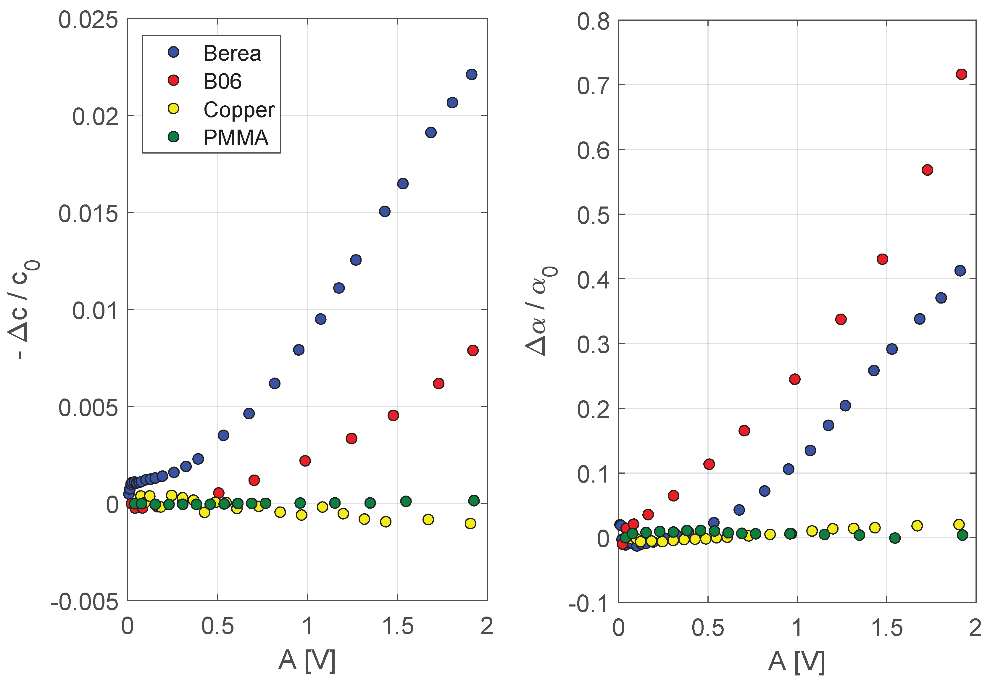
• The concrete sample (B06) was in the shape of a cylinder (4 cm diameter and 16 cm length), and was drilled from a casting prepared with 340 kg of cement (CEM II A-L 42.5 R), 957 kg of sand (0–5 mm), 846 kg of gravel (5–15 mm) and 200 kg of water (w/c ratio $\approx 0.59$).
• The Berea sandstone sample was a thin cylinder with a diameter of 1 cm and 15 cm long. The size of the grains in this sample is of the order of tens of micrometers.
• The two linear samples (PMMA and copper) were in the shape of cylinders (section of $2.25$ cm${}^2$ and length of $14.5$ cm). Both samples were intact.

The experiments were carried out as follows. A waveform generator (Tektronix AFG 3022B) generating monochromatic waves at increasing amplitudes is connected to a linear amplifier (CIPRIAN Model US-TXP-3, 200×). Two ultrasonic sensors with a diameter of 2.5 cm and a centre frequency at 55 kHz (MATEST C370-02) were connected one to the amplifier (source) and the other (receiver) to a digital oscilloscope (Lecroy 324A) for data acquisition. The signals, recorded in a short time window in standing wave conditions, are monochromatic waves and treated using the MoDaNE approach described before. Furthermore, the linearity of the system (including transducers and coupling media) was verified before starting the measurements.

In Figure 10, it is easy to observe that copper and PMMA behave linearly and no variation in c and $\alpha$ is present increasing the amplitude of excitation. Differently, the other two samples (consolidated granular media) exhibit high nonlinearity, both for relative variations of velocity and attenuation. However, some differences, most probably due to very different grain structures, can be appreciated: B06 shows a higher nonlinearity in the attenuation coefficient $\alpha$ with respect to Berea sandstone, while the situation is the opposite when the variation of velocity c is considered for the two samples.

6. Conclusions

We discuss here the efficiency, robustness and limitations of an approach recently proposed [45] and able to measure the nonlinearity in velocity and attenuation coefficient and separate their contributions. This method, based on a semi-analytical solution of the problem valid for quasi one-dimensional samples, is a faster and simpler alternative to standard approaches, such as nonlinear resonant ultrasound spectroscopy [51], nonlinear elastic wave spectroscopy [12] or Dynamic AcoustoElastic Testing [52].

The optimisation and definition of the limits of the MoDaNE approach are discussed by using the method to invert virtual data (resulting from numerical simulations). Different nonlinear cases were investigated and results show that the method allows measuring independently nonlinearity in velocity and attenuation coefficient and therefore to monitor their dependence on strain. The approach is extremely efficient in determining the coupling between modulus/damping nonlinearities and velocity/attenuation nonlinearities, which are normally neglected in other approaches. The robustness of the approach in determining the functional dependence of velocity and attenuation on strain has been demonstrated and the importance of a correct calibration has been quantified as well.

As far as quantification of nonlinear parameters is concerned, some approximations/hypothesis have to be added. Since ultrasonic measurements, in which multiple reflections are present, detect signals resulting from the superposition of waves travelling along different paths, the nonlinear signature is intrinsically averaged over time and space. In the case of pure power law nonlinearities, assuming measured velocities and attenuation to be dependent on averaged quadratic strains, the discussed method provides an excellent approach to quantify correctly the nonlinear parameters. In more complex situations, e.g., when the nonlinear dependence is not quadratic or when conditioning is present [53], other approaches must be developed.

The work presented here opens interesting perspectives in the field of non-destructive testing and characterisation of materials. Detection and correct quantification of elastic nonlinearity is indeed of great importance in view of applications of the several results obtained in the laboratory and reported in the literature. Furthermore, a method such as the one proposed and validated here allows easy and fast measurements, providing information on both velocity and attenuation coefficient. Extracting correctly from this information the corresponding physical nonlinear parameters (e.g., damaged-related nonlinearity in modulus and damping) is fundamental in order to achieve a classification of materials or damage types into classes exhibiting different nonlinear elastic responses.

References

1. Shah, A.A.; Ribakov, J. Non-destructive evaluation of concrete in damaged and undamaged states. Mater. Des. 2009, 30, 3504–3511. [Google Scholar] [CrossRef]
2. Antonaci, P.; Bruno, C.L.E.; Bocca, P.G.; Scalerandi, M.; Gliozzi, A.S. Nonlinear ultrasonic evaluation of load effects on discontinuities in concrete. Cem. Concr. Res. 2010, 40, 340–346. [Google Scholar] [CrossRef]
3. Ongpeng, J.M.; Oreta, A.W.; Hirose, S. Monitoring Damage Using Acoustic Emission Source Location and Computational Geometry in Reinforced Concrete Beams. Appl. Sci. 2018, 8, 189. [Google Scholar] [CrossRef] [Green Version]
4. Guyer, R.A.; TenCate, J.A.; Johnson, P.A. Hysteresis and the dynamic elasticity of consolidated granular materials. Phys. Rev. Lett. 1999, 82, 3280–3283. [Google Scholar] [CrossRef] [Green Version]
5. Rivière, J.; Shokouhi, P.; Guyer, R.A.; Johnson, P.A. A set of measures for the systematic classification of the nonlinear elastic behavior of disparate rocks. J. Geophys. Res. Solid Hearth 2015, 120, 1587–1604. [Google Scholar] [CrossRef]
6. Zaitsev, V.Y.; Gusev, V.E.; Tournat, V.; Richard, P. Slow Relaxation and Aging Phenomena at the Nanoscale in Granular Materials. Phys. Rev. Lett. 2014, 112, 108302. [Google Scholar] [CrossRef] [Green Version]
7. Solodov, I.; Busse, G. Resonance ultrasonic thermography: Highly efficient contact and air-coupled remote modes. Appl. Phys. Lett. 2013, 102, 061905. [Google Scholar] [CrossRef]
8. Genoves, V.; Riestra, C.; Borrachero, M.V.; Eiras, J.; Kundu, T.; Payá, J. Multimodal analysis of GRC ageing process using nonlinear impact resonance acoustic spectroscopy. Compos. Part B Eng. 2015, 76, 105–111. [Google Scholar] [CrossRef] [Green Version]
9. Amura, M.; Meo, M. Prediction of residual fatigue life using nonlinear ultrasound. Smart Mat. Struct. 2012, 21, 045001. [Google Scholar] [CrossRef]
10. Hong, X.; Liu, Y.; Lin, X.; Luo, Z.; He, Z. Nonlinear Ultrasonic Detection Method for Delamination Damage of Lined Anti-Corrosion Pipes Using PZT Transducers. Appl. Sci. 2018, 8, 2240. [Google Scholar] [CrossRef] [Green Version]
11. Liu, Y.; Yang, S.; Liu, X. Detection and Quantification of Damage in Metallic Structures by Laser-Generated Ultrasonics. Appl. Sci. 2018, 8, 824. [Google Scholar] [CrossRef] [Green Version]
12. Van den Abeele, K.; De Visscher, J. Damage assessment in reinforced concrete using spectral and temporal nonlinear vibration techniques. Cem. Concr. Res. 2000, 30, 1453–1464. [Google Scholar] [CrossRef]
13. Gliozzi, A.S.; Scalerandi, M.; Anglani, G.; Antonaci, P.; Salini, L. Correlation of elastic and mechanical properties of consolidated granular media during microstructure evolution induced by damage and repair. Phys. Rev. Mat. 2018, 2, 013601. [Google Scholar] [CrossRef]
14. Trarieux, C.; Callé, S.; Moreschi, H.; Renaud, G.; Defontaine, M. Modeling nonlinear viscoelasticity in dynamic acoustoelasticity. Appl. Phys. Lett. 2014, 105, 264103. [Google Scholar] [CrossRef]
15. Scalerandi, M.; Bentahar, M.; Mechri, C. Conditioning and elastic nonlinearity in concrete: Separation of damping and phase contributions. Constr. Build. Mater. 2018, 161, 208–220. [Google Scholar] [CrossRef]
16. TenCate, J.A.; Pasqualini, D.; Habib, S.; Heitmann, K.; Higdon, D.; Johnson, P.A. Nonlinear and nonequilibrium dynamics in geomaterials. Phys. Rev. Lett. 2004, 93, 065501. [Google Scholar] [CrossRef] [Green Version]
17. Scalerandi, M.; Gliozzi, A.S.; Bruno, C.L.E.; Antonaci, P. Nonequilibrium and hysteresis in solids: Disentangling conditioning from nonlinear elasticity. Phys. Rev. B 2010, 81, 104114. [Google Scholar] [CrossRef]
18. Darling, T.W.; TenCate, J.A.; Brown, D.W.; Clausen, B.; Vogel, S.C. Neutron diffraction study of the contribution of grain contacts to nonlinear stress-strain behavior. Geoph. Res. Lett. 2004, 31, L16604. [Google Scholar] [CrossRef] [Green Version]
19. Aleshin, V.; Van den Abeele, K. Hertz-Mindlin problem for arbitrary oblique 2D loading: General solution by memory diagrams. J. Mech. Phys. Solids 2012, 60, 14–36. [Google Scholar] [CrossRef]
20. Pecorari, C. Adhesion and nonlinear scattering by rough surfaces in contact: Beyond the phenomenology of the Preisach-Mayergoyz framework. J. Acoust. Soc. Am. 2004, 116, 1938. [Google Scholar] [CrossRef]
21. Gusev, V.; Chigarev, N. Nonlinear frequency-mixing photoacoustic imaging of a crack: Theory. J. Appl. Phys. 2010, 107, 124905. [Google Scholar] [CrossRef]
22. Shkerdin, G.; Glorieux, C. Nonlinear modulation of Lamb modes by clapping delamination. J. Acoust. Soc. Am. 2008, 124, 3397–3409. [Google Scholar] [CrossRef] [PubMed]
23. Kamimura, T.; Yoshida, S.; Sasaki, T. Evaluation of Ultrasonic Bonding Strength with Optoacoustic Methods. Appl. Sci. 2018, 8, 1026. [Google Scholar] [CrossRef] [Green Version]
24. Granato, A.V.; Lucke, K. Theory of Mechanical Damping Due to Dislocations. J. Appl. Phys. 1956, 27, 583–593. [Google Scholar] [CrossRef]
25. Chen, J.; Kim, J.Y.; Kurtis, K.E.; Jacobs, L.J. Theoretical and experimental study of the nonlinear resonance vibration of cementitious materials with an application to damage characterization. J. Acoust. Soc. Am. 2011, 130, 2728–2737. [Google Scholar] [CrossRef]
26. Scalerandi, M.; Griffa, M.; Antonaci, P.; Wyrzykowski, M.; Lura, P. Nonlinear elastic response of thermally damaged consolidated granular media. J. Appl. Phys. 2013, 113, 154902. [Google Scholar] [CrossRef] [Green Version]
27. Li, M.; Lomonosov, A.M.; Shen, Z.; Seo, H.; Jhang, K.-Y.; Gusev, V.E.; Ni, C. Monitoring of Thermal Aging of Aluminum Alloy via Nonlinear Propagation of Acoustic Pulses Generated and Detected by Lasers. Appl. Sci. 2019, 9, 1191. [Google Scholar] [CrossRef] [Green Version]
28. Bouchaala, F.; Payan, C.; Garnier, V.; Balayssac, J.P. Carbonation assessment in concrete by nonlinear ultrasound. Cem. Concr. Res. 2011, 41, 557–559. [Google Scholar] [CrossRef]
29. Antonaci, P.; Bruno, C.L.E.; Scalerandi, M.; Tondolo, F. Effects of corrosion on linear and nonlinear elastic properties of reinforced concrete. Cem. Concr. Res. 2013, 51, 96–103. [Google Scholar] [CrossRef]
30. Boukari, Y.; Bulteel, D.; Rivard, P.; Abriak, N.-E. Combining nonlinear acoustics and physico-chemical analysis of aggregates to improve alkali-silica reaction monitoring. Cem. Concr. Res. 2015, 67, 44–51. [Google Scholar] [CrossRef]
31. Hilloulin, B.; Legland, J.-B.; Lys, E.; Abraham, O.; Loukili, A.; Grondin, F.; Durand, O.; Tournat, V. Monitoring of autogenous crack healing in cementitious materials by the nonlinear modulation of ultrasonic coda waves, 3D microscopy and X-ray microtomography. Constr. Build. Mater. 2016, 123, 143–152. [Google Scholar] [CrossRef] [Green Version]
32. Ait Ouarabi, M.; Antonaci, P.; Boubenider, F.; Gliozzi, A.S.; Scalerandi, M. Ultrasonic monitoring of the interaction between cement matrix and alkaline silicate solution in self-healing systems. Materials 2017, 10, 46. [Google Scholar] [CrossRef] [PubMed] [Green Version]
33. Scalerandi, M.; Idjimarene, S.; Bentahar, M.; El Guerjouma, R. Evidence of microstructure evolution in solid elastic media based on a power law analysis. Commun. Nonlinear Sci. Numer. Simul. 2015, 22, 334–347. [Google Scholar] [CrossRef]
34. Scalerandi, M. Power laws and elastic nonlinearity in materials with complex microstructure. Phys. Lett. A 2015, 380, 413–421. [Google Scholar] [CrossRef]
35. Riviere, J.; Renaud, G.; Guyer, R.A.; Johnson, P.A. Pump and probe waves in dynamic acousto-elasticity: Comprehensive description and comparison with nonlinear elastic theories. J. Appl. Phys. 2013, 114, 054905. [Google Scholar] [CrossRef] [Green Version]
36. Kim, G.; Kim, J.-Y.; Kurtis, K.E.; Jacobs, L.J. Drying shrinkage in concrete assessed by nonlinear ultrasound. Cem. Concr. Res. 2017, 92, 16. [Google Scholar] [CrossRef]
37. Ulrich, T.J.; Johnson, P.A.; Muller, M.; Mitton, D.; Talmant, M.; Laugier, P. Application of nonlinear dynamics to monitoring progressive fatigue damage in human cortical bone. Appl. Phys. Lett. 2007, 91, 213901. [Google Scholar] [CrossRef] [Green Version]
38. Payan, C.; Garnier, V.; Moysan, J. Applying nonlinear resonant ultrasound spectroscopy to improving thermal damage assessment in concrete. J. Acoust. Soc. Am. 2007, 121, EL125. [Google Scholar] [CrossRef] [Green Version]
39. Scalerandi, M.; Gliozzi, A.S.; Bruno, C.L.E.; Masera, D.; Bocca, P. A scaling method to enhance detection of a nonlinear elastic response. Appl. Phys. Lett. 2008, 92, 101912. [Google Scholar] [CrossRef] [Green Version]
40. Ait Ouarabi, M.; Boubenider, F.; Gliozzi, A.S.; Scalerandi, M. Nonlinear coda wave analysis of hysteresis in strongly scattering elastic media. Phys. Rev. B 2016, 94, 134103. [Google Scholar] [CrossRef]
41. Ohara, Y.; Shintaku, Y.; Horinouchi, S.; Ikeuchi, M.; Yamanaka, K. Enhancement of Selectivity in Nonlinear Ultrasonic Imaging of Closed Cracks Using Amplitude Difference Phased Array. Jpn. J. Appl. Phys. 2012, 51, 07GB18. [Google Scholar] [CrossRef]
42. Tournat, V.; Gusev, V. Nonlinear effects for coda-type elastic waves in stressed granular media. Phys. Rev. E 2009, 80, 011306. [Google Scholar] [CrossRef] [PubMed] [Green Version]
43. Renaud, G.; Rivière, J.; Haupert, S.; Laugier, P. Anisotropy of dynamic acoustoelasticity in limestone, influence of conditioning, and comparison with nonlinear resonance spectroscopy. J. Acoust. Soc. Am. 2013, 133, 3706–3718. [Google Scholar] [CrossRef] [PubMed]
44. Remillieux, M.C.; Guyer, R.A.; Payan, C.; Ulrich, T.J. Decoupling Nonclassical Nonlinear Behavior of Elastic Wave Types. Phys. Rev. Lett. 2016, 116, 115501. [Google Scholar] [CrossRef] [PubMed] [Green Version]
45. Mechri, C.; Scalerandi, M.; Bentahar, M. Separation of Damping and Velocity Strain Dependencies using an Ultrasonic Monochromatic Exctitation. Phys. Rev. Appl. 2019, 11, 054050. [Google Scholar] [CrossRef] [Green Version]
46. Nobili, M.; Scalerandi, M. Temperature effects on the elastic properties of hysteretic elastic media: Modeling and simulations. Phys. Rev. B 2004, 69, 104105. [Google Scholar] [CrossRef]
47. Lott, M.; Payan, C.; Garnier, V.; Vu, Q.A.; Eiras, J.N.; Remillieux, M.C.; Le Bas, P.-Y.; Ulrich, T.J. Three-dimensional treatment of nonequilibrium dynamics and higher order elasticity. Appl. Phys. Lett. 2016, 108, 141907. [Google Scholar] [CrossRef]
48. Delsanto, P.P.; Scalerandi, M. A spring model for the simulation of the propagation of ultrasonic pulses through imperfect contact interfaces. J. Acoust. Soc. Am. 1998, 104, 2584. [Google Scholar] [CrossRef]
49. Delsanto, P.P.; Scalerandi, M. Modeling Nonclassical Nonlinearity, Conditioning and Slow Dynamics Effects in Mesoscopic Elastic Materials. Phys. Rev. B 2003, 68, 064107. [Google Scholar] [CrossRef]
50. Bentahar, M.; El Aqra, H.; El Guerjouma, R.; Griffa, M.; Scalerandi, M. Hysteretic elasticity in damaged concrete: Quantitative analysis of slow and fast dynamics. Phys. Rev. B 2006, 73, 014116. [Google Scholar] [CrossRef]
51. Johnson, P.A.; Zinsner, B.; Rasolofosaon, P.N.J. Resonance and elastic properties in rock. J. Geoph. Res. Sol. Earth 1996, 101, 11553–11564. [Google Scholar] [CrossRef]
52. Renaud, G.; Talmant, M.; Callé, S.; Defontaine, M.; Laugier, P. Nonlinear elastodynamic in microinhomogeneous solids observed by head-wave based dynamic acoustoelastic testing. J. Acoust. Soc. Am. 2011, 130, 3583–3589. [Google Scholar] [CrossRef] [PubMed]
53. Scalerandi, M.; Mechri, C.; Bentahar, M.; Di Bella, A.; Gliozzi, A.S.; Tortello, M. Experimental evidence of correlations between conditioning and relaxation in hysteretic elastic media. Phys. Rev. Appl. 2019, 12, 044002. [Google Scholar] [CrossRef]
Figure 1. Table of the nonlinear parameters used, for each different case, in the numerical simulations.
Applsci 09 05332 g001
Figure 2. Derivation of the nonlinear parameters for velocity and attenuation, once given the nonlinear parameters for modulus and damping, for Cases 3 (cyan circles) and 4 (red circles). The nonlinear dependence on strain of S and λ is shown in the upper row. The derived values (using Equation (13)) of c and α are plotted vs. strain in the lower row. Solid line corresponds to the best fitting obtained using a fourth-order polynomial of the curves, from which the nonlinear parameters for c and α are derived using Equation (15).
Applsci 09 05332 g002
Figure 3. Validation of the method: behaviour of Δ c / c 0 and Δ α / α 0 vs. displacement amplitude for different input values of nonlinear parameters, as shown in Figure 1. Solid lines correspond to the best fit obtained using the function defined in Equation (17). The same colours were used in the two subplots and are related to the cases reported in the legend.
Applsci 09 05332 g003
Figure 4. Comparison of results for increasing nonlinear coefficients δ S , γ S and δ λ , as shown in Table 1. Plots of Δ c / c 0 and Δ α / α 0 vs. amplitude A, in log-log scale. Solid lines correspond to the best fitting obtained using the function defined in Equation (17). The same colours were used in the two subplots and are related to the cases reported in the legend.
Applsci 09 05332 g004
Figure 5. Effects of damping nonlinearity on velocity in the case of strong linear damping: behaviour of Δ c / c 0 and Δ α / α 0 vs. amplitude A for different nonlinear conditions. The same colours were used in the two subplots and are related to the cases reported in the legend.
Applsci 09 05332 g005
Figure 6. Validation of the method: behaviour of Δ c / c 0 and Δ α / α 0 vs. displacement amplitude for hysteretic nonlinearity. Arrows indicate branches for increasing and decreasing amplitudes of excitation.
Applsci 09 05332 g006
Figure 7. Results of the analysis in the case of quadratic nonlinearities S and λ , varying frequencies of the source: (a,b) amplitudes and phases of the signals vary in different ways depending on the source frequency; and (c,d) Δ c / c 0 and Δ α / α 0 calculated with the MoDaNE approach, are frequency independent as theoretically expected for the simulations performed.
Applsci 09 05332 g007
Figure 8. Influence of the calibration errors in the quantification of quadratic nonlinearity parameters. Plots of variations of the nonlinear parameters δ c and δ α , respect to their theoretical values: (a,b) varying the calibration error w U 0 on U 0 ; (c,d) varying the calibration error w ϕ 0 on ϕ 0 .
Applsci 09 05332 g008
Figure 9. Relative errors in the estimation of the nonlinear parameters for increasing modulus nonlinearity. The signal distortion, defined as the ratio between third harmonic and fundamental amplitudes, increases with increasing nonlinearity. Arrows in the plot indicate the result corresponding to Case 3 of Figure 3.
Applsci 09 05332 g009
Figure 10. Experimental behaviour of Δ c / c 0 and Δ α / α 0 vs. amplitude, for the four investigated samples. The same colours are used in the two subplots and are related to the samples reported in the legend.
Applsci 09 05332 g010