Autonomous Operation Method of Multi-DOF Robotic Arm Based on Binocular Vision

Featured Application

An autonomous operation method of multi-DOF robotic arm based on binocular vision is proposed in this paper, and it can be applied to the grasping and recycling of target objects in real life.

Abstract

Robotic arms with autonomous operation capabilities are currently widely used in real life, such as fruit picking, cargo handling, and workpiece assembly. However, the common autonomous operation methods of the robotic arm have some disadvantages, such as poor universality, low robustness, and difficult implementation. An autonomous operation method of multi-DOF (Multiple Degree of Freedom) robotic arm is proposed in this study on the basis of binocular vision. First, a target object extraction method based on extracting target feature points is proposed, and combined with the binocular positioning principle to obtain the spatial position of the target object. Second, in order to improve the working efficiency of the robotic arm, the robotic arm motion trajectory is planned on the basis of genetic algorithm in the joint space. Finally, a small physical prototype model is built for experimental verification. The experimental results show that the relative positioning error of the target object can reach 1.19% in the depth of field of 70–200 mm. The average grab error, variance, and grab success rate of the robot arm are 14 mm, 6.5 mm, and 83%, respectively. This shows that the method proposed in this paper has the advantages of high robustness, good versatility and easy implementation.

1. Introduction

Mechanical arm technology has been widely used since the development of science and technology in the 20th century. However, the traditional robotic arm mostly completes the corresponding work in accordance with an artificially set working mode. Therefore, it cannot adapt to changes in the working environment, which greatly limits its application and functionality.

To solve the above problems, researchers have begun introducing machine vision into the application of robotic arms. As such, robotic arms can now sense the external environment to adapt to changes and operational requirements. An example is a robotic arm for picking fruit in agriculture [1]. Ling et al. combined binocular vision with dual robotic arms to design a robotic system for tomato picking; this robotic system has been used for harvesting tomatoes in real agriculture and demonstrated good results [2]. Jun tao et al. conducted a visual positioning study on dynamic litchi clusters with disturbances in the natural environment; they used improved fuzzy c-means clustering method to segment the image, which enabled them to obtain litchi fruits and stems and realize the robotic arm automatic picking of litchi [3]. Williams et al. detected and located kiwifruits by combining machine vision and convolutional neural network techniques; they achieved the autonomous harvest of kiwifruits by combining multiple robotic arms, thereby greatly saving manpower [4]. Wu et al. used visual robotic arm technology to classify surgical instruments and address the low efficiency of manual classification, thereby greatly improving work efficiency [5]. Wang used the region-convolutional neural networks (R-CNN) method to classify construction waste and combine visual technology with robotic arm to complete the independent recycling of construction site waste [6].

For robotic arms to work independently, the target-grabbing object must initially be extracted and positioned. The current most common positioning method is binocular vision positioning based on the principle of parallax. This method has been widely used in related fields locally and internationally. Zhang et al. developed a tractor path tracking the control system on the basis of binocular vision to meet the agricultural needs of cotton field operation management [7]. Zhao et al. proposed a slope displacement measurement method with high precision for displacement monitoring on the basis of binocular vision [8]. Tang et al. proposed a method following the principle of binocular vision measurement applied to the deformation and strain measurement of concrete filled steel tube, and obtained good results [9]. Binocular vision measurement also plays an important role in many fields, such as mechanical manufacturing, image quality assessment, and path detection [10,11,12].

In practical applications, the operation of robotic arms must meet the requirements of time, space, work efficiency, and other factors. Therefore, robot arms should be able to adjust their motion trajectory autonomously. Many mature methods are currently applied to the trajectory planning of robot arms. Rebouças Filho et al. proposed a robot singular trajectory tracking control method with good trajectory tracking performance on the basis of genetic algorithm [13]. Wang et al. studied the application of the particle swarm optimization (PSO) strategy in the coordinated trajectory planning of dual-arm space robots in free-floating mode, and realized the coordinated control of the dual-arm space robot system [14]. Farzaneh Kaloorazi proposed a method for optimizing the trajectory planning and layout of a given path in a redundant coordinated robot working unit using PSO, and achieved good experimental results [15]. Xie Y et al. proposed a trajectory planning algorithm that can minimize the disturbance of a spacecraft to a spacecraft base for a dual robotic space robot [16]. Xuan proposed a method on the basis of ADAMS software for inverse driving trajectory planning for the difficulty of traditional methods for solving the inverse kinematics problem of joint robots, and achieved good experimental results [17]. Huang proposed a comprehensive trajectory planning method for mechanical arm time-lapse and obtained the optimal time-lapse trajectory for the robot [18].

The main problems of the existing methods for autonomous operation of the robotic arm can be summarized as follows:

(1)

The traditional method of object extraction based on image segmentation is simple to implement, but it has the disadvantages of low robustness and poor universality. The target extraction method based on machine learning ideas is robust and versatile. However, its implementation is complicated and it is difficult to apply it to actual engineering.

(2)

The trajectory planning method based on Cartesian space is the common method of motion trajectory planning currently applied to the robotic arm. This method has a large amount of mathematical operations because it is necessary to solve the inverse kinematics equation of the robotic arm to obtain the optimal amount of motion of each joint, so it is difficult to implement in practical engineering.

Aiming at the problems of the current autonomous operation methods of the robotic arm, a method based on binocular vision for the autonomous operation of the multi-DOF (Multiple Degree of Freedom) robotic arm is proposed in this study. The specific content is as follows: the spatial location and extraction method of the target object, the kinematic modeling, and the trajectory planning method design of multi-DOF robotic arm are introduced in the Materials and Methods section. The simulation verification of the robotic arm trajectory planning method and the experimental verification of the proposed method are reflected in the Results section. Finally, the experimental results are analyzed and explained in the Discussion section. The experimental results show that the robotic arm autonomous operation method proposed in this paper has good performance and simple implementation. It can be applied to the grasping and recycling of target objects in real life, such as the recycling of waste products in urban construction, the recycling of athletes’ training balls, the recycling of hazardous explosives, the recycling of hazardous substances, and so on.

2. Materials and Methods

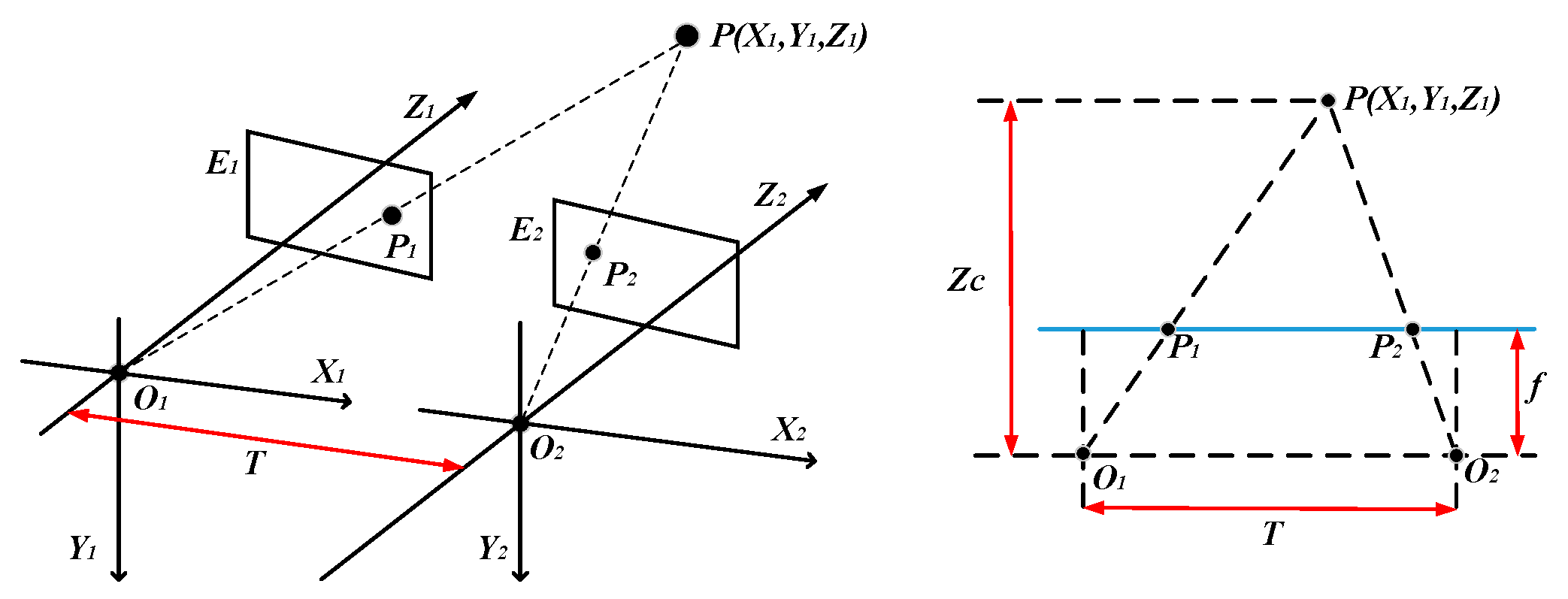
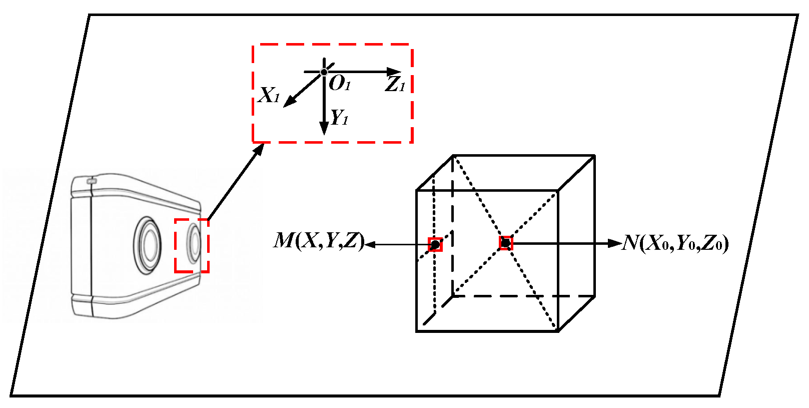
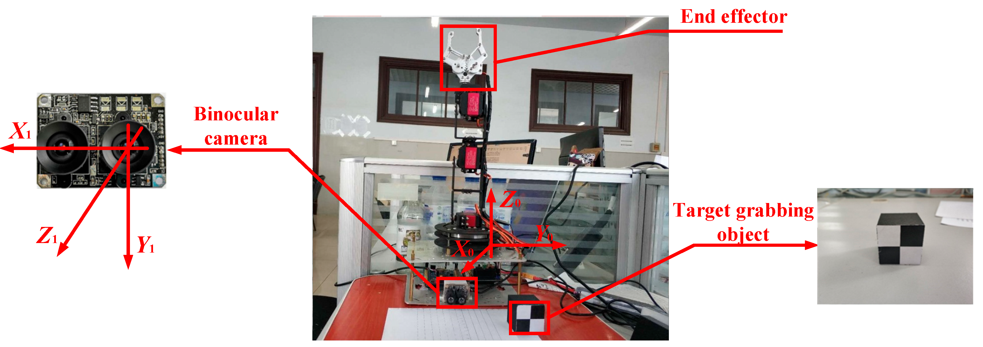
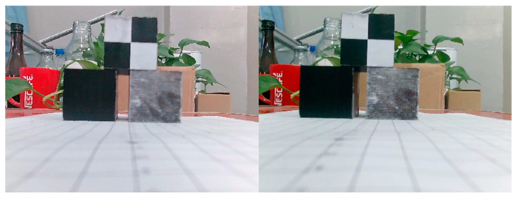
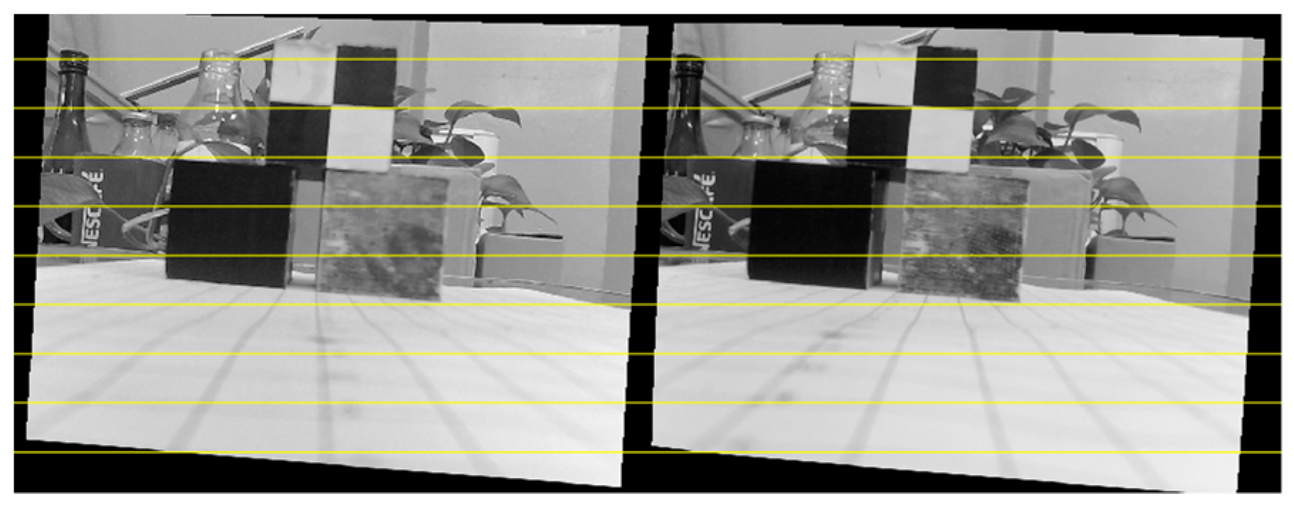
2.1. Binocular Vision Positioning Principle

The target-grabbing object is spatially positioned using a parallel binocular camera. The positioning principle is shown in Figure 1.

In the picture, the coordinate system O₁X₁Y₁Z₁ is the left camera coordinate system; P is a point in the left camera coordinate system with coordinates (X₁, Y₁, Z₁); O₂X₂Y₂Z₂ is the right camera coordinate system; E₁ and E₂ are the left and right camera imaging planes, respectively; T is called the baseline distance, which represents the distance between the optical centers of the two cameras; the distance from the optical center to the imaging plane is the camera focal length, indicated by the symbol f; and P₁ and P₂ are the image points of the P on the imaging planes E₁ and E₂, respectively. The coordinates of P₁ in the left image coordinate system are (u₁, v₁), and the coordinates of P₂ in the right image coordinate system are (u₂, v₂). In accordance with the corresponding geometric relationship, the coordinate of the P point in the left camera coordinate system are as in Equation (1); the parameters u₀, v₀, f_x, f_y, and T are determined via camera calibration methods.

$$\{\begin{array}{l}{X}_c=\frac{T(u_1-u_0)}{u_1-u_2}\\ Y_c=\frac{T{f}_x(v_1-v_0)}{f_y(u_1-u_2)}\\ Z_c=\frac{T{f}_x}{u_1-u_2}\end{array}$$

(1)

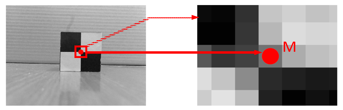
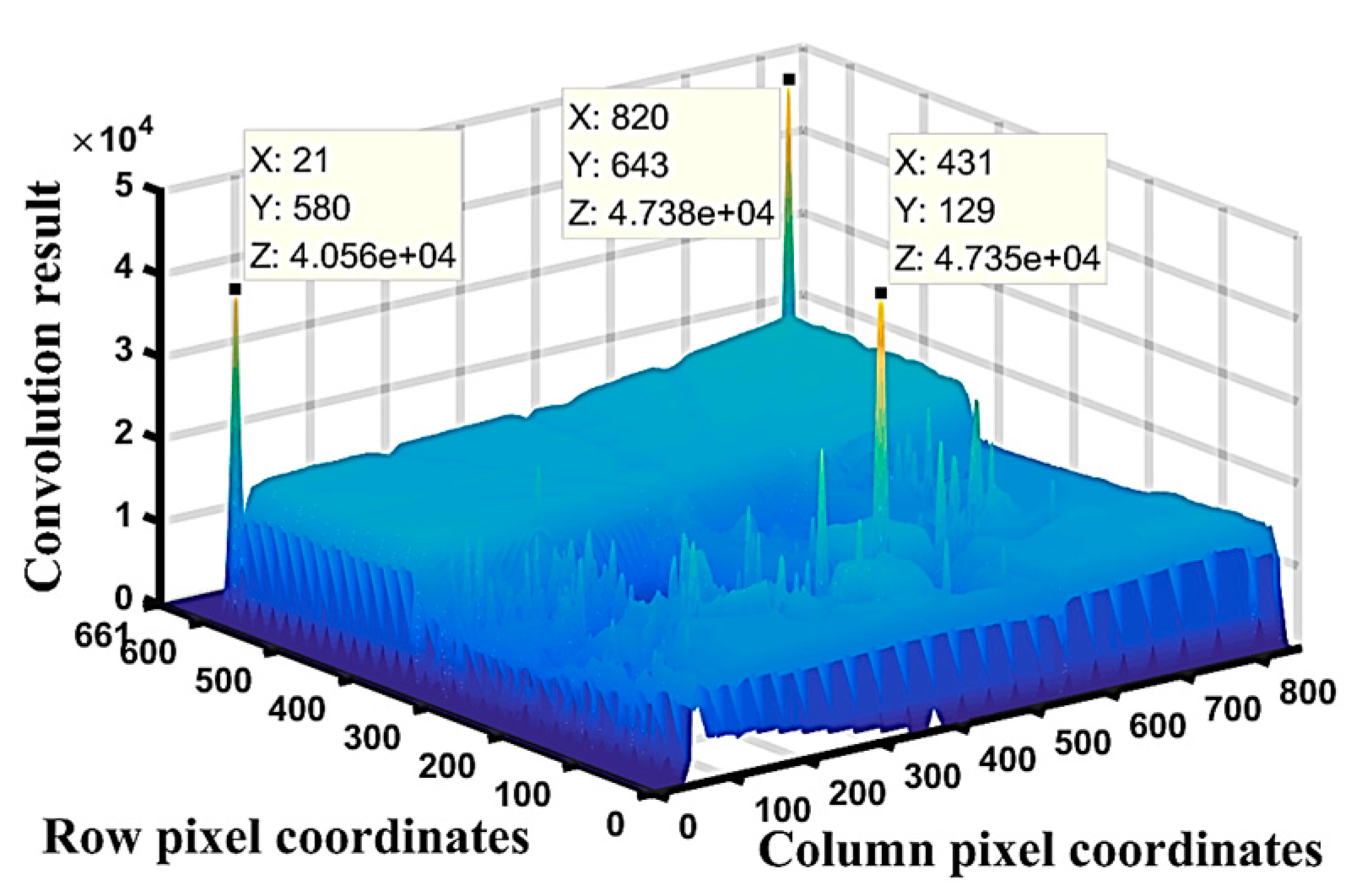
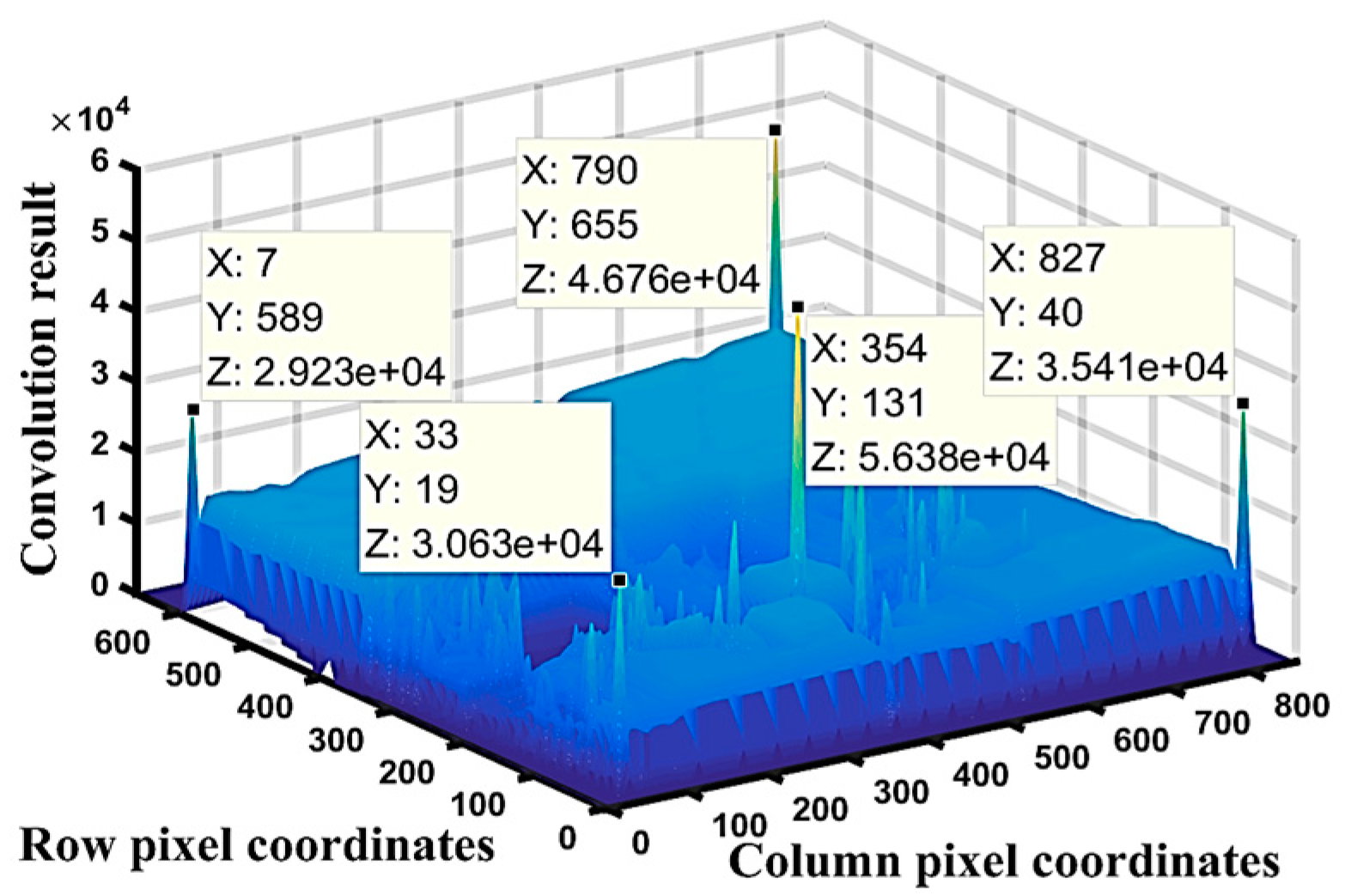
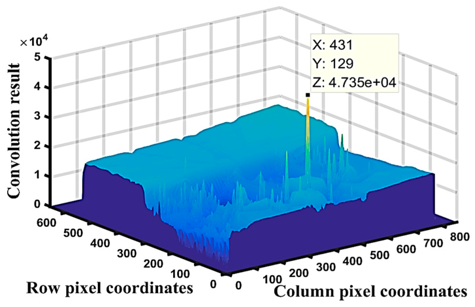
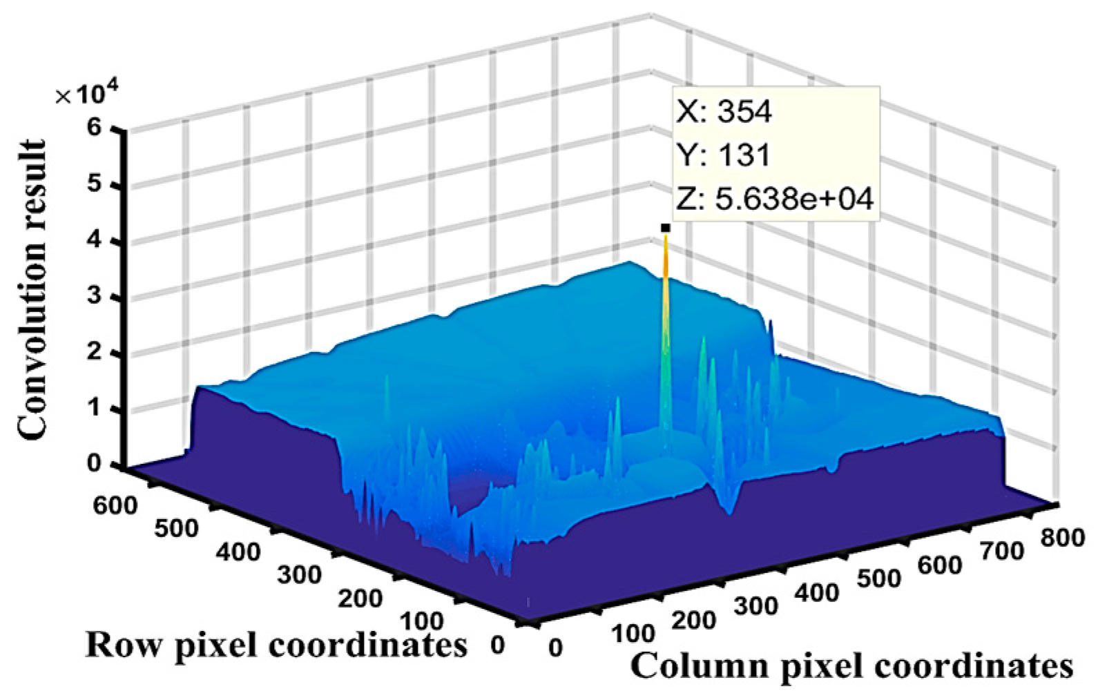
2.2. Target Object Extraction

The target object is a cube with a side length of 40 mm, and its front plane is perpendicular to the optical axis of the camera. The positional relationship between the target object and the camera is shown in Figure 2. It can be seen from the figure the position of the centroid of the target object is the moving target position of the end effector of the robotic arm.

Point M is the front plane center of the target object, whereas point N is the centroid of the target object; the coordinates of the points M and N in the left camera coordinate system are (X, Y, Z) and (X₀, Y₀, Z₀). The relationship between M and N is shown in Equation (2), where l is the side length of the target object.

$$\{\begin{array}{l}{X}_0=X\\ Y_0=Y\\ Z_0=Z+l/2\end{array}$$

(2)

In accordance with the above analysis, the positioning of the centroid of the target object can be transformed into the positioning of point M. Point M is set as the target feature point of the study. The gray scale distribution of the image near the target feature point is shown in Figure 3.

The gray value matrix of the image in the red frame in Figure 4 is K, which is defined as follows:

$$K=\left[\begin{array}{ccc}A& AB& B\\ AC& O& BD\\ C& CD& D\end{array}\right]=\left[{}_{}\begin{array}{ccccccccc}{a}_{11}& \cdots & a_{1n}& a{b}_{11}& \cdots & a{b}_1{}_m& b_{11}& \cdots & b_{1n}\\ ⋮& \ddots & ⋮& ⋮& \ddots & ⋮& ⋮& \ddots & ⋮\\ a_{n1}& \cdots & a_{nn}& a{b}_{n1}& \cdots & a{b}_{nm}& b_{n1}& \cdots & b_{nn}\\ a{c}_{11}& \cdots & a{c}_1{}_n& o_{11}& \cdots & o_{1m}& b{d}_{11}& \cdots & b{d}_{1n}\\ ⋮& \ddots & ⋮& ⋮& \ddots & ⋮& ⋮& \ddots & ⋮\\ a{c}_{m1}& \cdots & a{c}_{mn}& o_{m1}& \cdots & o_{mm}& b{d}_{m1}& \cdots & b{d}_{mn}\\ c_{11}& \cdots & c_{1n}& c{d}_{11}& \cdots & c{d}_{1m}& d_{11}& \cdots & d_{1n}\\ ⋮& \ddots & ⋮& ⋮& \ddots & ⋮& ⋮& \ddots & ⋮\\ c_{n1}& \cdots & c_{nn}& c{d}_{n1}& \cdots & c{d}_{nm}& d_{n1}& \cdots & d_{nn}\end{array}\right].$$

(3)

In Equation (3), the matrix AB, AC, BD, and CD is the gray value matrix of the black and white boundary in the image, where m is much smaller than n. In the ideal case, the values of the elements in matrix A and matrix D are 0, whereas those in matrix B and matrix C are 255. The gray value of the pixel changes uniformly at the black and white boundary in the image. The values of the elements in matrices AC and BD gradually increase from top to bottom, whereas those in matrices AB and BD gradually increase from left to right. The target feature point is located in the matrix O. It should be noted that, if the extracted target feature point is located in the region O, then the extraction can be considered successful because m is a small positive integer. Image convolution operation is used to enlarge the feature point feature to achieve target point extraction. The convolution process is as follows:

$$d(x,y)={\displaystyle \sum _{s=1}^{2b+1}{\displaystyle \sum _{t=1}^{2b+1}w(s,t)y(x-s+b+1,y-t+b+1)}}.$$

(4)

In Equation (4), w (s, t) is the convolution kernel of the image convolution operation and is defined as Equation (5), and b is a positive integer. y (x, y) is the gray matrix of the input image, and d (x, y) is the convolution result output matrix, which is the same size as the input image gray matrix.

$$w\left(s,t\right)=\left[\begin{array}{ccc}E& EF& F\\ EG& I& FH\\ G& GH& H\end{array}\right]=\left[\begin{array}{ccccccc}{e}_{11}& \cdots & e_{1b}& e{f}_{11}& f_{11}& \cdots & f_{1b}\\ ⋮& \ddots & ⋮& ⋮& ⋮& \ddots & ⋮\\ e_{b1}& \cdots & e_{bb}& e{f}_{b1}& f_{b1}& \cdots & f_{bb}\\ e{g}_{11}& \cdots & e{g}_{1b}& i& f{h}_{11}& \cdots & f{h}_{1b}\\ g_{11}& \cdots & g_{1b}& g{h}_{11}& h_{11}& \cdots & h_{1b}\\ ⋮& \ddots & ⋮& ⋮& ⋮& \ddots & ⋮\\ g_{b1}& \cdots & g_{bb}& g{h}_{b1}& h_{b1}& \cdots & h_{bb}\end{array}\right]=\left[\begin{array}{ccccccc}-1& \cdots & -1& 1& 1& \cdots & 1\\ ⋮& \ddots & ⋮& ⋮& ⋮& \ddots & ⋮\\ -1& \cdots & -1& 1& 1& \cdots & 1\\ 1& \cdots & 1& 1& 1& \cdots & 1\\ 1& \cdots & 1& 1& -1& \cdots & -1\\ ⋮& \ddots & ⋮& ⋮& ⋮& \ddots & ⋮\\ 1& \cdots & 1& 1& -1& \cdots & -1\end{array}\right]$$

(5)

The pixel in the original image that maximizes the convolution result is the target feature extraction point, and can be extracted based on the distribution of gray values around the target point. The extraction process is as follows:

$$A=\max (d(x,y)),$$

(6)

$$d(x_0,y_0)=A.$$

(7)

The solution to Equation (7) is the position coordinate of the target feature point in the image. However, the above method cannot be applied when the target object is placed by 90° rotation. By combining the two ways of placing the target object, the target point extraction method is changed to Equations (8)–(12).

$$u(s,t)=rot90°(w(s,t))$$

(8)

$$f(x,y)={\displaystyle \sum _{s=1}^{2b+1}{\displaystyle \sum _{t=1}^{2b+1}u(s,t)y(x-s+b+1,y-t+b+1)}}.$$

(9)

$$p(x,y)=\mathrm{abs}\left(d(x,y)\right)+\mathrm{abs}\left(f(x,y)\right)$$

(10)

$$C=\max (p(x,y))$$

(11)

$$p(x_2,y_2)=C$$

(12)

The definitions of the parameters in the above process are consistent with the previous ones. The solution to Equation (12) is the position coordinate in the image where the target point is located.

2.3. Multi-DOF Robotic Arm Trajectory Planning Method

Genetic algorithm is a method derived from the theory of evolution that searches for the optimal solution by simulating the natural evolution process [19]. It has always been the most important algorithm for solving constrained optimization problems [20]. Further, the trajectory planning method based on joint space has a smaller amount of calculation because it can avoid the inverse kinematics process and directly obtain the optimal motion angle value of each joint compared with the trajectory planning method based on Cartesian space, which is convenient to implement in actual engineering. Thus, we use the genetic algorithm to plan the trajectory of the multi-DOF robotic arm in joint space to improve the working efficiency of the robotic arm. The goal is to take the robotic arm to grasp the target object with the shortest moving time and the minimum grab error. Each joint motion variable is a parameter to be optimized.

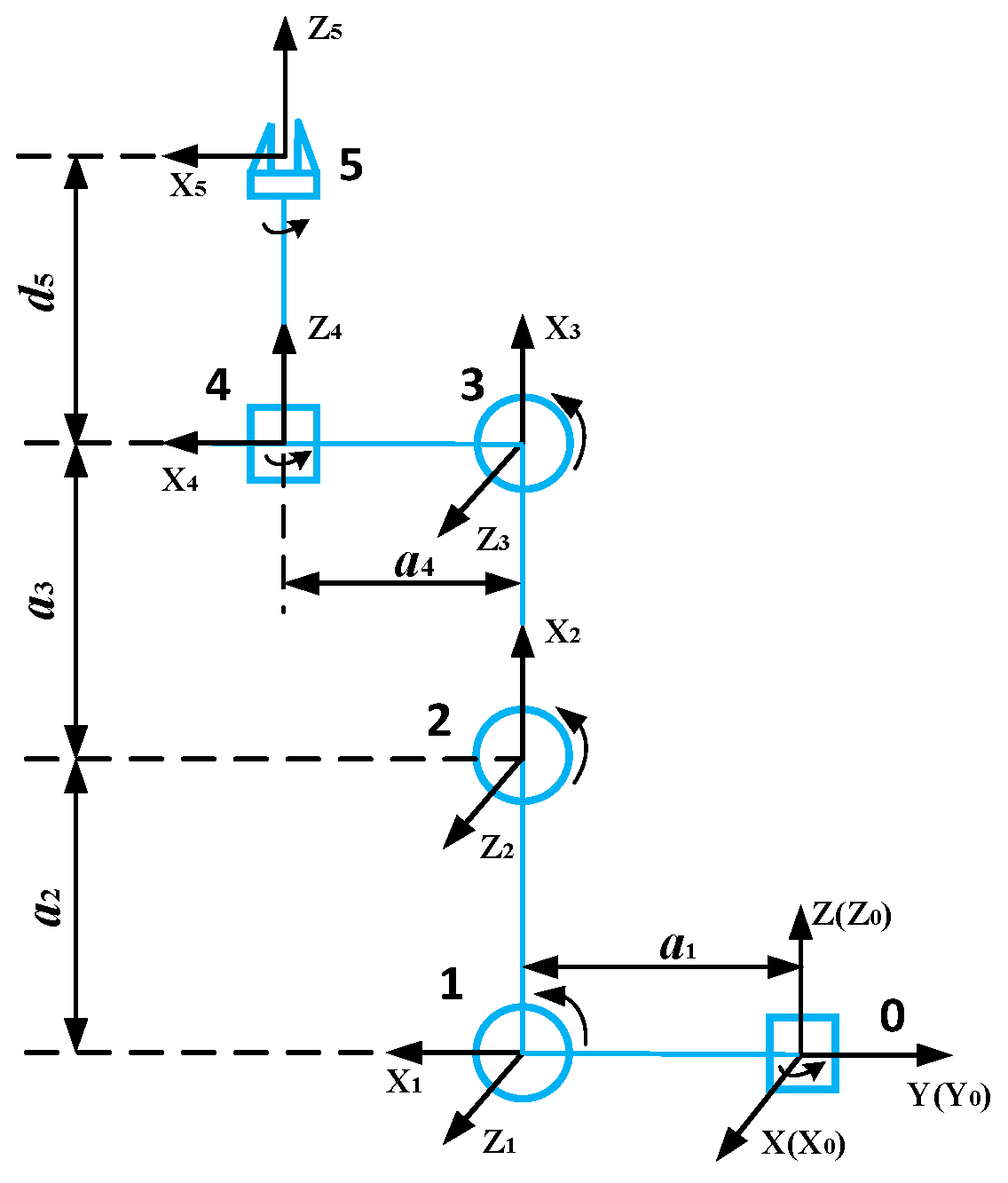
2.3.1. Multi-DOF Robotic Arm Kinematics Modeling

The robotic arm used in this study consists of five joints and one end effector. The kinematics of the robotic arm is modeled using the classical Denavit-Hartenberg (D-H) method. Figure 4 shows the kinematics model of the robotic arm as well as the joint coordinate system and parameter definitions.

Define the previous joint coordinate system as n and the latter joint coordinate system as n + 1. The transformation matrix ⁿT_n+1 between the two coordinate systems is as follows:

$${}^{n}T_{n+1}=(\begin{array}{l}\cos {\theta }_{n+}{}_1\\ \sin {\theta }_{n+}{}_1\\ 0\\ 0\end{array}\begin{array}{c}\\ \\ \\ \end{array}\begin{array}{ccc}{-\sin \mathsf{\theta }}_{n+}{}_1{\cos \mathsf{\alpha }}_{n+1}& {\sin \mathsf{\theta }}_{n+}{}_1{\sin \mathsf{\alpha }}_{n+}{}_1& \\ {\cos \mathsf{\theta }}_{n+}{}_1{\cos \mathsf{\alpha }}_{n+}{}_1& {-\cos \mathsf{\theta }}_{n+}{}_1{\sin \mathsf{\alpha }}_{n+}{}_1& \\ {\sin \mathsf{\alpha }}_{n+}{}_1& {\cos \mathsf{\alpha }}_{n+}{}_1& \\ 0& 0& \end{array}\begin{array}{l}{a}_{n+}{}_1\cos {\theta }_{n+}{}_1\\ a_{n+}{}_1\sin {\theta }_{n+}{}_1\\ d_{n+1}\\ 1\end{array}),$$

(13)

where θ_i represents the angle between the two axes of X_i and X_i+1, with the right rotation around the Z_i axis set to the positive direction; d_i represents the distance between the adjacent joints X_i and the X_i+1 axis; a_i represents the distance between the adjacent joints Z_i and the Z_i+1 axis; and α_i represents the angle between the two axes of Z_i and Z_i+1, with the right rotation around the X_i axis set to the positive direction. According to the established kinematic model of the robotic arm, the conversion matrix from base coordinate system 0 to end effector coordinate system 5 can be obtained as follows:

$${}^{0}T_5={}^{0}T_1({\theta }_1){}^{1}T_2({\theta }_2){}^{2}T_3({\theta }_3){}^{3}T_4({\theta }_4)=\left(\begin{array}{cccc}{n}_x& o_x& a_x& p_x\\ n_y& o_y& a_y& p_y\\ n_z& o_z& a_z& p_z\\ 0& 0& 0& 1\end{array}\right),$$

(14)

where (p_x, p_y, p_z)^T is the position coordinate of the end effector of the robotic arm that we care about at the base coordinate of the arm base. The calculated end effector coordinates are as in Equation (15).

$$\{\begin{array}{l}{p}_x=\cos {\theta }_1\times \left(a_3\cos ({\theta }_2+{\theta }_3)+a_2\cos {\theta }_2+a_4\cos ({\theta }_2+{\theta }_3+{\theta }_4)+d_5\sin ({\theta }_2+{\theta }_3+{\theta }_4)+a_1\right)\\ p_{\mathrm{y}}=\sin {\theta }_1\times (a_3\cos ({\theta }_2+{\theta }_3)+a_2\cos {\theta }_2+a_4\cos ({\theta }_2+{\theta }_3+{\theta }_4)+d_5\ast \sin ({\theta }_2+{\theta }_3+{\theta }_4)+a_1)\\ p_z=d_5\cos ({\theta }_2+{\theta }_3+{\theta }_4)-a_2\sin {\theta }_2-a_3\sin ({\theta }_2+{\theta }_3)-a_2\sin ({\theta }_2+{\theta }_3+{\theta }_4)\end{array}$$

(15)

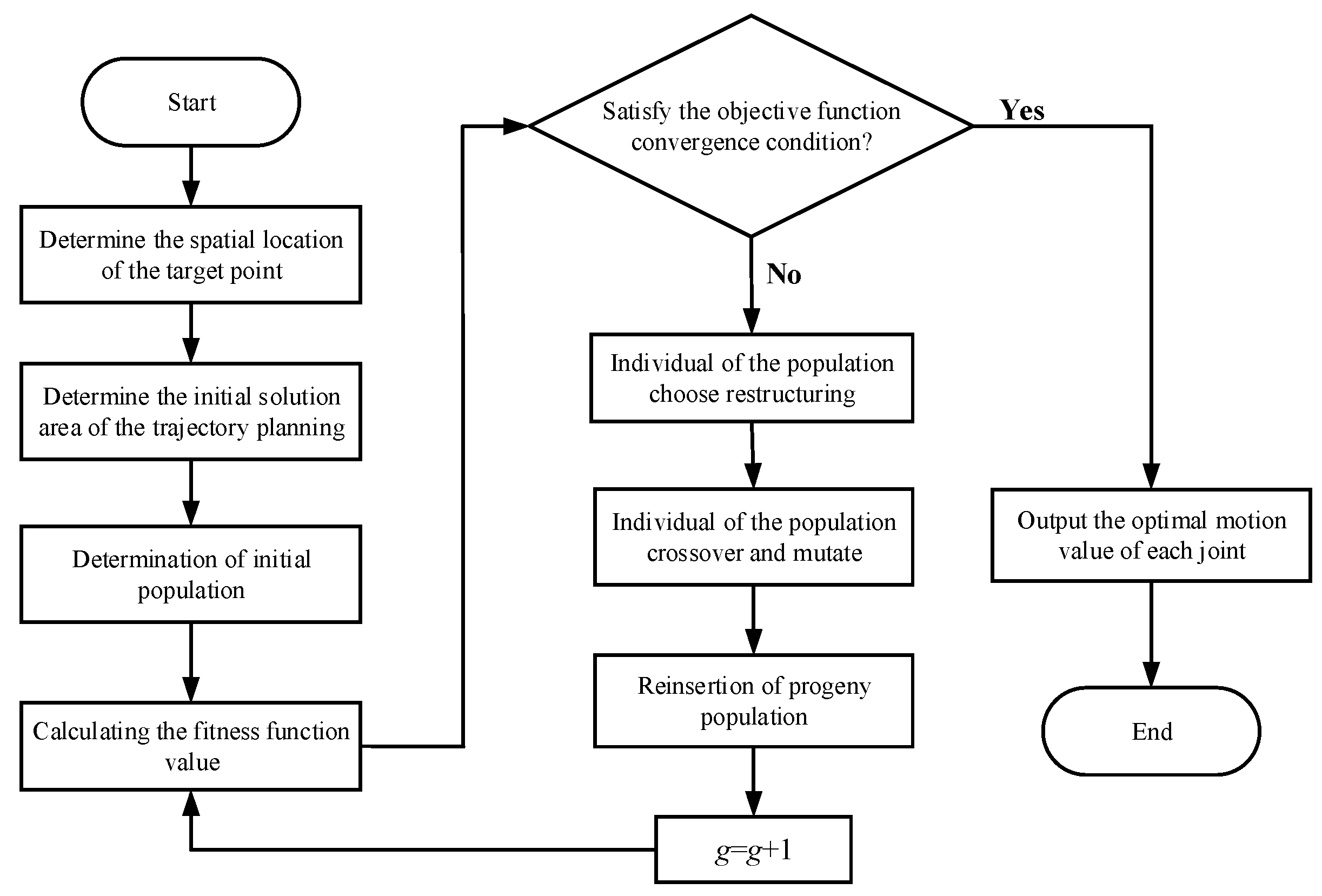
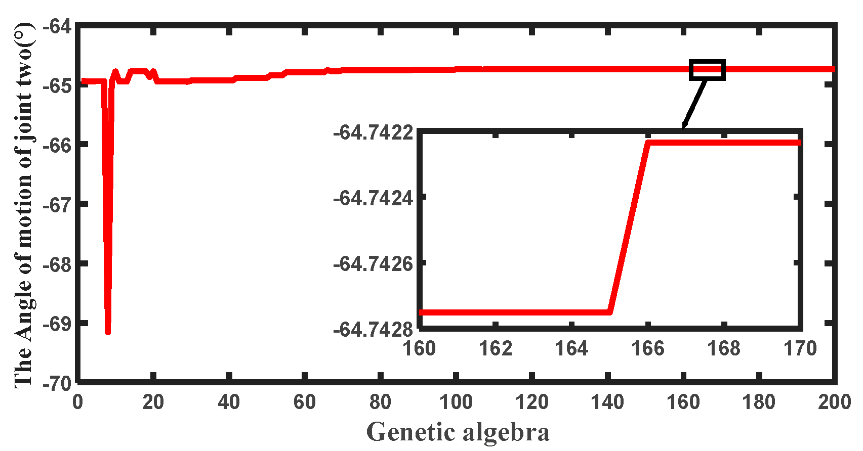
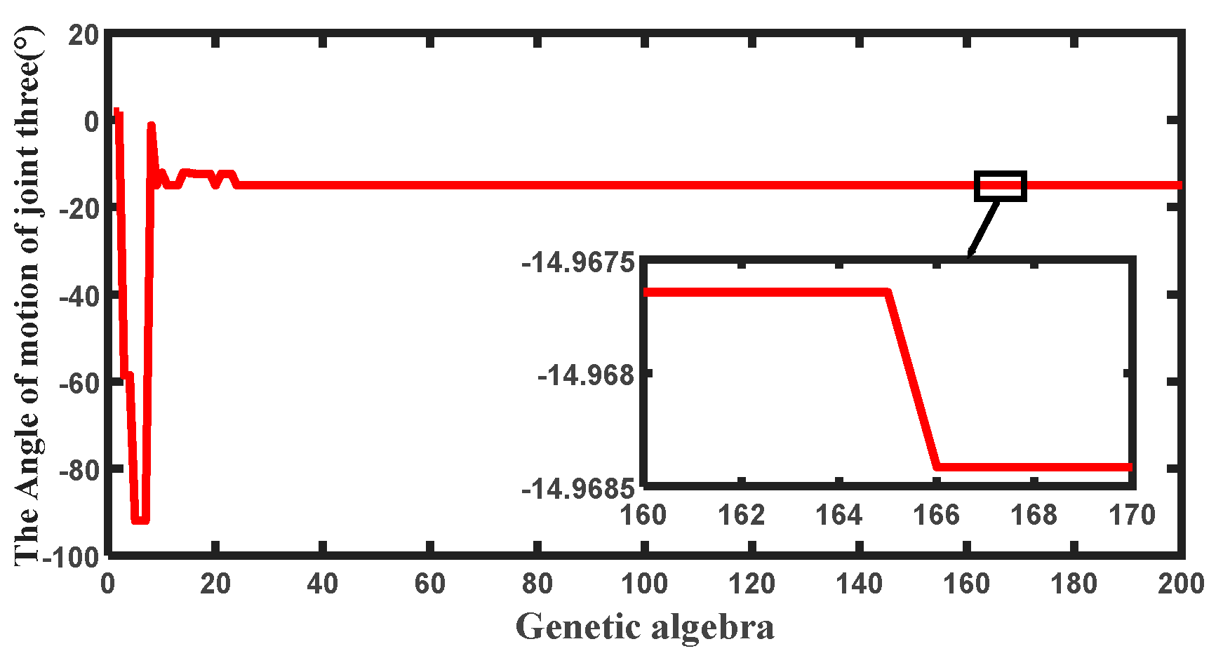
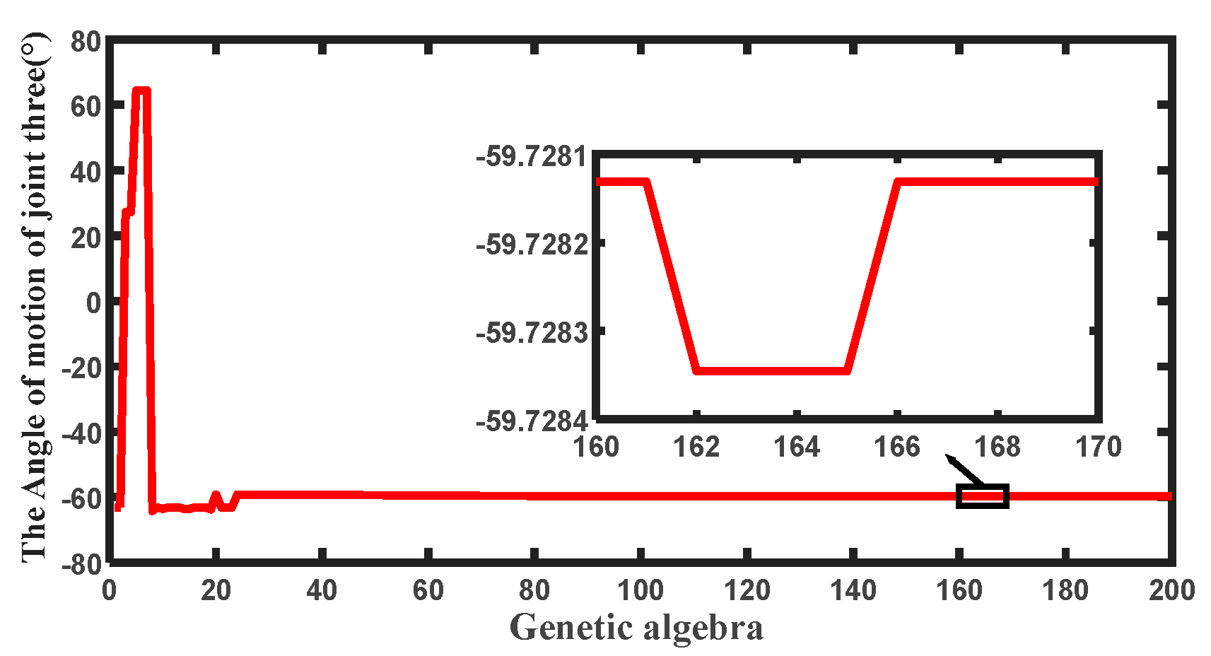
2.3.2. Robotic Arm Motion Trajectory Planning Method Based on Genetic Algorithm

According to the optimization goal, the objective function fit of the trajectory planning can be set as follows:

$$Fit=\{\begin{array}{l}\alpha \cdot max(\left|C_1/{\omega }_1\right|,\left|C_2/{\omega }_2\right|,\left|C_3/{\omega }_3\right|,\left|C_4/{\omega }_4\right|)+\beta \cdot F_1\hspace{1em}\hspace{1em}{l}_{obj}\le l_{cur}\le l_{\max }\\ \alpha \cdot max(\left|C_1/{\omega }_1\right|,\left|C_2/{\omega }_2\right|,\left|C_3/{\omega }_3\right|,\left|C_4/{\omega }_4\right|)+\beta \cdot F_1+\gamma \hspace{1em}\hspace{1em}\hspace{1em}else\end{array},$$

(16)

where ω₁, ω₂, ω₃, and ω₄ represent the angular velocity of the first four joints of the robotic arm; β and α are the weight coefficients of the optimization function; C₁, C₂, C₃, and C₄ are the corresponding joint rotation angles during the motion of the robotic arm; and F₁ is the distance error function, which is defined as the spatial distance between the end effector coordinates (x, y, z) and the target point (x_f, y_f, z_f) during the motion of the robotic arm, as shown in the following equation:

$$F_1=\sqrt{{\left(x-x_f\right)}^2+{\left(y-y_f\right)}^2+{\left(z-z_f\right)}^2}.$$

(17)

The constraints of the trajectory planning process are as follows:

(1)

Joint constraint

$$C_2+C_3+C_4=\kappa .$$

(18)

(2)

Connecting rod constraint

$$l_{obj}\le l_{cur}\le l_{\max }.$$

(19)

In the joint constraint, κ is the rotation angle of the end connecting rod of the robotic arm from the initial position to the end position in the base coordinate system 0. The angle varies from −160° to 160°. The sum of the rotation angles of the joints 2, 3, and 4 is equal to the rotation angle of the end connecting rod. The motion of joint 1 is not constrained by the joints. In the connecting rod constraint, l_obj, l_cur, and l_max are the distances from the target space point to the origin of the base coordinate system of the robotic arm, the real-time distance between the end effector and the origin of the base coordinate system during the motion of the robotic arm, and the distance between the end effector and the origin of the base coordinate system in the upright position, respectively. The trajectory planning process needs to meet the link constraints. Otherwise, the end effector cannot reach the target point position [21].

To highlight the importance of the error function in the objective function, the optimization weight coefficient should satisfy β >> α. When the trajectory planning result does not satisfy the constraint, the penalty term γ is added after the objective function to increase the objective function value and reduce the individual fitness of the population. When the change of the objective function value satisfies the convergence condition, the optimization process ends, and the optimal motion angle of each joint is output. The trajectory planning process based on genetic algorithm is shown in Figure 5.

3. Results

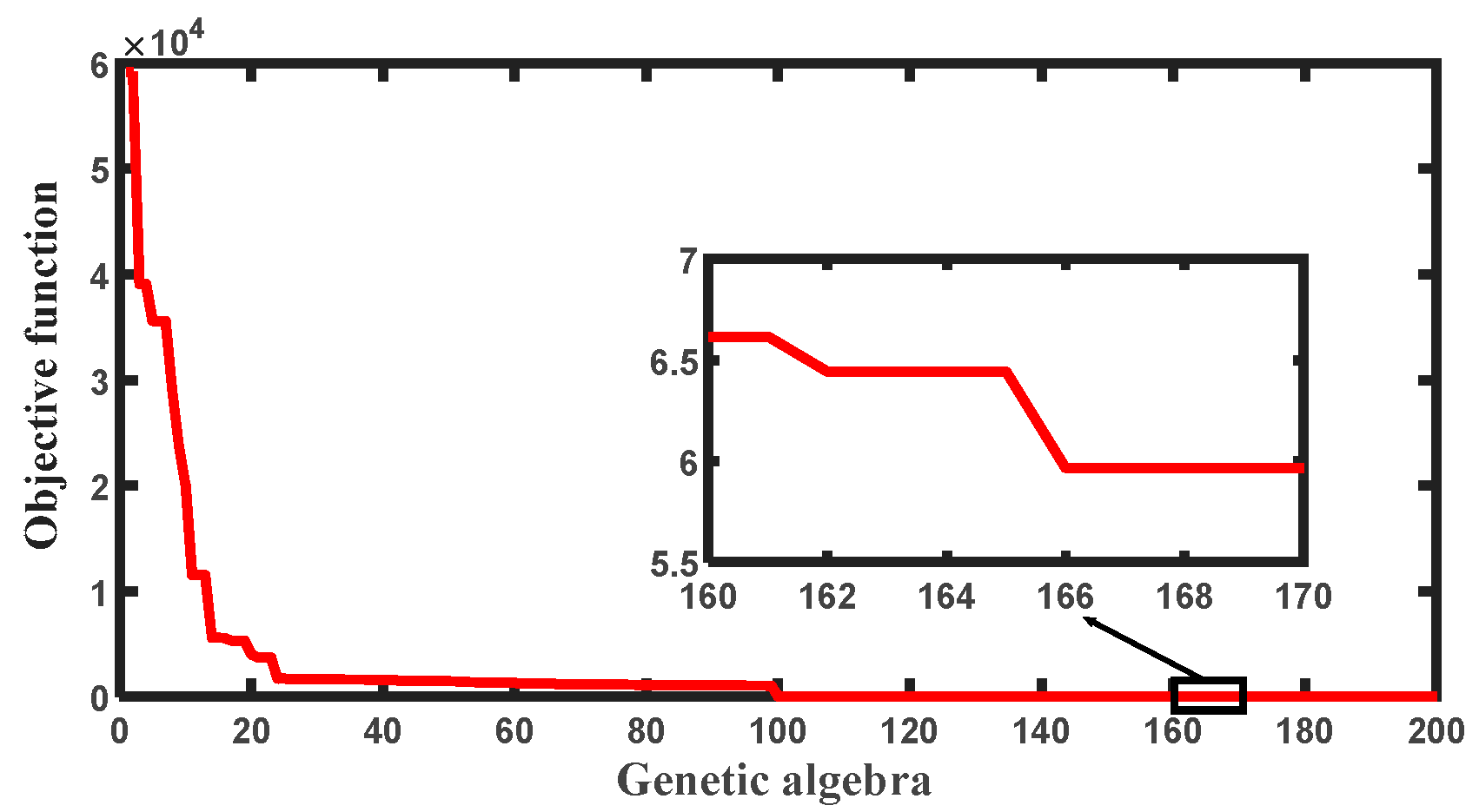
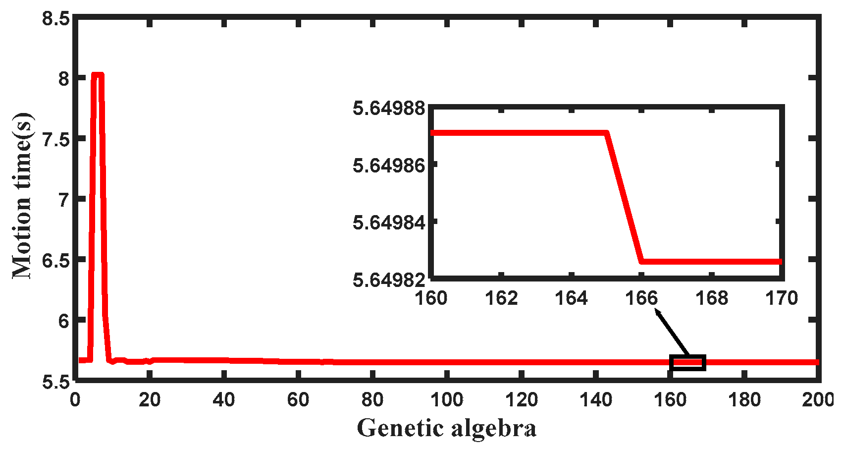
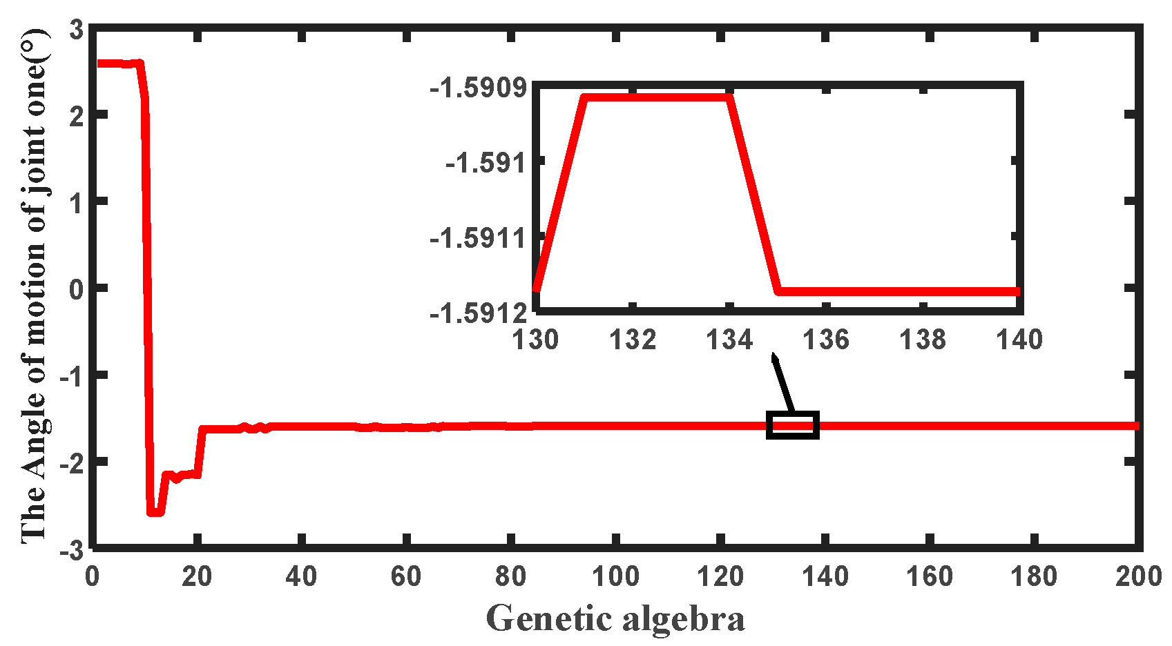
3.1. Simulation Verification of Multi-DOF Robotic Arm Trajectory Planning Method

The D-H parameters of the robotic arm, the initial angle values of the joints, and the range of motion angles are shown in

Table 1. Multiple Degree of Freedom (Multi-DOF) robotic arm Denavit-Hartenberg (D-H) parameter table.

Joint Number	Initial Angle of θi (°)	Range of θi (°)	di (mm)	ai (mm)	αi (°)
1	−90	−135~135	0	10	−90
2	−90	−90~90	0	104	0
3	0	−135~135	0	96	0
4	90	−135~135	0	27	90
5	0	−180~180	137	0	0

.

Table 1 shows that the relationship between θ₁, θ₂, θ₃, and θ₄ and the corresponding joint rotation angles C₁, C₂, C₃, and C₄ during the movement of the arm is as follows:

$$\{\begin{array}{l}{\theta }_1=C_1-{90}^{\circ }\\ {\theta }_2=C_2-{90}^{\circ }\\ {\theta }_3=C_3\\ {\theta }_4=C_4+{90}^{\circ }\end{array}.\{\begin{array}{l}{\theta }_1=C_1-{90}^{\circ }\\ {\theta }_2=C_2-{90}^{\circ }\\ {\theta }_3=C_3\\ {\theta }_4=C_4+{90}^{\circ }\end{array}.$$

(20)

The parameters of the genetic algorithm selected in this study and the meaning of the parameters are shown in

Table 2. Genetic algorithm related parameter list.

Parameter	Numerical Value
Population size (N)	100
Maximum genetic algebra (gmax)	200
Recombination crossover probability (Pc)	0.7
Mutation probability (Pm)	0.5
Optimization weight coefficient (α)	1
Optimization weight coefficient (β)	100
Penalty parameter (γ)	1000
Objective function convergence accuracy	10−5

.

The proposed trajectory planning method is simulated. Let the coordinates of the target point be (8, 288, −25), ω₁ = ω₂ = ω₃ = ω₄ = 0.2 rad/s. The simulation results of the objective function, motion time, distance error, and the angle of motion of each joint with the increase of genetic algebra are shown in Figure 6, Figure 7, Figure 8, Figure 9, Figure 10, Figure 11 and Figure 12.

The optimum motion angle values for each joint that can be obtained from the simulation results are shown in

Table 3. Optimal motion angle of each joint.

Joint Number	1	2	3	4
Ci (°)	−1.59117	−64.7422	−14.9684	−59.7281

.

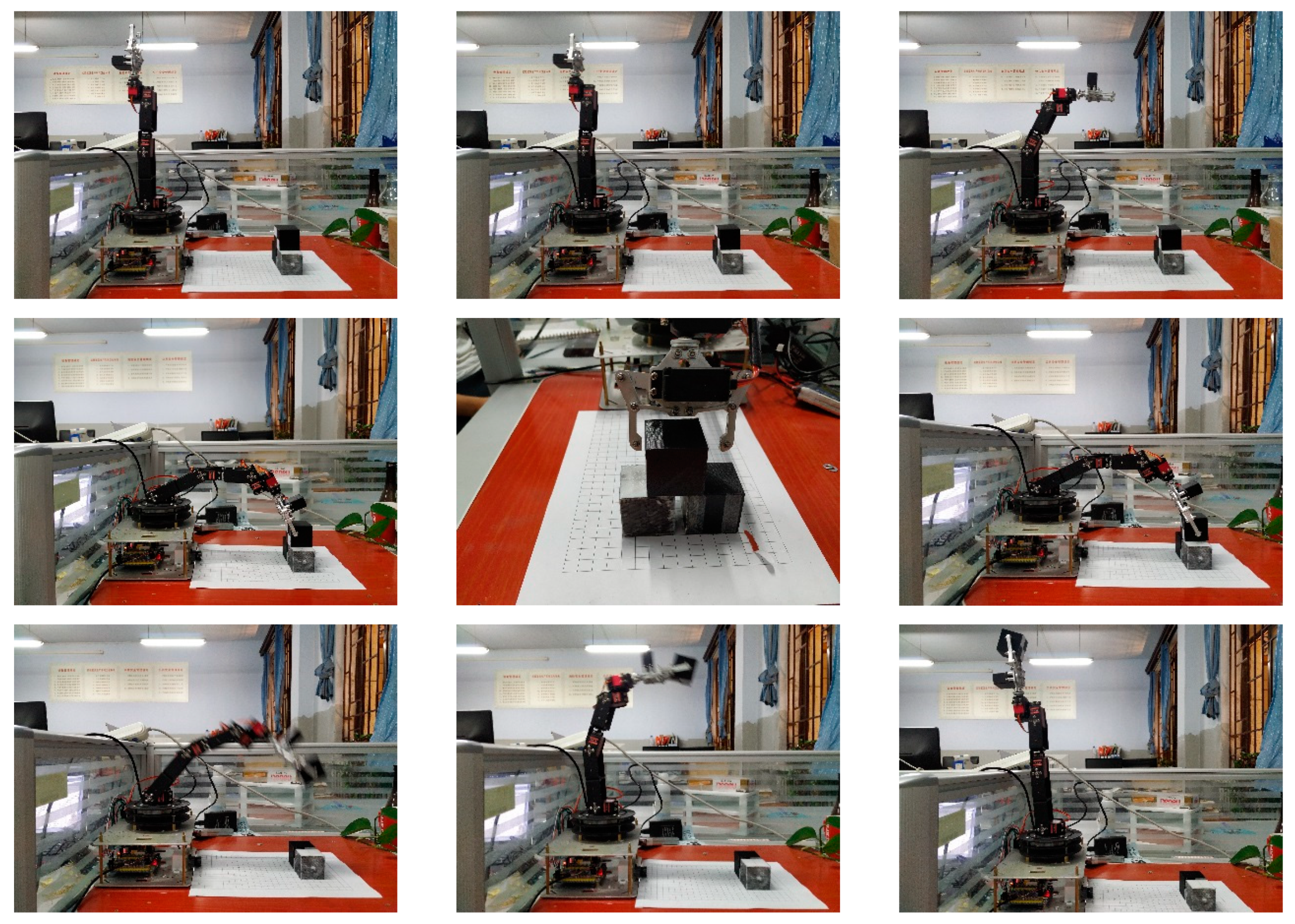
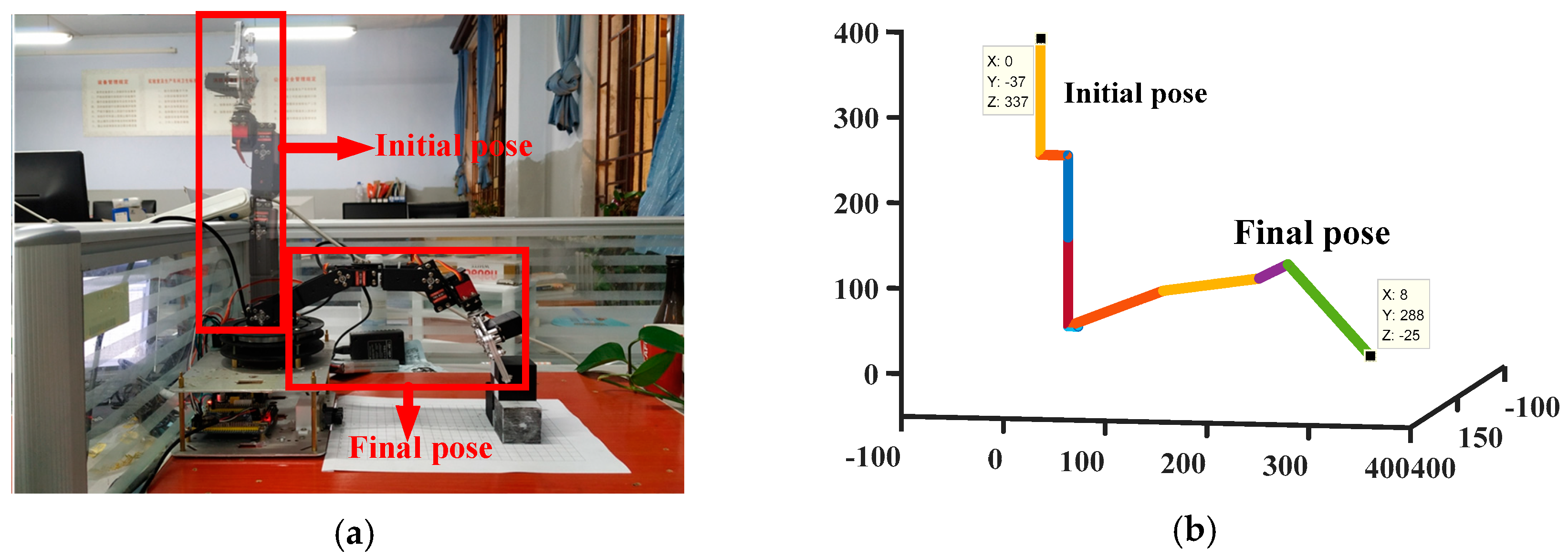
3.2. Experimental Verification of Autonomous Operation Method for Multi-DOF Robotic Arm

A small object prototype model is built to verify the practicability and correctness of the proposed robotic autonomous operation method. The prototype model is shown in Figure 13.

The conversion relationship between the target point coordinate (X, Y, Z) in the camera coordinate system and the centroid coordinate (X₂, Y₂, Z₂) of the target object in the robotic arm coordinate system is determined via the following experimental calibration:

$$\{\begin{array}{l}{X}_2=Z+118\\ Y_2=-X-8\\ Z_2=-Y-70\end{array}.$$

(21)

The target object is placed in a manner that its center of mass is located in the base coordinate system (288, −8, −25). From Equation (21), the coordinates of the target point are (0, −45, 170) in the left camera coordinate system. A binocular camera is used to obtain the target grab image, as shown in Figure 14.

Epipolar line rectification is performed on the left and right images. The corrected output image is shown in Figure 15.

A convolution operation is performed on the image corrected by epipolar line rectification. The distribution of convolution results is shown as follows.

The pixel points at the vertices of the image after the epipolar line rectification enlarge the convolution result; the points are marked in Figure 16 and Figure 17. This situation occurs because of the large difference in the distribution of gray values near the pixel points at the vertices of the image. The convolution result of the boundary pixel points of the image is set to zero to eliminate the interference of the pixel points on the vertices of the original image to the target point extraction. The image convolution results after adjustment are shown in Figure 18 and Figure 19.

After adjustment, the pixel point with the largest convolution result is calibrated in the original image to complete the target point extraction. The extraction result is shown in Figure 20. In the complex background, the method proposed can be used to extract the target point accurately, and it has a good extraction effect.

The coordinates of the target point extracted from the left and right images are brought into Equation (1). The spatial coordinates of the target point are (14.26, −44.33, 159.16). In comparison with the actual coordinates (0, −45, 170), a large error exists in the positioning result. To determine the range of the positioning error in the common field of view of the binocular camera, the target object positioning experiment was performed multiple times in the depth of field of 70 mm to 200 mm. The experimental result is that, in the left camera coordinate system, the positioning error of the target point in the Y₁ direction satisfies the system positioning error requirement, but a large positioning deviation occurs in the X₁ and Z₁ directions. When the target point moves in the Z₁ direction, the overall deviation value becomes increasingly large as the depth of field increases. Therefore, the relationship between the depth of field and the target position deviation value is established, and the measurement result is compensated by the error fitting method. In this manner, the positioning error of the target point is controlled within the ideal range.

The positioning result after processing is compared with the actual position of the target point to obtain the relative error of the positioning. The final positioning results are shown in

Table 4. Positioning and relative positioning errors.

Error	Maximum (mm)	Minimum (mm)
X1	8.02	0.004
Y1	5.5	0.002
Z1	6.03	0.003
Positioning relative error	6.60%	1.19%

. The relative error of positioning is expressed by F₂ and defined as Equation (22). The target point positioning coordinates and the actual coordinates are (X_a, Y_a, Z_a) and (X, Y, Z), respectively.

$$F_2=\frac{\sqrt{{(X-X_a)}^2+{(Y-Y_a)}^2+{(Z-Z_a)}^2}}{\sqrt{X^2+Y^2+Z^2}}$$

(22)

The joints of the robotic arm motion are set in accordance with the corresponding angles in Table 3. The end effector can reach the vicinity of the centroid point of the target object and grab the target object. The entire grab process is shown in Figure 21.

The actual motion trajectory of the robotic arm is compared with the simulated motion trajectory, as shown in Figure 22. The experimental results are consistent with the simulation results, thereby proving the correctness of the proposed method.

To determine the error of the robotic arm grabbing and the autonomous performance, the position of the target object is changed multiple times within the effective working area of the system. As a result, the experiments of the robotic arm autonomous operation are performed 100 times. The distance error between the final end effector and the centroid of the target object and the number of successful grabs of the target object are recorded. The error of the grabbing mainly considers the error in the direction of Y₀ and Z₀. The experimental results are shown in

Table 5. Experimental results of robotic arm autonomous operation.

List	Y0	Z0
Maximum error (mm)	30	21
Minimum error (mm)	1	2
Error mean (mm)	14.0
Error variance (mm)	6.5
Grab success rate	83%

.

4. Discussions

Industry 4.0 is the current industrial revolution and robotics is an important factor for carrying out high dexterity manipulations [22]. With the development of society, robotic arm technology has been widely used. In recent years, the demand for the intelligent robotic arm has been increasing. How to make the robotic arm capable of autonomous operation has gradually become a research hotspot [23]. With the rapid development of computer vision technology, the robotic arm have the ability to sense the environment by combining vision technology, and it is beginning to have autonomous operation capabilities. However, there are still some serious problems. In terms of target extraction, the traditional method of object extraction based on image segmentation, it has the advantages of less computation and easy implementation. However, this method is extremely demanding on environmental conditions and has low robustness and versatility. It is usually applicable to the situation in which the target object has a single background and fixed environmental conditions, because it is often necessary to re-acquire the method-related parameters when the environmental conditions of the target object change. The currently used target object extraction methods based on deep learning have the advantages of insensitivity to changes in environmental conditions, high extraction accuracy, and good robustness. However, the calculation process is complicated and requires high hardware systems to implement the method. At the same time, this method is not suitable for practical applications because it requires a lot of time to collect and produce a large number of image samples containing the target object to train the entire network model parameters.

A target object extraction method based on extracting target feature points is proposed to address the above problems. It can be seen from the above experimental results that the effect of the extraction of target feature points is good when the target object is in a relatively complex environmental background. The environmental conditions in which the target object is located have changed during experiments, such as the lighting and background placement of disturbing objects. In this case, the target feature points can be successfully extracted in almost every experiment. This shows that the proposed method has the advantages of high extraction accuracy, good robustness, and insensitivity to changes in environmental conditions. At the same time, the target feature point extraction method is based on image convolution operation, which is easy to implement in hardware systems because the amount of calculation is smaller compared with methods such as target object extraction based on machine learning ideas. Therefore, it can be applied in actual engineering.

In the target positioning part, the classic parallel binocular camera positioning method is selected to realize the positioning of the target object because of the existing equipment. However, the relative positioning error is large, and it can be controlled within a reasonable range after compensation. There are more and better target positioning methods now; for example, Sudin, MN et al. proposed a novel localization method consisting of a proposed corner extraction algorithm, namely, the contour intersection algorithm (CIA), as well as a distance estimation algorithm, namely, analytic geometric estimation (AGE), which achieved a better positioning effect compared with other positioning algorithms [24]. In the follow-up research work, more research work will be done on the positioning of target objects.

We choose to plan the trajectory of the robotic arm in the joint space to improve the working efficiency of the robotic arm, because it is convenient to implement in actual engineering. It can be seen from the simulation verification results of the robot arm trajectory planning method that the objective function converges rapidly and, when the objective function converges, the distance error, the motion time, and the motion angle of each joint of the robot arm will converge with the increase of genetic algebra. All relevant simulation parameters converge before the 170th generation. The final coordinates of the end effector are calculated (8.0002, 288.0002, −25.0001) ^T. It can be considered to coincide with the target point. Finally, the grasping error is within 5 × 10⁻³ mm. The simulation results show the correctness and practicability of the proposed motion trajectory planning method for the robotic arm. The experiment was performed 100 times to determine the performance of the proposed autonomous operation method of the robotic arm. The experimental results show that the relative positioning error of the target object can reach 1.19% in the depth of field of 70–200 mm. The average grab error, variance, and grab success rate of the robot arm are 14 mm, 6.5 mm, and 83%, respectively. The main reasons for the failure of the target object being grabbed are as follows:

(1)

An error occurs in the positioning result of the binocular camera for the centroid point of the target object. This error causes the motion planning trajectory of the robot arm to deviate from the theoretical trajectory, thereby affecting the grabbing of the target object;

(2)

The movement of each joint of the robot arm used in the experiment is realized by the steering gear controlled by PWM (Pulse Width Modulation) wave. A deviation occurs between the actual rotation angle of each joint of the robotic arm and the theoretical angle during the motion owing to the insufficient rotation accuracy of the steering gear, which is also the primary reason for failing to grab the target object;

(3)

A measurement error is present in the determination of relevant parameters during the experiment, and this error affects the grabbing of the target object.

The autonomous operation method of the robotic arm proposed in this paper is mainly applied to the grasping and retracting of objects when the target object is in unstable environmental conditions and with limited time resources. It will have a wider range of applications when working with mobile devices; the method has good practical application value because it has the advantages of strong generality, high robustness, and easy implementation.

References

1. Zhao, Y.; Gong, L.; Liu, C.; Huang, Y.; Liu, C. A review of key techniques of vision-based control for harvesting robot. Comput. Electron. Agric. 2016, 127, 311–323. [Google Scholar] [CrossRef]
2. Ling, X.; Zhao, Y.; Gong, L.; Liu, C.; Wang, T. Dual-arm cooperation and implementing for robotic harvesting tomato using binocular vision. Robot. Auton. Syst. 2019, 114, 134–143. [Google Scholar] [CrossRef]
3. Williams, H.A.; Jones, M.H.; Nejati, M.; Seabright, M.J.; Bell, J.; Penhall, N.D.; Barnett, J.J.; Duke, M.D.; Scarfe, A.J.; Ahn, H.S.; et al. Robotic kiwifruit harvesting using machine vision, convolutional neural networks, and robotic arms. Biosyst. Eng. 2019, 181, 140–156. [Google Scholar] [CrossRef]
4. Xiong, J.; He, Z.; Lin, R.; Liu, Z.; Bu, R.; Yang, Z.; Peng, H.; Zou, X. Visual positioning technology of picking robots for dynamic litchi clusters with disturbance. Comput. Electron. Agric. 2018, 151, 226–237. [Google Scholar] [CrossRef]
5. Wu, Q.; Li, M.; Qi, X.; Hu, Y.; Li, B.; Zhang, J. Coordinated control of a dual-arm robot for surgical instrument sorting tasks. Robot. Auton. Syst. 2019, 112, 1–12. [Google Scholar] [CrossRef]
6. Wang, Z.; Li, H.; Zhang, X. Construction waste recycling robot for nails and screws: Computer vision technology and neural network approach. Autom. Constr. 2019, 97, 220–228. [Google Scholar] [CrossRef]
7. Zhang, S.; Wang, Y.; Zhu, Z.; Li, Z.; Du, Y.; Mao, E. Tractor path tracking control based on binocular vision. Inf. Process. Agric. 2018, 5, 422–432. [Google Scholar] [CrossRef]
8. Zhao, S.; Kang, F.; Li, J. Displacement monitoring for slope stability evaluation based on binocular vision systems. Optik 2018, 171, 658–671. [Google Scholar] [CrossRef]
9. Tang, Y.C.; Li, L.J.; Feng, W.X.; Liu, F.; Zou, X.J.; Chen, M.Y. Binocular vision measurement and its application in full-field convex deformation of concrete-filled steel tubular columns. Measurement 2018, 130, 372–383. [Google Scholar] [CrossRef]
10. Liu, W.; Li, X.; Jia, Z.; Li, H.; Ma, X.; Yan, H.; Ma, J. Binocular-vision-based error detection system and identification method for PIGEs of rotary axis in five-axis machine tool. Precis. Eng. 2018, 51, 208–222. [Google Scholar] [CrossRef]
11. Yang, J.; Zhao, Y.; Zhu, Y.; Xu, H.; Wen, L.; Meng, Q. Blind assessment for stereo images considering binocular characteristics and deep perception map based on deep belief network. Inf. Sci. 2019, 474, 1–17. [Google Scholar] [CrossRef] [Green Version]
12. Zhai, Z.; Zhu, Z.; Du, Y.; Song, Z.; Mao, E. Multi-crop-row detection algorithm based on binocular vision. Biosyst. Eng. 2016, 150, 89–103. [Google Scholar] [CrossRef]
13. Rebouças Filho, P.P.; da Silva, S.P.P.; Praxedes, V.N.; Hemanth, J.; de Albuquerque, V.H.C. Control of singularity trajectory tracking for robotic manipulator by genetic algorithms. J. Comput. Sci. 2019, 30, 55–64. [Google Scholar] [CrossRef]
14. Wang, M.; Luo, J.; Yuan, J.; Walter, U. Coordinated trajectory planning of dual-arm space robot using constrained particle swarm optimization. Acta Astronaut. 2018, 146, 259–272. [Google Scholar] [CrossRef]
15. FarzanehKaloorazi, M.H.; Bonev, I.A.; Birglen, L. Simultaneous path placement and trajectory planning optimization for a redundant coordinated robotic workcell. Mech. Mach. Theory 2018, 130, 346–362. [Google Scholar] [CrossRef]
16. Xie, Y.; Wu, X.; Inamori, T.; Shi, Z.; Sun, X.; Cui, H. Compensation of base disturbance using optimal trajectory planning of dual-manipulators in a space robot. Adv. Space Res. 2019, 63, 1147–1160. [Google Scholar] [CrossRef]
17. Xuan, G.; Shao, Y. Reverse-driving Trajectory Planning and Simulation of Joint Robot. IFAC-PapersOnLine 2018, 51, 384–388. [Google Scholar] [CrossRef]
18. Huang, J.; Hu, P.; Wu, K.; Min, Z. Optimal time-jerk trajectory planning for industrial robots. Mech. Mach. Theory 2018, 121, 530–544. [Google Scholar] [CrossRef]
19. Elkasem, A.H.A.; Kamel, S.; Rashad, A.; Jurado, F. Optimal Performance of Doubly Fed Induction Generator Wind Farm Using Multi-Objective Genetic Algorithm. Int. J. Interact. Multimed. Artif. Intell. 2019, 5, 48–53. [Google Scholar] [CrossRef] [Green Version]
20. Kasihmuddi, M.S.; Mansor, M.A.; Sathasivam, S. Genetic Algorithm for Restricted Maximum k-Satisfiability in the Hopfield Network. Int. J. Interact. Multimed. Artif. Intell. 2016, 4, 52–60. [Google Scholar]
21. Lv, X.; Yu, Z.; Liu, M.; Zhang, G.; Zhang, L. Direct trajectory planning method based on iepso and fuzzy rewards and punishment theory for multi-degree-of freedom manipulators. IEEE Access 2019, 7, 20452–20461. [Google Scholar] [CrossRef]
22. Salvador, C.G.; Verdú, E.; Herrera-Viedma, E.; Crespo, R.G. Fuzzy logic expert system for selecting robotic hands using kinematic parameters. J. Ambient Intell. Humaniz. Comput. 2019, 1–12. [Google Scholar] [CrossRef]
23. García, C.G.; Núñez-Valdez, E.R.N.; García-Díaz, V.; Pelayo G-Bustelo, C.; Cueva-Lovelle, J.M. A Review of Artificial Intelligence in the Internet of Things. Int. J. Interact. Multimed. Artif. Intell. 2019, 5, 9–20. [Google Scholar]
24. Sudin, M.N.; Abdullah, S.S.; Nasudin, M.F. Humanoid Localization on Robocup Field using Corner Intersection and Geometric Distance Estimation. Int. J. Interact. Multimed. Artif. Intell. 2019, 5, 50–56. [Google Scholar] [CrossRef] [Green Version]
Figure 1. Schematic of the binocular vision positioning principle.
Applsci 09 05294 g001
Figure 2. Schematic diagram of target grabbing object placement.
Applsci 09 05294 g002
Figure 3. Distribution of gray values near the target point.
Applsci 09 05294 g003
Figure 4. Kinematics model of the robot arm.
Applsci 09 05294 g004
Figure 5. Flow chart of robot arm trajectory planning based on genetic algorithm.
Applsci 09 05294 g005
Figure 6. Curve of the objective function change.
Applsci 09 05294 g006
Figure 7. Curve of motion time.
Applsci 09 05294 g007
Figure 8. Curve of distance error change.
Applsci 09 05294 g008
Figure 9. Curve of the angle of motion of joint 1.
Applsci 09 05294 g009
Figure 10. Curve of the angle of motion of joint 2.
Applsci 09 05294 g010
Figure 11. Curve of the angle of motion of joint 3.
Applsci 09 05294 g011
Figure 12. Curve of the angle of motion of joint 4.
Applsci 09 05294 g012
Figure 13. Physical picture of a small object prototype model.
Applsci 09 05294 g013
Figure 14. Image acquired by binocular camera.
Applsci 09 05294 g014
Figure 15. Images processed by epipolar line rectification.
Applsci 09 05294 g015
Figure 16. Distribution of left image convolution results.
Applsci 09 05294 g016
Figure 17. Distribution of right image convolution results.
Applsci 09 05294 g017
Figure 18. Distribution of convolution results after adjustment of the left image.
Applsci 09 05294 g018
Figure 19. Distribution of convolution results after adjustment of the right image.
Applsci 09 05294 g019
Figure 20. Extraction effect diagram of the target point.
Applsci 09 05294 g020
Figure 21. Process of autonomous operation of Multiple Degree of Freedom (multi-DOF) robotic arm.
Applsci 09 05294 g021
Figure 22. Comparison of the actual motion and simulation trajectories of the robotic arm. (a) Trajectory of the actual motion of the robotic arm. (b) Trajectory of the simulated motion of the robotic arm.
Applsci 09 05294 g022