The Generalized Coefficients of Earth Pressure: A Unified Approach

Abstract

This paper offers an extension of Cauchy’s first law of motion to deformable bodies with internal resistance with application to earth pressures. In this respect, a unified continuum mechanics approach for deriving earth pressure coefficients for all soil states, applicable to cohesive-frictional soils and both horizontal and vertical pseudo-static conditions is proposed. Adopting Jaky’s (1944) sand heap hypothesis, modified suitably to accommodate the needs of the present research, the analysis led to generalized, yet remarkably simple in form, expressions for the “at rest”, active and passive earth pressure coefficients. The validity of the proposed coefficients is strongly supported by the fact that, under static conditions they are transformed into the well-known Rankine’s expressions for cohesive-frictional soils for the active and passive state. Comparisons with widely used solutions (e.g., Rankine’s and Mononobe–Okabe’s), design code practices (Eurocode 8-5; AASHTO), and results from centrifuge tests further support the validity of the proposed coefficients. In the framework of the present work, analytical expressions for the calculation of the depth of neutral zone in the state “at rest”, the depth of tension crack in the active state, the required wall movement for the mobilization of the active or passive state, as well as the mobilized shear strength of soil (for all states) are also given. Finally, following the proposed approach, the earth pressure can be calculated for any intermediate state between the state “at rest” and the active or passive state when the allowable wall movement is known.

1. Introduction

The earth pressure problem dates from the beginning of the 18th century, when Gautier [1] listed five areas requiring research, one of which was the dimensions of gravity-retaining walls needed to hold back soil. However, the first major contribution to the field of earth pressures was made several decades later by Coulomb [2], who considered a rigid mass of soil sliding upon a shear surface. Rankine [3] extended earth pressure theory by deriving a solution for a complete soil mass in a state of failure, as compared with Coulomb’s solution which had considered a soil mass bounded by a single failure surface. Mohr circles have also been used with great effect to derive solutions for the Rankine analysis. Originally, the Rankine’s theory considered the case of only cohesionless soils. However, this theory has subsequently been extended by Bell [4] to cover the case of soils possessing both cohesion and friction. Müller-Breslau’s [5], on the other hand, gave a general solution for a purely frictional soil which allows for sloping backfill, sloping back of wall and a frictional wall. This solution has been obtained on the same basis as the Coulomb solution. Caquot and Kerisel [6] modified Muller-Breslau’s equations to account for a nonplanar rupture surface. They used a logarithmic spiral to represent the rupture surface instead. This modification is important for passive earth pressure where there is soil-wall friction, however, for the active pressure coefficient, the logarithmic spiral rupture surface provides a negligible difference compared to Muller-Breslau. Despite of the fact the above solutions are, in essence, the earliest approaches to the problem, they are, undoubtfully, the main methods used in practice. The same also stands for Mononobe–Okabe’s method [7,8,9], which is an extension of Müller-Breslau’s method to horizontal-vertical pseudo-static conditions.

Except for the above widely adopted solutions, numerous other evidential, closed-form, limit analysis, limit equilibrium, discrete spring model, and continuum model approaches have been proposed by various researchers for the calculation of the active and passive earth pressure. The concept of these approaches is described in Clayton et al.’s [10] excellent book, “Earth Pressure and Earth-Retaining Structures”.

The coefficient of earth pressure at rest has also received considerable attention over the years. Theoretical approaches considering static conditions and cohesionless soils have been proposed by Jaky [11], Rowe [12,13], and Hendron [14], whilst empirical correlations, among others, by Alpan [15], Brooker and Ireland [16] and Schmidt [17]. Among all, Jaky’s [11] coefficient of earth pressure at rest, $K_o$, which is based on Cauchy’s first law of motion, is by far the most widely used worldwide. Besides, its reliability has been tested and validated by numerous researchers (e.g., [16,18,19,20,21,22]).

The present paper offers an extension of Cauchy’s first law of motion to deformable bodies with internal resistance with application to earth pressures. In this respect, a unified continuum mechanics approach for deriving earth pressure coefficients for all soil states, applicable to cohesive-frictional soils and both horizontal and vertical pseudo-static conditions is proposed. In this framework, Jaky’s [11] soil heap hypothesis will be adopted, for the derivation of generalized coefficients of earth pressure for all soil states, i.e., at rest, active, and passive.

2. Cauchy’s First Law of Motion

Generally, the forces acting within a continuum are classified as either surface forces or body forces according to their mode of application. Surface forces are transmitted by direct mechanical contacts across imaginary surfaces separating given portions of the continuum. Body forces, such as gravity, act throughout the volume of a body and they are assumed to behave as an action-at-a-distance, which is the instantaneous action between two bodies in spatial separation.

Cauchy’s equations of motion (also known as Cauchy’s first law of motion) state that the acceleration of an element within a continuum results from the application of surface and body forces [23]:

$$\begin{array}{l}\frac{\partial {\sigma }_x}{\partial x}+\frac{\partial {\tau }_{yx}}{\partial y}+\frac{\partial {\tau }_{zx}}{\partial z}+f_x=\rho {\ddot{u}}_x\\ \frac{\partial {\tau }_{xy}}{\partial x}+\frac{\partial {\sigma }_y}{\partial y}+\frac{\partial {\tau }_{zy}}{\partial z}+f_y=\rho {\ddot{u}}_y\\ \frac{\partial {\tau }_{xz}}{\partial x}+\frac{\partial {\tau }_{yz}}{\partial y}+\frac{\partial {\sigma }_z}{\partial z}+f_z=\rho {\ddot{u}}_z\end{array}\}.$$

(1)

The state of stress at a point in the medium is represented in the cubic volume element of material of Figure 1.

While this is the apparent interpretation for a physicist, in engineering the interest is usually concentrated in finding the state of stress in mediums. Thus, after some switching between causes and effects, with the unknowns being the various stress components ($\sigma$ and $\tau$) inside the differential terms of surface forces, Cauchy’s equations give the state of stress of an element within a continuum caused by the application of body forces and accelerations.

3. The Role of Internal Resistance in Distribution of Horizontal Stress

Perfect elasticity, namely that the medium is homogeneous, elastic, and isotropic, is not quite true for most natural soil profiles. The elasticity of materials is described by a stress–strain curve, which shows the relation between the average restorative internal force per unit area and the relative deformation. The curve is generally nonlinear, but it can be approximated as linear for sufficiently small deformations (Figure 2). Despite this approximation, the ideal assumption of the theory of elasticity, provides reasonably accurate results for vertical stresses. Unfortunately, the results for horizontal stresses can be significantly in error because of simplifying assumptions [24,25,26]. Apparently, one of the main simplifying assumptions, when the elastic theory is applied to soils, is the ignorance of the internal resistance of the latter. When deformation occurs, the arrangement of soil particles changes and the body ceases to be in its original state of equilibrium. Forces due to internal resistance therefore arise which tend to return the body to its initial state [27]. The internal resistance is nothing more than the resistance of soil to shear, part of which is mobilized before yielding.

The role of the internal resistance (shear strength) of a medium in the distribution of horizontal stresses in it, is better comprehended considering materials of different (Mohr–Coulomb) shear strength (e.g., water, sand, clay). It is well-known from the earth pressure theory that the ratio between the horizontal and the vertical pressure is greater in materials with small internal resistance. For the case of water, that is, for the case of a material with no shear resistance, the horizontal pressure is equal to the respective vertical. For loosely deposited sands at rest, Jaky [11,28] showed analytically that the above ratio (called the coefficient of earth pressure at rest and denoted by the symbol K_o) deviates from unity with downward trend as the sinusoidal term of the internal friction angle of material increases (K_o = 1 − sinφ’). Jaky’s coefficient has been proved later to be also valid for normally consolidated granular deposits [19,20,22] and normally consolidated clays [16,18,21]. However, Schmidt [17] and Brooker and Ireland [16] suggest that differences in soil character other than those reflecting on the friction angle may have an influence on earth pressure at rest. Logically thinking, in addition to the friction part of shear strength, cohesion also controls the interparticle movements and, thus, the ability of particles to transmit horizontal stress through contact pressure between adjacent particles. About cohesion and its effect on earth pressure at rest, Schmidt [17] also commended that clays have an effective cohesion which may cause a lateral stress (meaning resistance) ${\sigma }_3=2c^{\prime }\cos {\phi }^{\prime }/\left(1-\sin {\phi }^{\prime }\right)$ even for ${\sigma }_1=0$. This statement, although not a conclusion of an analysis but a rational thought based on Bell’s [4] solution on earth pressures for $c^{\prime }-{\phi }^{\prime }$ soils, is one of the rare connections of cohesion with $K_o$ appearing in literature since the definition of the coefficient of earth pressure at rest by Donath [29]. The fully analytical procedure that follows will show that Schmidt’s intuition is basically right, although incorrect in “absolute numbers”.

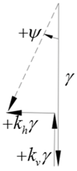
4. Extension of Cauchy’s First Law of Motion to Deformable Bodies with Internal Resistance and under the Influence of Pseudo-Static Forces

Considering the above, Cauchy’s first law of motion has been extended as to include the internal resistance of continuum, $R_i$ $\left(i\in \left\{x,y,z\right\}\right)$, and, also, to treat accelerations as causes and not as effects. Equation (1), thus, becomes:

$$\begin{array}{l}\left(\frac{\partial {\sigma }_x}{\partial x}+\frac{\partial {\tau }_{yx}}{\partial y}+\frac{\partial {\tau }_{zx}}{\partial z}-R_x\right)+f_x=\rho {\ddot{u}}_x\\ \left(\frac{\partial {\tau }_{xy}}{\partial x}+\frac{\partial {\sigma }_y}{\partial y}+\frac{\partial {\tau }_{zy}}{\partial z}-R_y\right)+f_y=\rho {\ddot{u}}_y\\ \left(\frac{\partial {\tau }_{xz}}{\partial x}+\frac{\partial {\tau }_{yz}}{\partial y}+\frac{\partial {\sigma }_z}{\partial z}-R_z\right)+f_z=\rho {\ddot{u}}_z\end{array}\},$$

(2)

where $R_i$ is the internal resistance, $f_i$ the body force and ${\ddot{u}}_{s,i}$ the imposed seismic force per unit mass in the $i$-th direction $\left(i\in \left\{x,y,z\right\}\right)$, whilst $\rho$ is the density of the material.

Intuitively, the internal resistance is given as

$$R_i=\frac{n}{z}{\tau }_{R,m},$$

(3)

where $n$ is the number of planes of the material element resisting to deformation (and thus, to the transmission of stress) and ${\tau }_{R,m}$ is the mobilized shear strength of soil. The cubic material element of Figure 1 with planes perpendicular to the coordinate axes of Cartesian coordinate system is assumed.

In Mohr–Coulomb terms the shear strength at depth $z$ is

$${\tau }_{R,m}=c_m+\gamma z\tan {\phi }_m.$$

(4)

If no shear is assumed to take place in the vertical direction, $R_z$ in Equation (2) is set to zero. This is a rational assumption especially when loads are distributed uniformly in a semi-infinite mass (as in the case of the self-weight of a material with horizontal surface and/or seismic loading), causing no relative movement of soil particles in the vertical direction.

Regarding the acceleration term, the pseudo-static concept of analysis is adopted and the imposed seismic force per unit mass will be [30]

$${\ddot{u}}_{s,i}=k_{i}g,$$

(5)

where $k_i$ is the seismic coefficient in the x, y, or z direction (usually, $k_x=k_y=k_h$ and $k_z=k_v$) and $g$ is the acceleration of gravity. The seismic coefficients may take negative values indicating the change in direction of the seismic force during an earthquake.

In geotechnical engineering gravity is usually the only body force, thus, when body forces are considered in the analysis, $f_z$ equals $\rho g$, whilst $f_x=f_y=0$.

Based on the above and replacing $\rho g$ with $\gamma$ and, also, considering the downward direction of forces as positive, Equation (2) becomes:

$$\begin{array}{l}\frac{\partial {\sigma }_x}{\partial x}+\frac{\partial {\tau }_{yx}}{\partial y}+\frac{\partial {\tau }_{zx}}{\partial z}-\frac{n}{z}\left(c_m+\left(1-k_v\right)\gamma z\tan {\phi }_m\right)=-k_h\gamma \\ \frac{\partial {\tau }_{xy}}{\partial x}+\frac{\partial {\sigma }_y}{\partial y}+\frac{\partial {\tau }_{zy}}{\partial z}-\frac{n}{z}\left(c_m+\left(1-k_v\right)\gamma z\tan {\phi }_m\right)=-k_h\gamma \\ \frac{\partial {\tau }_{xz}}{\partial x}+\frac{\partial {\tau }_{yz}}{\partial y}+\frac{\partial {\sigma }_z}{\partial z}-\gamma =-k_v\gamma \end{array}\},$$

(6)

whilst, in plane strain conditions it simplifies to:

$$\frac{\partial {\sigma }_x}{\partial x}+\frac{\partial {\tau }_{zx}}{\partial z}-\frac{2}{z}\left(c_m+\left(1-k_v\right)\gamma z\tan {\phi }_m\right)=-k_h\gamma$$

(7a)

$$\frac{\partial {\tau }_{xz}}{\partial x}+\frac{\partial {\sigma }_z}{\partial z}=\left(1-k_v\right)\gamma$$

(7b)

5. Derivation of the Proposed Generalized Coefficient of Earth Pressure at Rest

Jaky [11] considered a heap of loosely deposited sand which attains the shape of a solid of an equilateral triangle of infinite length. The slope of this loose heap of sand is assumed to be equal to the angle of internal friction (Figure 3). Jaky [11] argued that the lateral pressure acting on a line passing through the apex of the cone and is perpendicular to the base, is the lateral pressure at rest. He then divided the sand mass into two zones; a zone containing slide planes (Zone I) and the transitional zone (Zone II).

The main assumption involved in Jaky’s solution for $K_o$ is related to the distribution of shear stresses in Zone II, where, Jaky [11] assumed a parabolic distribution; this is further discussed later.

In the present problem, Jaky’s soil heap of Figure 3 is adopted but with the difference that Zone II consists of a general $c^{\prime }-{\phi }^{\prime }$ material, which has not been subjected to overstress. Zone I still consists of a purely frictional material (e.g., sand), also not overstressed (that is, it is normally consolidated). For practical purposes, the two materials have the same effective friction angle value, so that the principle trajectories remain the same. Thus, the last principle trajectory still coincides with the plane OB. In Figure 3, the slide planes have been drawn on the left-hand side of the drawing, whilst the principle stress trajectories on the right side of it.

The formulations which are based on the proposed extension of Cauchy’s first law of motion are presented in detail in Appendix A. Dividing the derived expression for ${\sigma }_{x,o}$ with the respective one for ${\sigma }_{z,o}$ (see Appendix A), the following general expression for the coefficient of lateral earth pressure is obtained

$$\begin{array}{cc}\hfill K_{xe}^{c-\phi }& =\frac{1-\sin {\phi }^{\prime }}{1+\sin {\phi }^{\prime }}\left(\left(1-\xi \sin {\phi }^{\prime }\right)+\frac{k_h}{1-k_v}\tan {\phi }^{\prime }\left(2+\xi \left(1-\sin {\phi }^{\prime }\right)\right)\right)\hfill \\ & -\frac{1}{1-k_v}\frac{2c_m}{\gamma z}\tan \left({45}^o-\frac{{\phi }^{\prime }}{2}\right)\hfill \end{array},$$

(8)

with

$$\xi =\frac{m-1}{m+1}f\left(m\right)-1,$$

(9)

and

$${\sigma }_x=K_{xe}^{c-\phi }\left(1-k_v\right)\gamma z.$$

(10)

For the derivation of Equation (7b), the author assumed a variation of shear stress in Zone II in the form:

$${\tau }_{xz}=f\left(m\right)\cdot {\tau }_{xz,OB}{\left(\frac{x}{x_{OB}}\right)}^m,$$

(11)

with

$$f\left(m\right)=1-\frac{1}{m},$$

(12)

and $(1\le m\le \infty )$. The rationality of Equation (11) and the role of the function $f(m)$ is further discussed in Section 7 and Section 10.1. Equation (8) follows the sign convention given in Appendix B.

6. The Derived Coefficients of Earth Pressures

The coefficient of earth pressure at rest will be obtained after selecting the proper value for $m$ and defining the mobilized cohesion, $c_m$. For selecting the proper $m$, the reasoning is as follows. Jaky’s [11] assumed arbitrarily the following parabolic distribution

$${\tau }_{xz}={\tau }_{xz,OB}{\left(\frac{x}{x_{OB}}\right)}^2,$$

(13)

resulting in

$$K_o=\frac{1+\frac{2}{3}\sin {\phi }^{\prime }}{1+\sin {\phi }^{\prime }}\left(1-\sin {\phi }^{\prime }\right).$$

(14)

Apparently, during his “heroic” effort in 1944 with no electronic means, Jaky must have tried the simpler and more rational linear distribution

$${\tau }_{xz}={\tau }_{xz,OB}\left(\frac{x}{x_{OB}}\right).$$

(15)

Besides, the distribution of shear stresses in Zone I follows a linear pattern (see Equation (11) in Appendix A); this distribution, however, gives singularity leading to $K_o=1$ (independently of ${\phi }^{\prime }$ value), which is not the point for sand heaps. On the other hand, from the purely theoretical point of view, the very simple $1-\sin {\phi }^{\prime }$ formula, works ideally for the two extreme values of ${\phi }^{\prime }$, where for ${\phi }^{\prime }$= 0^o it gives $K_o=1$ referring to hydrostatic conditions and for ${\phi }^{\prime }$= 90^o it gives $K_o=0$ referring to a frictional material that can stand vertically without support, thus, exerting no lateral pressure. These extreme cases are enough evidence that the correct expression for the coefficient of earth pressure at rest is the $K_o=1-\sin {\phi }^{\prime }$.

Thus, for $m=1$ (corresponding to linear distribution of shear stresses in Zone II) Equation (8) gives the proposed generalized coefficient of earth pressure at rest

$$K_{oe}^{c-\phi }=\left(1-\sin {\phi }^{\prime }\right)\left(1+\frac{k_h}{1-k_v}\tan {\phi }^{\prime }\right)-\frac{1}{1-k_v}\frac{2c_m}{\gamma z}\tan \left({45}^o-\frac{{\phi }^{\prime }}{2}\right),$$

(16)

with

$${\sigma }_{\circ }=K_{oe}^{c-\phi }\left(1-k_v\right)\gamma z.$$

(17)

For $k_h=k_v=0$ (static conditions), the coefficient of earth pressure at rest simplifies to

$$K_{oe}^{c-\phi }=\left(1-\sin {\phi }^{\prime }\right)-\frac{2c_m}{\gamma z}\tan \left({45}^o-\frac{{\phi }^{\prime }}{2}\right).$$

(18)

For $m\to \infty$, it is $\underset{m\to \infty }{\lim }\frac{m-1}{m+1}=1$ and $\underset{m\to \infty }{\lim }\frac{m+\sin {\phi }^{\prime }}{m+1}=1$, thus, the generalized coefficient of active earth pressure is obtained:

$$K_{ae}^{c-\phi }=\frac{1-\sin {\phi }^{\prime }}{1+\sin {\phi }^{\prime }}\left(1+2\frac{k_h}{1-k_v}\tan {\phi }^{\prime }\right)-\frac{1}{1-k_v}\frac{2c_m}{\gamma z}\tan \left({45}^o-\frac{{\phi }^{\prime }}{2}\right),$$

(19)

with

$${\sigma }_{\alpha }=K_{\alpha e}^{c-\phi }\left(1-k_v\right)\gamma z.$$

(20)

Additionally, if $k_h=k_v=0$, it is $c_m=c^{\prime }$ (see Section 8.2). Thus,

$$K_{ae}^{c-\phi }=\frac{1-\sin {\phi }^{\prime }}{1+\sin {\phi }^{\prime }}-\frac{2c^{\prime }}{\gamma z}\tan \left({45}^o-\frac{{\phi }^{\prime }}{2}\right),$$

(21)

with

$${\sigma }_{\alpha }=K_{ae}^{c-\phi }\gamma z=\frac{1-\sin {\phi }^{\prime }}{1+\sin {\phi }^{\prime }}\gamma z-2c^{\prime }\tan \left({45}^o-\frac{{\phi }^{\prime }}{2}\right),$$

(22)

that is, Bell’s [4] solution for the active state. Apparently, this is a compelling evidence for the validity of Equation (8) (and of course, Equation (7a)).

$K_{pe}^{c-\phi }$ can be obtained indirectly by inverting the signs of shear strength parameters in Equation (19) and that, due to the “symmetry” between the active and the passive earth pressure coefficient in the case of smooth, not battered walls retaining soil with zero backslope angle (that is, Rankine’s conditions where $\theta ={45}^o+{\phi }^{\prime }/2$ or ${45}^o-{\phi }^{\prime }/2$ for the active and the passive state, respectively). The passive earth pressure coefficient, therefore, is:

$$K_{pe}^{c-\phi }=\frac{1+\sin {\phi }^{\prime }}{1-\sin {\phi }^{\prime }}\left(1-2\frac{k_h}{1-k_v}\tan {\phi }^{\prime }\right)+\frac{1}{1-k_v}\frac{2c_m}{\gamma z}\tan \left({45}^o+\frac{{\phi }^{\prime }}{2}\right),$$

(23)

with

$${\sigma }_p=K_{pe}^{c-\phi }\left(1-k_v\right)\gamma z.$$

(24)

As in the case of the active state, if $k_h=k_v=0$, the mobilized cohesion is equal to its peak value (i.e., $c_m=c^{\prime }$; see Section 8.2). Therefore:

$$K_p^{c-\phi }=\frac{1+\sin {\phi }^{\prime }}{1-\sin {\phi }^{\prime }}+\frac{2c^{\prime }}{\gamma z}\tan \left({45}^o+\frac{{\phi }^{\prime }}{2}\right),$$

(25)

with

$${\sigma }_p=K_{pe}^{c-\phi }\gamma z=\frac{1+\sin {\phi }^{\prime }}{1-\sin {\phi }^{\prime }}\gamma z+2c^{\prime }\tan \left({45}^o+\frac{{\phi }^{\prime }}{2}\right),$$

(26)

that is, Bell’s [4] solution for the passive state.

A very interesting observation is that the number “2” in front of the cohesion term in Equations (22) and (26) is the same number appearing in author’s extension of Cauchy’s law mentioned above (recall Equation (7a)) indicating the two horizontal planes of the cubic elementary element resisting to shear in plane strain conditions, i.e., the upper and the lower face of the cubic volume element. It is reminded that Bell [4] came across the $2c^{\prime }\sqrt{K_{\alpha }}$ and $2c^{\prime }\sqrt{K_p}$ terms working fully geometrically with Mohr’s circles and Coulomb’s failure criterion. It is further noted that Bell’s solution is not able to provide explanation for the physical meaning of this numerical coefficient.

7. The “Intermediate” State of Earth Pressure

Often the wall does not translate or rotate enough so that the active or passive state can be fully mobilized. Thus, the pressure near the base is larger than predicted by theory. These pressures of intermediate state could be calculated using Equation (8) along with the proper m value.

It is noted that for $m=1$ and $\infty$, Equation (8) leads to the coefficients of earth pressure for the state at rest and the active state respectively given earlier. In addition, due to the known “symmetry” between the active and the passive earth pressure coefficient, Equation (8) can be written in the following form:

$$\begin{array}{cc}\hfill K_{xe}^{c-\phi }& =\left\{\begin{array}{l}\mathrm{active}“\mathrm{side}”;\\ \mathrm{from}{K}_{oe}^{c-\phi }(m=1)\mathrm{to}{K}_{ae}^{c-\phi }(m=+\infty );{\xi }_1={\xi }_2=1\\ \mathrm{passive}“\mathrm{side}”;\\ \mathrm{from}{K}_{oe}^{c-\phi }(m=1)\mathrm{to}{K}_{pe}^{c-\phi }(m=+\infty );{\xi }_1=1+\xi ;{\xi }_2=\frac{2}{m}-1\end{array}\right\}\hfill \\ & ={\left(\frac{1\mp \sin {\phi }^{\prime }}{1\pm \sin {\phi }^{\prime }}\right)}^{{\xi }_1}\left(\left(1\mp \xi \sin {\phi }^{\prime }\right)\mp {\xi }_2\frac{k_h}{1-k_v}\tan {\phi }^{\prime }\left(2+\xi \left(1\mp \sin {\phi }^{\prime }\right)\right)\right)\hfill \\ & \mp \frac{1}{1-k_v}\frac{2c_m}{\gamma z}{\left(\frac{\tan \left({45}^o\mp \frac{{\phi }^{\prime }}{2}\right)}{\tan \left({45}^o\pm \frac{{\phi }^{\prime }}{2}\right)}\right)}^{{\xi }_1}\tan \left({45}^o\pm \frac{{\phi }^{\prime }}{2}\right)\hfill \end{array},$$

(27)

where, ${\xi }_1$ and ${\xi }_2$ are parameters related to the transition from the soil wedge of the state at rest to the soil wedge of the passive state (i.e., inclination angle of soil wedge changing from 45 + ${\phi }^{\prime }/2$ to 45- ${\phi }^{\prime }/2$). $m$ is always positive meaning that, for the passive “side” $m$ ranges between 1 (state at rest) and $+\infty$ (passive state). The symmetry stands for smooth, not battered wall with zero backslope angle.

For any m value between these extremes (i.e., 1 and $+\infty$), Equation (27) gives the coefficient of earth pressure at rest; however, m must be defined with respect to the wall movement. In this respect, Finn [31] gave analytical expressions for the pressure behind smooth and rough translating wall which moves outwards at a distance $\Delta x$. He also gave expressions for the case of rotating wall as for the top. According to Finn, the lateral earth pressure at depth $z$ on a smooth wall that has been displaced laterally by $\Delta x$ is:

$${\sigma }_{h,Finn}=\frac{\mu }{1-\mu }\gamma z-\frac{E_{Young}}{\left(1-{\mu }^2\right)\pi }\frac{4H^{2}z}{{\left(z+H\right)}^3\left(H-z\right)}\Delta x,$$

(28)

for smooth translating wall and

$$\begin{array}{cc}\hfill {\sigma }_{h,Finn}& =\frac{\mu }{1-\mu }\gamma z-\frac{4E_{Young}H}{\pi \left(3-\mu -4{\mu }^2\right)\left(1+\mu \right)}·\hfill \\ & ·\left(\frac{1-{\mu }^2}{H^2-z^2}+\frac{\mu \left(1+\mu \right)H-\left(1-{\mu }^2\right)z}{{\left(H+z\right)}^3}\right)\Delta x\hfill \end{array},$$

(29)

for rough translating wall.

Note: “Equation 107” in Finn [31] for ${\sigma }_{h,Finn}$ for the case of rough translating wall has a typographical error. This error has been corrected in Equation (29). Additionally, some signs in Equation (29) have been inverted because herein $\Delta x$ is always positive quantity; in Finn [31], when the wall moves away of soil, this distance in considered negative.

Re-evaluating the above expression, the procedure for the active case will have as follows: first, ${\sigma }_{h,Finn}$ is replaced by Equation (10) and the term $(\mu /(1-\mu ))\gamma z$ (representing the static earth pressure at rest in $\mu$ terms) by Equation (16); then, solving as for $\Delta x$, the required displacement for the active state to fully develop at depth $z$ will be:

$$\Delta x_{\max }=\frac{\pi }{4}\frac{\left(1-{\mu }^2\right)}{E_{Young}}\frac{{\left(H+z\right)}^3\left(H-z\right)}{H^{2}z}\Delta K\left(1-k_v\right)\gamma z,$$

(30)

for smooth translating wall and

$$\begin{array}{cc}\hfill \Delta x_{\max }& =\frac{\pi }{4}\frac{\left(3-\mu -4{\mu }^2\right)\left(1+\mu \right)}{E_{Young}}·\hfill \\ & ·{\left(\frac{1-{\mu }^2}{H^2-z^2}+\frac{\mu \left(1+\mu \right)H-\left(1-{\mu }^2\right)z}{{\left(H+z\right)}^3}\right)}^{-1}\cdot \frac{1}{H}\Delta K\left(1-k_v\right)\gamma z\hfill \end{array},$$

(31)

for rough translating wall. $\Delta K=K_{oe}^{c-\phi }-K_{xe}^{c-\phi }$ or $K_{xe}^{c-\phi }-K_{oe}^{c-\phi }$ (depending on the case).

Assuming a linear relationship between $f(m)=1-1/m$ and $\Delta x/\Delta x_{\max }$, $m$ is given by the following equation:

$$m={\left(1-\frac{\Delta x}{\Delta x_{\max }}\right)}^{-1}\left\{0\le \Delta x\le \Delta x_{\max };\mathrm{if}\Delta x>\Delta x_{\max },m=\infty \right\}.$$

(32)

The rationality of the latter is discussed in the “application examples” section.

8. The Mobilized Shear Strength of Soil

An essential part of the present solution is the calculation of the mobilized shear strength of soil. For $c^{\prime }-{\phi }^{\prime }$ materials the rational assumption that cohesion and friction are mobilized in equal proportions is made, that is,

$$\tan {\phi }_m=\frac{\tan {\phi }^{\prime }}{f_m},$$

(33)

and

$$c_m=\frac{c^{\prime }}{f_m}.$$

(34)

The above assumption reminds of the traditional safety factor defined with respect to shear strength in Mohr–Coulomb terms (see [32,33]).

8.1. The Mobilized Shear Strength of Soil in the State at Rest

Schematically, the tangent to Mohr circle representing the state at rest at a specific depth, crosses the axis of normal stresses at distance $c_m/\tan {\phi }_m$ to the left of the point of origin (distance $(AO)$ in Figure 4). Substituting $c_m$ and $\tan {\phi }_m$ from above, $(AO)=c^{\prime }/\tan \phi$. The same distance is obtained for both the active and passive state under static conditions, where, in this respect, the tangent to the circle is the Mohr–Coulomb’s failure criterion. From the above it is inferred that the point A in Figure 4 is also the pivot point for any intermediate state between the active and the passive one, including, of course, the state at rest.

Geometrically, from Figure 4, the mobilized friction angle is given by the following equation:

$$\sin {\phi }_m=\frac{\pm \left(\frac{\left(1-k_v\right)\gamma z-K_{oe}^{c-\phi }\left(1-k_v\right)\gamma z}{2}\right)}{\frac{c^{\prime }}{\tan {\phi }^{\prime }}+\frac{\left(1-k_v\right)\gamma z+K_{oe}^{c-\phi }\left(1-k_v\right)\gamma z}{2}}.$$

(35)

The plus sign, in the equation above, stands for the usual case that $K_{oe}^{c-\phi }<1$. It is assumed that an extreme earthquake event in combination with a weak material may cause $K_{oe}^{c-\phi }$ to exceed unity. In such a case, the minus symbol is used.

Substituting Equation (16) into Equation (35) with the $2c_m/\gamma z$ term inside $K_{oe}^{c-\phi }$, to have been replaced with $2c^{\prime }/\left(\gamma z{f}_m\right)$, with the use of Equation (34)

$$\sin {\phi }_m=\frac{\pm \left(e_1+\frac{1}{f_m}\right)}{e_2-\frac{1}{f_m}},$$

(36)

with

$$e_1=\frac{\left(1-k_v\right)\left(1-\left(1-\sin {\phi }^{\prime }\right)\left(1+\frac{k_h}{1-k_v}\tan {\phi }^{\prime }\right)\right)}{\frac{2c^{\prime }}{\gamma z}\tan \left({45}^{\circ }-\frac{{\phi }^{\prime }}{2}\right)}.$$

(37)

$$e_2=\frac{\tan \left({45}^{\circ }+\frac{{\phi }^{\prime }}{2}\right)}{\tan {\phi }^{\prime }}+\frac{\left(1-k_v\right)\left(1+\left(1-\sin {\phi }^{\prime }\right)\left(1+\frac{k_h}{1-k_v}\tan {\phi }^{\prime }\right)\right)}{\frac{2c^{\prime }}{\gamma z}\tan \left({45}^{\circ }-\frac{{\phi }^{\prime }}{2}\right)},$$

(38)

and

$$\frac{1}{f_m}=\frac{\tan {\phi }_m}{\tan {\phi }^{\prime }}.$$

(39)

The analytical solution of Equation (36) is given in the Appendix C.

8.2. The Mobilized Shear Strength of Soil in the Active and Passive State

As known, the mobilized shear strength of soils under static conditions is equal to the peak strength. However, only part of the shear strength of soil is mobilized under dynamic conditions. For example, in the active state it stands that $K_{ae}>K_a$. Thus, a Mohr circle representing the active state of stress under dynamic conditions with ${\sigma }_3=K_{ae}\gamma z\left(1-k_v\right)$ and ${\sigma }_1=\gamma z\left(1-k_v\right)$ lies inside the respective one representing static conditions with ${\sigma }_3=K_a\gamma z$ and ${\sigma }_1=\gamma z$. The latter, as known, corresponds to state of failure touching the Coulomb’s failure criterion, whilst the Mohr circle representing dynamic condition does not. The same also stands, of course, for the passive state because $K_{pe}<K_p$. In the example above, $k_v$ was considered positive; however, a negative $k_v$ does not change the general observation.

As it will be shown below, however, an earthquake excitation causes the reduction of the shear strength of soil mobilized during an earthquake event. Thus, with smaller (mobilized) shear strength, the soil exerts greater earth pressure on the retaining structure. The amount of the resisting forces (or moments) in relation to the destabilizing forces (or moments) defines, finally, whether the earth retaining structure will be stable or not. If the retaining structure is allowed to be displaced enough so that failure occurs, the Rankine’s theory will give again the minimum or maximum earth pressure in the active and passive state, respectively.

For the active and passive state, the mobilized shear strength is calculated following the steps described for the state at rest. In this respect, geometrically, from Figure 4 (after replacing $K_{oe}^{c-\phi }$ with $K_{ae}^{c-\phi }$), the mobilized friction angle for the active state is given by the following equation:

$$\sin {\phi }_m=\frac{\pm \left(\frac{\left(1-k_v\right)\gamma z-K_{\alpha e}^{c-\phi }\left(1-k_v\right)\gamma z}{2}\right)}{\frac{c^{\prime }}{\tan {\phi }^{\prime }}+\frac{\left(1-k_v\right)\gamma z+K_{\alpha e}^{c-\phi }\left(1-k_v\right)\gamma z}{2}}.$$

(40)

The plus sign, in the equation above, stands for the more probable case where $K_{\alpha e}^{c-\phi }<1$, although, an extreme earthquake event in combination with a weak soil could cause $K_{\alpha e}^{c-\phi }$ to exceed unity. A parametric study carried out by the author, however, showed that precondition for this unusual case to occur is that the shear strength of soil is very small and simultaneously that the seismic event is rather unrealistically extreme. Thus, since this condition is rather impossible to occur in practice, it is not further discussed here.

By substituting Equation (19) into Equation (40) with the term $2c_m/\gamma z$ inside $K_{\alpha e}^{c-\phi }$ to have been replaced by the term $2c^{\prime }/\left(\gamma z{f}_m\right)$ (recall Equation (34)), Equation (36) is again obtained, but with

$$e_1=\frac{\left(1-k_v\right)\left(1-\frac{1-\sin {\phi }^{\prime }}{1+\sin {\phi }^{\prime }}\left(1+2\frac{k_h}{1-k_v}\tan {\phi }^{\prime }\right)\right)}{\frac{2c^{\prime }}{\gamma z}\tan \left({45}^{\circ }-\frac{{\phi }^{\prime }}{2}\right)},$$

(41)

and

$$e_2=\frac{\tan \left({45}^{\circ }+\frac{{\phi }^{\prime }}{2}\right)}{\tan {\phi }^{\prime }}+\frac{\left(1-k_v\right)\left(1+\frac{1-\sin {\phi }^{\prime }}{1+\sin {\phi }^{\prime }}\left(1+2\frac{k_h}{1-k_v}\tan {\phi }^{\prime }\right)\right)}{\frac{2c^{\prime }}{\gamma z}\tan \left({45}^{\circ }-\frac{{\phi }^{\prime }}{2}\right)}.$$

(42)

In a similar way, the $e_1$ and $e_2$ parameters for the passive state are

$$e_1=-\left(\frac{\left(1-k_v\right)\left(1-\frac{1+\sin {\phi }^{\prime }}{1-\sin {\phi }^{\prime }}\left(1-2\frac{k_h}{1-k_v}\tan {\phi }^{\prime }\right)\right)}{\frac{2c^{\prime }}{\gamma z}\tan \left({45}^{\circ }+\frac{{\phi }^{\prime }}{2}\right)}\right),$$

(43)

$$e_2=-\left(\frac{\tan \left({45}^{\circ }-\frac{{\phi }^{\prime }}{2}\right)}{\tan {\phi }^{\prime }}+\frac{\left(1-k_v\right)\left(1+\frac{1+\sin {\phi }^{\prime }}{1-\sin {\phi }^{\prime }}\left(1-2\frac{k_h}{1-k_v}\tan {\phi }^{\prime }\right)\right)}{\frac{2c^{\prime }}{\gamma z}\tan \left({45}^{\circ }+\frac{{\phi }^{\prime }}{2}\right)}\right).$$

(44)

8.3. The Mobilized Shear Strength of Soil in the Intermediate State

For the intermediate state of earth pressures on the active side the parameters e₁ and e₂ are given below:

$$e_1=\frac{\left(1-k_v\right)\left(1-\frac{1-\sin {\phi }^{\prime }}{1+\sin {\phi }^{\prime }}\left(\left(1-\xi \sin {\phi }^{\prime }\right)-\frac{k_h}{1-k_v}\tan {\phi }^{\prime }\left(2+\xi \left(1-\sin {\phi }^{\prime }\right)\right)\right)\right)}{2\frac{c^{\prime }}{\gamma z}B},$$

(45)

$$\begin{array}{l}{e}_2=\frac{\tan \left({45}^o+\frac{{\phi }^{\prime }}{2}\right)}{\tan {\phi }^{\prime }}+\\ \frac{\left(1-k_v\right)\left(1+\frac{1-\sin {\phi }^{\prime }}{1+\sin {\phi }^{\prime }}\left(\left(1-\xi \sin {\phi }^{\prime }\right)-\frac{k_h}{1-k_v}\tan {\phi }^{\prime }\left(2+\xi \left(1-\sin {\phi }^{\prime }\right)\right)\right)\right)}{\frac{2c^{\prime }}{\gamma z}\tan \left({45}^o-\frac{{\phi }^{\prime }}{2}\right)}\end{array}$$

(46)

For the intermediate state on the passive side the parameters e₁ and e₂ are given in the Appendix D. Moreover, it is noted that, $\lambda =1$ and 0 for pressures on the active and passive “side”, respectively. For the active state or “side”, the author suggests that the calculation of earth pressures be restricted to the positive values. Otherwise, the value $\lambda =2$ may be needed near the top of the wall where the earth pressures are negative due to cohesion; the continuity of the distribution will show when the $\lambda$=2 value is required to be used.

9. Depth of Neutral Zone (State at Rest) and Tension Crack (Active State)

9.1. Depth of Neutral Zone (State at Rest)

Apparently, the presence of cohesion creates a neutral zone extending to depth $z_{nz}$ from the surface. In this neutral zone no lateral earth pressure is exerted. The depth of this zone can be obtained from Equation (35) setting $K_{\circ e}^{c-\phi }=0$ and solving as for $z$, where:

$$z_{nz}=\frac{2c^{\prime }}{\left(1-k_v\right)\gamma }\frac{\sin {\phi }_m}{\left(1-\sin {\phi }_m\right)\tan {\phi }^{\prime }}.$$

(47)

By further processing Equation (47) along with Equation (16) $(K_{\circ e}^{c-\phi })$ and the necessary trigonometric identities, the depth of neutral zone is

$$z_{nz}=\frac{c^{\prime }}{(1-k_v)\gamma \tan {\phi }^{\prime }}\left[\frac{1}{{\left(\cos {\phi }^{\prime }+\frac{k_h}{1-k_v}\sin {\phi }^{\prime }\right)}^2}-1\right].$$

(48)

From Equation (48) it is inferred that a neutral zone exists, apparently in cohesive materials, but only when

$$\frac{k_h}{1-k_v}<\frac{1-\cos {\phi }^{\prime }}{\sin {\phi }^{\prime }}.$$

(49)

9.2. Depth of Tension Crack (Active State)

The depth of tension crack can be taken from Equation (40) by setting $K_{ae}^{c-\phi }=0$ and solving as for $z$, where:

$$z_{tc}=\frac{2c^{\prime }}{\left(1-k_v\right)\gamma }\frac{\sin {\phi }_m}{\left(1-\sin {\phi }_m\right)\tan {\phi }^{\prime }}.$$

(50)

By further processing Equation (50) along with Equation (19) for $K_{ae}^{c-\phi }$ and the necessary trigonometric identities, the following more convenient expression for the depth of tension crack is obtained:

$$z_{tc}=\frac{c^{\prime }}{(1-k_v)\gamma \tan {\phi }^{\prime }}\left[\frac{{\tan }^2\left({45}^o+\frac{{\phi }^{\prime }}{2}\right)}{{\left(1+2\frac{k_h}{1-k_v}\tan {\phi }^{\prime }\right)}^2}-1\right].$$

(51)

From Equation (51) it is inferred that cohesion is not the only precondition for the development of tension crack. In addition, the following condition should be satisfied:

$$\frac{k_h}{1-k_v}<\frac{\tan \left({45}^o+\frac{{\phi }^{\prime }}{2}\right)-1}{2\tan {\phi }^{\prime }}.$$

(52)

For static conditions ($k_h=k_v=0$) it stands that $c_m=c^{\prime }$ (based on Section 8.2), thus, Equation (51) simplifies to the well-known

$$z_{tc}=\frac{2c^{\prime }}{\gamma \tan \left({45}^o-\frac{{\phi }^{\prime }}{2}\right)}.$$

(53)

10. Discussion

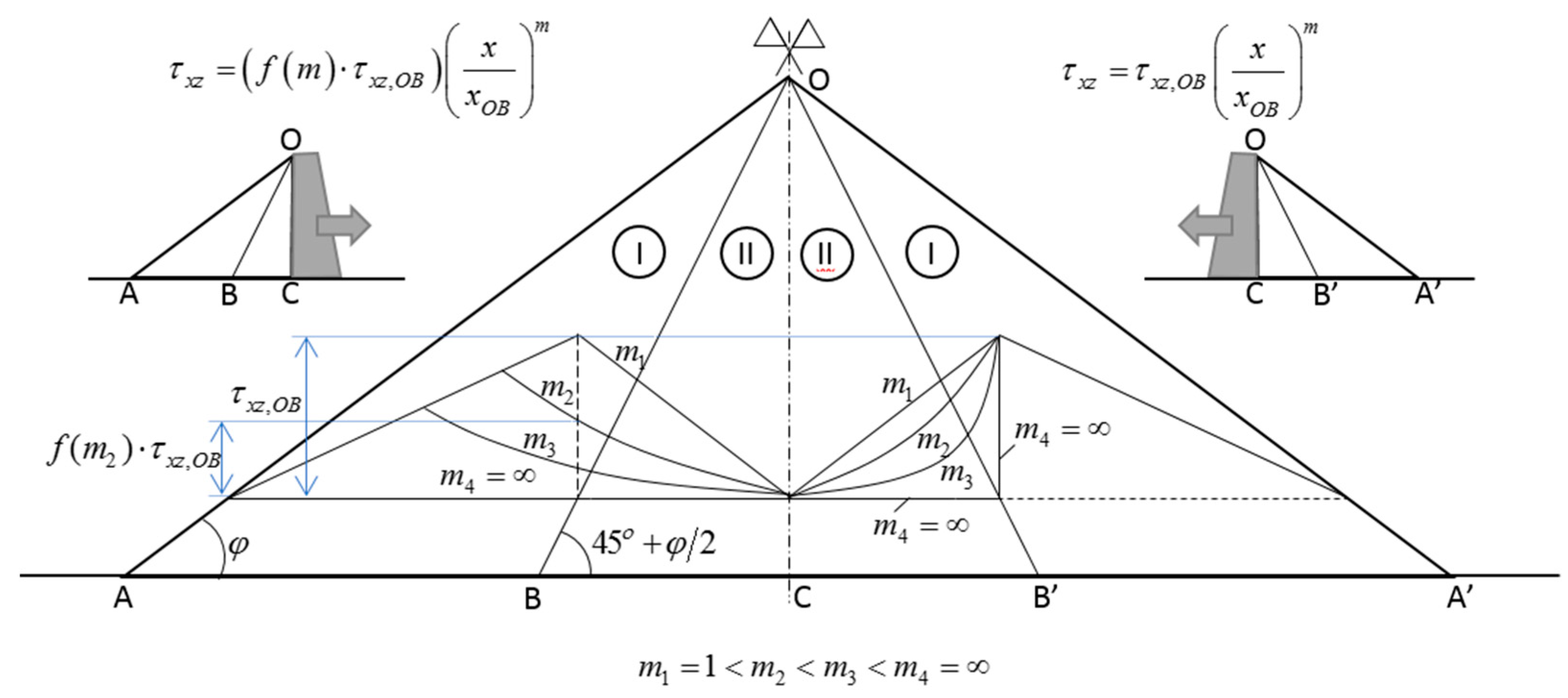
10.1. Choosing a Rational f(m) Function

The use of the $f(m)$ function (recall Equation (11)) in Equation (12) is deemed necessary because a variation of shear stress in the form of:

$${\tau }_{xz}={\tau }_{xz,OB}{\left(\frac{x}{x_{OB}}\right)}^m,$$

(54)

leads to unrealistic stress components in Zone II [34,35]. The problematic behavior of Equation (54) is better interpreted considering that the one of the two halves of the symmetrical sand heap has been replaced by a rigid retaining wall which is translating away from the other half (half sand heap) until the latter to reach the active state (see Figure 5). During this translational movement, the outer zone of the sand heap (Zone I) gradually fails as it gradually loses its support; in this respect, the failure of the inner zone (Zone II, zone between line OB and OC in Figure 5) precedes. Thus, the shear stress ${\tau }_{xz}$ on OB is not constant and equal to ${\tau }_{xz,OB}$ but a portion of ${\tau }_{xz,OB}$ which becomes lower and lower as the soil heap fails, i.e., ${\tau }_{xz}=f(m)\cdot {\tau }_{xz,OB}$; $f(m)$ ranges between 1 and 0 for the state at rest and the active state respectively.

$f\left(m\right)$ could have the following more generalized form:

$$f\left(m\right)=1-\frac{a}{m}.$$

(55)

However, if $a>1$, for values of $m$ close to unity Equation (55) leads to intermediate earth pressures (on the active side) greater than the respective earth pressures at rest; something that is not admissible. For any $0<a<1$ Equation (55) gives intermediate earth pressures less conservative as compared to those obtained from Equation (12). Thus, Equation (12) seems to be the best choice for the function $f\left(m\right)$.

The two assumed shear stress functions given by Equations (11) and (54) are compared through the coefficient $K_{xe}^{c-\phi }$. The data used were $c^{\prime }=$ 0 or 20 kPa, ${\phi }^{\prime }={30}^{\circ }$, $\gamma =18kN/m^3$, $k_h=0.3$, and $k_v=k_h/2$. As it is shown in Figure 6, Equation (11) is not only more rational (as explained above), but also gives more conservative results as compared to Equation (54).

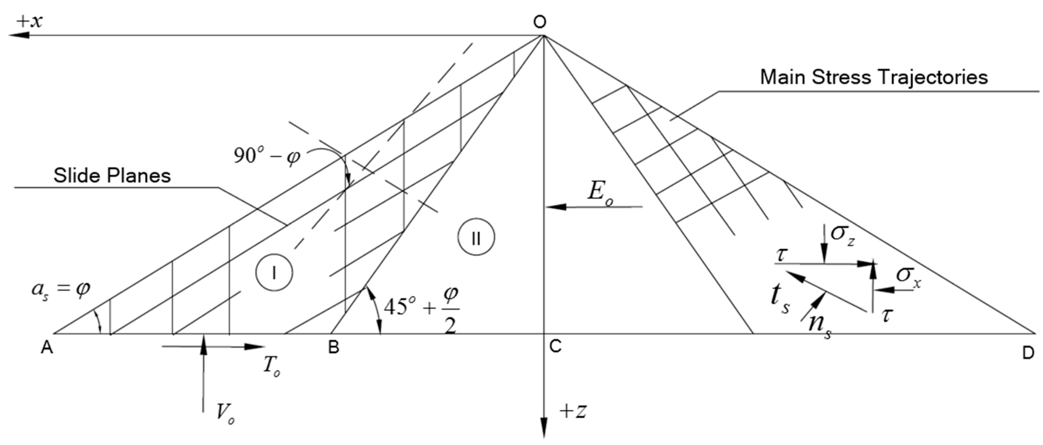
10.2. Validity of Sand Heap Hypothesis

Michalowski [34] and Pipatpongsa and Vardhanabhuti [35] infer that Jaky’s [11] derivation of $K_o$ is coincidental because the resulting stress distributions in Zone II look unrealistic due to the appearance of a local minimum. Although the appearance of unrealistic local minimum is generally true, there are two cases that the generalized parabola of Equation (54) (controlled by the empirical exponent $m$) leads to admissible stress distributions. More specifically, for $m\to 1$ the shear stress distribution becomes linear corresponding to the state at rest, whilst for $m\to \infty$ the shear stress nullifies inside the core of sand heap (Zone II) corresponding to the active state of failure; that is, for $0\le x/x_{OB}\le 1$, the ${(x/x_{OB})}^{\infty }$ term in Equation (54) tends to zero and thus, the shear stress ${\tau }_{xz}$ becomes equal to zero. The validity of the linear distribution (for $m\to 1$) was discussed in Section 6. On the other hand, the validity of the $m\to \infty$ case is strongly supported by the fact that the proposed continuum mechanics approach under static conditions leads to Bell’s solution for the active earth pressure for $c^{\prime }-{\phi }^{\prime }$ soils (recall Equation (22)).

Let us now consider that the half (symmetrical) sand heap is retained by a smooth vertical wall. Since the $m\to 1$ value corresponds to the state at rest (stable condition) and the $m\to \infty$ value to the active state of failure (unstable condition), by increasing the $m$ value from 1 to $\infty$, failure is gradually provoked to the core of the sand heap (Zone II). The crust of sand heap (Zone I), as it loses its support, will also fail, following the collapse of Zone II. Thus, both Michalowski [34] and Pipatpongsa and Vardhanabhuti [35] in their stress distribution representations in the soil heap considered erroneously together an unstable zone (Zone II; core of sand heap) with a stable one (Zone I; crust of sand heap), which normally should not be stable. In other words, the so-called “unreliable local minimum” is observed because the parabola of the vertical stresses in Zone II “dives” to reach a minimum value “jumping” from a value (on the boundary OB) that has erroneously been kept fixed and high (see “Figure 2c” in Michalowski [34] and “Figure 3” in Pipatpongsa and Vardhanabhuti [35]).

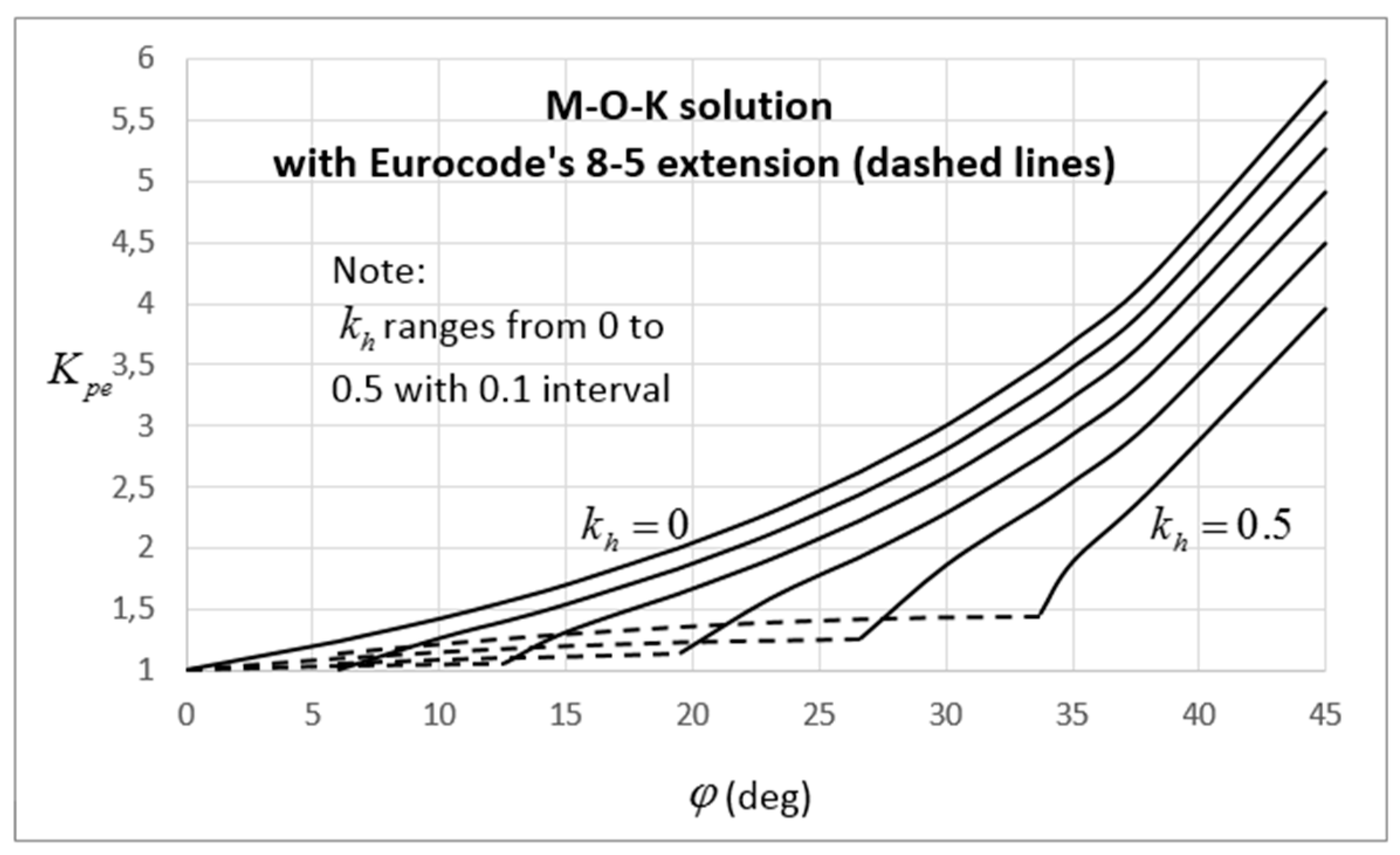
10.3. Comparison of the Proposed Coefficients with Existing Solutions and Experimental Results

The proposed coefficients will be compared with those given by Mononobe–Okabe (M-O) [7,8] and Kapila [9] (Mononobe–Okabe–Kapila or M-O-K) for the active and the passive state, respectively. These coefficients are not only the most widely used in academia and in practice, but also they are included in numerous seismic design codes worldwide (e.g., [36,37]), since being suggested as standard methods by Seed and Whitman [38].

A set of $K_{ae}$ and $K_{pe}$ versus ${\phi }^{\prime }$ curves were drawn for comparison purposes for various $k_h$ values and $k_v=k_h/2$; see Figure 7, Figure 8, Figure 9 and Figure 10 (the curves drawn are for cohesionless soils). Regarding M-O and M-O-K solutions, it is very weird that both are not applicable to all $k_h-{\phi }^{\prime }$ combinations (see Figure 8 and Figure 10). The problems with these two solutions are known (e.g., see [39]) with the most important one being the square root of negative number in Equations (56) and (57) for ${\phi }^{\prime }<\psi \mp \beta$ (the minus sign stands for the active case whilst the plus sign stands for the passive case); this issue is further discussed in Section 10.4.

$$K_{ae,M-O}=\frac{{\cos }^2\left({\phi }^{\prime }-\psi -\beta \right)}{\cos \psi {\cos }^2\beta \cos \left(\delta +\beta +\psi \right){\left(1+\sqrt{\frac{\sin \left({\phi }^{\prime }+\delta \right)\sin \left({\phi }^{\prime }-\psi -{\alpha }_s\right)}{\cos \left(\delta +\beta +\psi \right)\cos \left({\alpha }_s-\beta \right)}}\right)}^2},$$

(56)

$$K_{pe,M-O-K}=\frac{{\cos }^2\left({\phi }^{\prime }-\psi +\beta \right)}{\cos \psi {\cos }^2\beta \cos \left(\delta -\beta +\psi \right){\left(1-\sqrt{\frac{\sin \left({\phi }^{\prime }+\delta \right)\sin \left({\phi }^{\prime }-\psi +{\alpha }_s\right)}{\cos \left(\delta -\beta +\psi \right)\cos \left({\alpha }_s-\beta \right)}}\right)}^2},$$

(57)

where $\psi$ is the angle of the resultant body force in the soil from vertical (Figure 11):

$$\psi =\arctan \left(\frac{k_h}{1-k_v}\right).$$

(58)

On the other hand, the proposed solution gives smooth and continuous curves, being able to calculate the active and passive earth pressure on the wall in every case (Figure 7 and Figure 9). It is very interesting that, following the M-O-K method, a catastrophic earthquake with $k_h=0.5$ and $k_v=0.25$, seems to have a relatively minor effect on the reduction of passive resistance. On the contrary, when the proposed procedure is followed the reduction of passive resistance appears to be more rational. Indeed, negative values may be obtained under extreme seismic accelerations. In this special case of passive failure, the horizontal pressure ${\sigma }_3$ in Mohr’s diagram is not only to the left of ${\sigma }_1$ (where the circles for the active state are traditionally drawn), but also to the left of the point of origin.

Another interesting point is that, for ${\phi }^{\prime }=0^o$, the proposed coefficients of active and passive earth pressures equal unity. Actually, as shown in Figure 12, this value is the transition point between the active and the passive state. Moreover, despite the noncontinuity of the original M-O and M-O-K solutions, they are both defined for ${\phi }^{\prime }=0^o$, giving $K_{ae}$ and $K_{pe}$ values also equal to unity for any $k_h$-$k_v$ combination. Using the (arbitrary) correction given in Eurocode 8-5 [36] for the M-O and M-O-K solutions, unity is also the transition point between the active and the passive state (see dashed lines in Figure 8 and Figure 10).

From Figure 7, Figure 8, Figure 9 and Figure 10 it is also inferred that the proposed solution is less conservative for the active case and more conservative for the passive case. However, the question is not to find a solution that is more conservative, but a solution that effectively reflects reality; and this because the cost of an overconservative design can be just as much of a problem as the cost of a future failure [40]. Over the last decades, a great number of experimental, numerical, and analytical studies led to a consensus that the M-O method yields conservative earth pressure values and excessively conservative values for Peak Ground Accelerations (PGA) in excess of 0.4 g (e.g., [40,41,42,43,44,45,46,47,48,49,50,51,52,53]). Generally, these studies refer to the active state, although some of them refer to the M-O-K solution for the passive state [47,54].

Some authorities have already recognized the conservatism of the M-O solution adopting as standard design practice the use of a reduction coefficient for the expected peak ground acceleration [37,39,55,56]. For example, AASHTO [37] suggests $k_h=(1/2)PGA$, whilst the Building Seismic Safety Council [56] suggests $k_h=(2/3)PGA$; the latter has been based on the centrifuge model tests of Sitar and Al Atik [46]. Centrifuge tests have the advantage of avoiding the limitations of the 1-g shaking table, whilst scaling laws can be accurately followed. However, they also present challenges particularly when it comes to the ability of conventional instrumentation to adequately respond at frequencies dictated by the scaled model response characteristics [40]; this is further discussed in Section 10.3.

The $K_{ae}$-${\phi }^{\prime }$ relation for $k_h$ values corresponding to seismic coefficients equal to the 2/3 and 1/2 of PGA is also shown in Figure 8 (first and second values in brackets, respectively). In this respect, it is amazing how this correction brings the M-O coefficient values so close to the coefficient values derived by the proposed solution (please compare Figure 7 with Figure 8, but using the $k_h$ values given in brackets in Figure 8). The proposed solution compares also excellently to the “loma prieta sc” and “kobe tak090” centrifuge tests performed on cantilever walls by Mikola and Sitar (see “Figure 4.26” in [44]). The specific tests were chosen due to their excellent calibration as confirmed by the static earth pressure distributions (“Figure 4.22” in [44]).

Actually, the problem with both M-O and M-O-K solutions is found in the procedure followed for the derivation of the well-known coefficients of Equations (56) and (57). It is reminded that both M-O and M-O-K solutions are extensions of the well-known Coulomb’s solution for earth pressures. For the derivation to his solution under static conditions, Coulomb performed a force polygon analysis considering a rigid soil wedge defined by the inner face of the retaining wall, the backfill slope, and the rapture surface (see [57]); as the soil wedge is marginally stable, Coulomb used the peak shear strength value of soil along the rapture surface. In a similar way, Mononobe–Okabe [7,8] and Kapila [9] also treated the soil wedge as being in the state of failure using peak shear strength values. However, as mentioned in Section 8.2, the mobilized shear strength of soil should have been used. In this respect it is mentioned that the reduced $k_h$ values, i.e., $k_h=(1/2)PGA$ and $k_h=(2/3)PGA$ used by AASHTO [37] and Building Seismic Safety Council [56] compensate this error empirically.

10.4. Point of Application of the Resultant Force under Dynamic Conditions

The point of application of the resultant force under dynamic conditions is also a long-standing problem. Indeed, over the last 80 years a great number of experimental, numerical, and analytical studies have been proposed.

Probably the most widely spread works are the experimental findings of Sherif et al. [58] and Sherif and Fang [59,60], the analytical solution of Prakash and Basavanna [61], and the suggestions of Seed and Whitman [38]. Generally, all these works recommend that the point of application of the resultant force under dynamic conditions be taken (much) higher than the one-third of the height of the retained soil (measured from the lower point of the wall).

About the experimental works, it is noted that most of them have been conducted on very short walls (usually up to a meter high and often of the order of a few tens of centimeters) equipped with small earth pressure cells. In this respect, Dunnicliff [62] lists 14 “major factors affecting measurements” with embedment earth pressure cells, plus, the need for calibration (often special calibration) prior to each use. Indicatively, an example of erroneous measurements can be found in Sherif and Fang [60], where the measured active earth pressure under static conditions by the upper two (out of the six) earth pressure cells is much higher compared to the respective earth pressure at rest (please notice the weird bulge in “Figure 5” of [59]). The latter was calculated by the author with Jaky’s $K_o=1-\sin {\phi }^{\prime }$ formula, in which it is widely accepted that it performs satisfactorily in practice. It is also clear from the same figure that the same issue seriously affected Sherif and Fang’s measurements under dynamic loading. It is mentioned that Sherif and Fang’s model was 1 m in height (40-in), whilst they used diaphragm-type Kulite VM-750 soil pressure transducers (diaphragm diameter = 1.27 cm).

The author chose to present below three out of the 14 major factors mentioned by Dunnicliff [62] affecting experimental investigations; not mentioning cell calibration.

About the size of cells Dunnicliff [62] mentions that, “small cells (50–75 mm) are, generally, not recommended because scale effects and placement problems are likely to cause greater errors than for larger cells (230–300 mm)”. However, large cells, by definition, were not possible to be used in models of the order of some tens of centimeters.

The confining conditions is another major source of error (see [40,41,62,63,64,65,66]). The limited extend of laboratory models in plan and cross-section view affects the measurements due to “reflection” of stresses on the boundaries (action and reaction phenomenon). Weiler and Kulhawy [63] characteristically mention that “the boundary conditions of the chamber in which the stress cells are calibrated are very important to the stress-strain response of soil”. According to the author, probably the “confining conditions” is enough reason for the earth pressure distribution to appear bloated, affecting, in turn, the point of application.

The “dynamic stress measurements” is another important factor, with the response time, the natural frequency, and the inertia of cell being the main causes of error [40,62,63,64]. Stress cells give the best results when used in static conditions. In the case of dynamic loading, special precautions are necessary [63]. According to Weiler and Kulhawy [63], previous studies of stress cells under dynamic loadings failed to reveal any consistent pattern or behavior.

About analytical solutions, Prakash and Basavanna [61] imply that the assumption that the point of application in Mononobe–Okabe’s solution lies at $H/3$ from the bottom is not valid because the equilibrium of moments (in addition to the equilibrium of forces in the two directions) is not satisfied. Working with Coulomb’s rigid wedge, they proposed a methodology for calculating the earth pressures and the point of application of the resultant force when the equilibrium of forces ‘or’ the equilibrium of moments is satisfied. That is, in Prakash and Basavanna [61] the equilibrium of forces and moments are still not satisfied simultaneously, calculating (for the same problem) different resultant force and point of application from the equilibrium of forces and different from the equilibrium of moments. Moreover, in this work it is assumed that the shear resistance along the plane of rapture is fully mobilized. However, during dynamic solutions, as explained previously, the shear strength of soils is not fully mobilized. That means that, working with Coulomb’s rigid wedge, the resultant reaction force on the assumed failure plane inclines upward at a greater angle with respect to horizontal than the one defined by the mobilized friction angle. Indeed, this is the reason why in Prakash and Basavanna’s [61] analysis the resultant force acts much higher than the one-third of the height of the retained soil.

About the suggestion of Seed and Whitman [38] and the broadly-known distance of $0.6H$ (that is, the distance where the dynamic pressure increment $\Delta P_{AE}$ acts on the wall), it is mentioned that this was taken from a very early experimental work (published in 1939 under the title “Tennessee Valley Authority Requirements for Lateral Pressures in Earthquake Resistant Design”). Actually, this is an intermediate, rounded value of two different wall batter cases ($0.67H$ for wall batter <4:12 and $0.58H$ for wall batter >4:12). Apparently, this very early experimental work carries a lot of the disadvantages discussed herein.

Finally, it is mentioned that the most recent experimental (centrifuge tests), numerical, and analytical studies show that the distribution of dynamic earth pressure is triangular or near triangular and consequently the point of application lies at $H/3$ from the bottom or near this point (e.g., [40,41,43,44,48,50,53,65,67,68]). These studies agree with the outcomes of the present analysis.

10.5. How Design Codes Treat Dynamic Earth Pressures on Retaining Structures

As mentioned previously, the methods preferred by the various design codes for the calculation of active and passive earth pressures under seismic conditions are the M-O and M-O-K. The various design codes recognize the limitations of these methods and they either attempt an interpretation, dictate a modification of these equations, or propose alternatives.

In this respect, Eurocode 8 [36], for $\beta >{\phi }^{\prime }-\psi$, dictates (without any explanation) the whole square root in the M-O formula (Equation (56)) to be arbitrarily replaced by unity! This produces the paradox, as seen in Figure 8, the earth pressure coefficient for given $k_h$ value (see dashed lines) to appear smaller for smaller ${\phi }^{\prime }$ values. The passive case Eurocode 8 [36] does not suggest or dictate something. However, doing the same for the M-O-K solution, a similar paradox appears. For example, in Figure 10 (dashed lines), for ${\phi }^{\prime }$ = 25°, the $K_{pe,M-O-K}$ coefficient is smaller for $k_h$ = 0.4 as compared to $k_h$ = 0.5.

On the other hand, for AASHTO [37], the condition of ${\phi }^{\prime }\ge$$\beta +\psi =$$\beta +\arctan (k_h/(1-k_v))$ is thought of as specifying a limit to the horizontal acceleration coefficient that could be sustained by any structure in a given soil. Solving the above as for $k_h/(1-k_v)$, the limiting condition is

$$k_h/\left(1-k_v\right)\le \tan \left({\phi }^{\prime }-\beta \right).$$

(59)

Apparently, the above is not true, since the amount of horizontal acceleration sustained by a structure must depend on the structure itself. More recently, Kavazanjian et al. [69] in a Federal Highway Administration course (FHWA-NHI-11-032), discussed the number of instances where the M-O and the M-O-K methods should not be applied. Instead, they suggest that the Trial Wedge Method or the General Limit Equilibrium Method be used. However, these methods have their own serious disadvantages e.g., the one related with the position of surcharge on the surface, i.e., if it is on the trial wedge or not, and more importantly the fact that the peak shear strength along the failure plane is again used.

Finally, Au-Yeung and Ho [70] in the “GEO Report No. 45” of Geotechnical Engineering Office of Hong Kong connected the limitation of the M-O method with the allowable angle of backfill slope $\left(\beta \le {\phi }^{\prime }-\psi \right)$, mentioning that the last will be unstable unless the soil has sufficient cohesive strength. This point of view, indeed, appears in most geotechnical engineering and soil mechanics books. However, how does Coulomb’s purely geometrical solution understand that ${\phi }^{\prime }$ is the angle of repose of (dry) frictional soils? Should we not be able to calculate the earth pressure on a wall even when, for example, the earthquake causes the backfill slope above the higher point of the wall to fail? Apparently, the restrictions caused by the square root are only coincidental and the answer to these questions can be found in the setup of Coulomb’s problem, where, the angle of the “rapture surface” (according to Mononobe and Okabe) must austerely be greater than the angle of the backslope fill (both measured from horizontal). Otherwise, Coulomb’s wedge cannot be formed. It is reminded that Mononobe and Okabe treated the (rigid) soil wedge as being in the state of failure. However, this is not true (see Section 8.2) and this is the main fault of the method in question. The problematic ${\phi }^{\prime }-\psi \mp \beta$ term just derives from a series of mathematical operations with trigonometric functions. For the history, should this case appear, the Geotechnical Engineering Office of Hong Kong dictates the use of the trial wedge method.

10.6. Derivation of the Earth Pressure at Rest by the Active Earth Pressure Coefficient

Actually, this has been foreseen in EM1110-2-2502 [71] with the application of a Strength Mobilization Factor $(SMF)$ to $c^{\prime }$ and $\tan {\phi }^{\prime }$. According to this Engineer Manual, an appropriate $SMF$ value allows calculation of greater-than-active earth pressures using Coulomb’s active force equation. Assuming an average $SMF$ value equal to 2/3 along Coulomb’s failure surface, it has been shown that for purely frictional soils the derived coefficient value of earth pressure matches quite well with the respective one derived from Jaky’s $K_o=1-\sin {\phi }^{\prime }$ equation.

More accurately, the mobilized friction angle ${\phi }_m$ for purely frictional soils can be obtained by the following equation:

$$1-\sin {\phi }^{\prime }={\tan }^2\left({45}^{\circ }-\frac{{\phi }_m}{2}\right),$$

(60)

which gives,

$${\phi }_m={90}^{\circ }-2{\tan }^{-1}\sqrt{1-\sin {\phi }^{\prime }},$$

(61)

(the effect of backslope and wall inclination, as well as, the effect of wall friction has been ignored for simplicity).

The latter gives $SMF=\tan {\phi }_m/\tan {\phi }^{\prime }$ values ranging from 0.5 for ${\phi }^{\prime }\to 0^{°}$ to 0.653 for ${\phi }^{\prime }$ = 45°, that is, values very close to the assumed 2/3 value (some intermediate values are SMF = 0.561, 0.596, and 0.627 for ${\phi }^{\prime }=$15°, 25°, and 35° respectively).

The “Strength Mobilization Factor” in the present solution, is the $1/f_m$ ratio and what has been foreseen by EM1110-2-2502 [71], it can be calculated exactly using the proposed solution. For example, for $c^{\prime }=20\mathrm{kPa}$, ${\phi }^{\prime }={30}^o$, $\gamma =18kN/m^3$, $k_h=k_v=0$, and $z=2m$, for the state at rest $K_o=0.211$, $c_m=9.00kPa$ and ${\phi }_m={14.57}^o$. Using this ($c_m$, ${\phi }_m$) pair of values in Equation (19) $\left(K_{ae}^{c-\phi }\right)$, the latter returns a coefficient of earth pressure equal to 0.211, that is, the coefficient of earth pressure at rest.

The above leads to the interesting observation that, under static conditions, both the earth pressure at rest and the active earth pressure are exerted by the same (Rankine’s) soil wedge.

10.7. Earth Pressures Due to External Loading

Elastic solutions for horizontal stress increase or vertical elastic stress distributions can be used. However, the use of elasticity to predict horizontal stresses has the disadvantage that the implied stresses and strains in the elastic material may not be possible in soils. It is therefore not unreasonable to calculate the horizontal loads on the walls due to external loads by using the elastic theory to find the vertical stress change, and then multiplying the vertical stress increase by the relevant earth pressure coefficient (see [10]). In the proposed solution, this is simply done by replacing $\gamma z$ (where it appears in the analysis) with $\left(\gamma z+q\right)$, where, $q$ is the vertical stress increase at depth $z$ due to external loads.

10.8. The Effect of Consolidation of Soil on the Earth Pressure at Rest

The proposed solution stands for any Mohr–Coulomb, $c^{\prime }-{\phi }^{\prime }$ material having not been subjected in the past to stresses greater than the present ones. In relation to soils, it refers to normally consolidated ones. According to the literature, the normally consolidated soils have small cohesion intercept values (in terms of effective stresses in Mohr’s diagram) or close to zero (e.g., [72]). The full truth is that both cohesion and friction angle highly depend on the imposed overburden stress. This is clear from the Mohr’s failure envelope which, as known, is a curved and not a straight line and thus, the shear strength parameters derive from the proper tangent (Mohr–Coulomb failure criterion) to this curve in relation to the working stresses. Thus, the effect of cohesion in earth pressures is not only significant in the case of overconsolidated soils but also in the effective design of deep structures (such as, deep braced excavations, piles, “cut and cover” tunnels, and underground stations) in normally consolidated soils.

Regarding overconsolidated soils, given that these soils exert greater lateral pressure due to the stresses “trapped” in the plastically deformed soil mass, the earth pressure at rest could be expressed as follows:

$$\begin{array}{cc}\hfill {\sigma }_{\circ ,OC}& =K_{oe}^{c-\phi }\left(1-k_v\right)\left(\gamma z+\Delta q\right)=K_{oe}^{c-\phi }\left(1-k_v\right){\sigma }_c\hfill \\ & =K_{oe}^{c-\phi }\left(1-k_v\right)\gamma z\cdot OCR\hfill \end{array}.$$

(62)

Equation (62) represents the earth pressure at rest at depth $z$ for overconsolidated soils without considering soil volume rebound. As partial volume rebound, and thus, stress relief, always take place in soil after removing surcharge weight, the actual earth pressure at rest of the overconsolidated material will be smaller than the one described above. Adopting Mayne and Kulhawy’s [73] correction, Equation (62) becomes

$${\sigma }_{\circ ,OC}=K_{oe}^{c-\phi }\left(1-k_v\right)\gamma z\cdot OC{R}^a,$$

(63)

where $a=\sin {\phi }^{\prime }<1$ is a reduction factor (since $OCR>1$).

The generalized coefficient of earth pressure at rest is still given by Equation (16). However, for computing the mobilized shear strength, the term $K_{oe}^{c-\phi }\left(1-k_v\right)\gamma z$ appearing twice in Equation (35) must be replaced by Equation (63); the term $\left(1-k_v\right)\gamma z$ in Equation (35) also remains as it is.

All shear strength parameters in this section refer to the overconsolidated material.

11. Application Examples

11.1. State at Rest, Active State, and Passive State

An application example showing the variation of $1/f_m$, $K_{oe}^{c-\phi }$, $K_{ae}^{c-\phi }$, and $K_{pe}^{c-\phi }$ and ${\sigma }_o$, ${\sigma }_a$ and ${\sigma }_p$ with depth $z$ for both static and dynamic conditions is given in Figure 13. It is mentioned that the curves drawn are typical for any $c^{\prime }-{\phi }^{\prime }$ soil. The example in question refers to a cohesive-frictional soil with $c^{\prime }=$ 20 kPa, ${\phi }^{\prime }=$30°, and $\gamma =$ 18 kN/m³. Solid lines denote static conditions $\left(k_h=k_v=0\right)$, whilst dashed lines denote dynamic conditions with $k_h=$0.3 and $k_v=$$k_h/2$. The purpose of this section is not to compare the proposed solution with existing ones. This has already been done in the “discussion” section.

From Figure 13 some very interesting observations can be made. First, the increase (active state and state at rest) or decrease (passive state) in dynamic earth pressure is due to the decrease of the mobilized shear strength (expressed, herein, by the $1/f_m$ factor). In cohesive soils, a neutral zone exists near the soil surface (zone of no lateral pressure). The depth of this neutral zone is smaller than the respective tension zone in the active state for the same soil. Moreover, the depth of both neutral and tension zones reduces as the seismic loading increases. Cohesion is also responsible for the curvature of the horizontal earth pressure distribution near the surface. This effect weakens as $z$ increases (that is, the earth pressure distribution increases linearly with depth for greater $z$ values). Finally, in the active and passive state under static conditions, as expected, the full strength of soil is mobilized ($1/f_m=1$).

In addition, an example chart giving the required displacement of a smooth translating wall for the active state to be fully developed with respect to depth $z$ is given in Figure 14 for the following conditions: $c^{\prime }=$20 kPa, ${\phi }^{\prime }=$30°, $\gamma =$18 kN/m³, $E_{Young}=$ 5000 or 10,000 kPa, $\mu =0.3$, $k_h=0.3$, $k_v=k_h/2$, and wall height $H=$3 m. Equation (30) was used with $\Delta K=K_{oe}^{c-\phi }-K_{ae}^{c-\phi }$. From this figure it is confirmed that the active state is not developed simultaneously at all points. From Equation (30) it is also inferred that $\Delta x_{\max }$ is inverse analogous to both $\mu$ and $E_{young}$.

11.2. Intermediate State

Let a smooth wall of height $H=3m$ retaining a soil with the following characteristics: $c^{\prime }=$20 kPa, ${\phi }^{\prime }=$30°, $\gamma =18kN/m^3$, $E_{Young}=$5000 kPa or 10,000 kPa and $\mu =0.3$. Dynamic conditions are considered with pseudo-static coefficients: $k_h=0.3$ and $k_v=k_h/2$. The wall is allowed to slide horizontally away from the soil by 7.5 mm. For any depth $z$, the required displacement $\Delta x_{\max }$ for the active state to fully develop can be obtained using Equation (30).

Two $\Delta x_{\max }$ vs. $z$ curves were drawn in Figure 15 (left), that is, for the $E_{Young}=$5000 kPa and 10,000 kPa soil. As shown, for the $E_{Young}=$10,000 kPa soil, the 7.5 mm of wall movement are more than enough for the active state to fully develop along the whole height of the wall. The earth pressures in this case are given by the continuous curve of Figure 15 (right).

However, for the soil with $E_{Young}=$ 5000 kPa, the 7.5 mm of wall movement are not enough for the active state to fully develop along the whole height of the wall. As shown in Figure 15 (left), a zone of intermediate earth pressures exists $(0.32m<z<2.08m)$ between two active zones (at z < 0.32 m and z > 2.08 m). The intermediate earth pressures for $0.32m<z<2.08m$ are then calculated using Equation (10) (along with Equations (8), (9), and (12)). The mixed distribution of earth pressures in this case is given by the thick dashed curve of Figure 15 (right). The distribution of earth pressures at rest is also given for comparison purposes (dotted line in Figure 15 (right)).

As shown in Figure 16, a different retaining wall movement mode—in this respect rotational as for its base—gives a completely different distribution of intermediate earth pressures; the maximum yield of the wall was considered again as 7.5 mm.

It is also interesting how the mobilized shear strength (expressed by the factor $1/f_m$) is affected by the mode of failure of the retaining structure as well as the modulus of elasticity of soil; see Figure 17.

12. Summary and Conclusions

This paper offers an extension of Cauchy’s first law of motion to deformable bodies with internal resistance (in Mohr–Coulomb terms) and under the action of (both horizontal and vertical) pseudo-static forces with application to earth pressures. Working with Jaky’s (1944) soil heap hypothesis, the present analysis not only led to the derivation of the coefficient of earth pressure at rest (valid for normally consolidated soils) but also to the active and passive earth pressure coefficients. Indeed, despite the increased complication of the present continuum mechanics approach and the inclusion of three additional parameters, i.e., cohesion and seismic coefficients of horizontal and vertical acceleration, the derived earth pressure coefficients have a remarkably simple form. The “intermediate state”, that is, the state before the active or the passive one is also introduced.

Regarding the active and passive case, the present work highlights the major drawbacks of the theory of Mononobe–Okabe and its restrictions affecting seriously the applicability of the method in question. The proposed coefficients are devoid of such restrictions and give rational results. For example, during an extreme seismic event, the horizontal pseudo-static force may exceed, even theoretically, the passive resistance of soil. This is not observed in the M-O-K solution, which steadily gives very high, nonconservative values, even for seismic events of Armageddon scale. It is also noteworthy that, under static conditions $\left(k_h=k_v=0\right)$, the proposed coefficients of active and passive earth pressure are transformed to the well-known Rankine’s expressions (and also, to Bell’s extension for cohesive soils). This is very important because a well-established theory working at point level (in contrast to the lumped mass model of Coulomb) is proved with a totally different manner, this time, based on the theory of continuum mechanics, offering better insight into the earth pressure theory. The present solution also compares excellently with results obtained from centrifuge tests.

As for the earth pressures at rest, the present work fills a major gap in the literature by offering an analytical expression for the coefficient of earth pressure at rest for cohesion–frictional soils and horizontal and vertical pseudo-static conditions. This is very important, since the coefficient of earth pressure at rest has a variety of applications in practice, such as, in retaining structure design, interpretation of laboratory and field tests, especially results from in-situ devices that are pushed into the ground, pile friction analysis, and the establishment of initial horizontal stresses in finite element analysis.

Finally, an analytical expression for the calculation of the mobilized cohesion and friction angle in the state at rest (at any given depth) is also provided, whilst moreover, the required displacement of wall for the full mobilization of the active or passive state is also calculated analytically. As shown, the lateral displacements depend on both $E_{young}$ and $\mu$ of soil. This is an apparent conclusion regarding the displacements in soils, since it is known that the latter are indissoluble connected to the elastic parameters of material (e.g., see elastic settlement of footings).

Since often the retaining structures fail partially or they are deformed to such an extend so that the active (or the passive) state is not fully developed, the proposed research fills a major gap in the international literature. Indeed, as part of the proposed method, the mobilized shear strength of soil at any depth $z$ is also calculated. Finally, the intermediate state at any depth $z$ is related to the degree of wall movement, again fully analytically; in this respect, it is shown that both the mode of failure and the elastic parameters of soil $E_{young}$ and $\mu$ affect significantly the magnitude of the intermediate earth pressures.

References

1. Gautier, H. Dissertation sur L’epaisseur des Culées des Ponts, sur la Largeur des Piles, sur la Portée des Voussoirs, sur L’effort Et la Pesanteur des Arches À Differens Surbaissemens, Et sur Les Profils de Maçonnerie Qui Doivent Supporter des Chaussées, des Terrasse; Chez André Cailleau: Paris, France, 1717; ISBN 1295197669. [Google Scholar]
2. Coulomb, C.A. An attempt to apply the rules of maxima and minima to several problems of stability related to architecture. Mémoires l’Académie, Royale Des Sciences 1776, 7, 343–382. [Google Scholar]
3. Rankine, W.J.M., II. On the stability of loose earth. Philos. Trans. R. Soc. Lond. 1857, 147, 9–27. [Google Scholar]
4. Bell, A.L. The lateral pressure and resistance of clay and the supporting power of clay foundations. Minutes Proc. Inst. Civ. Eng. 1915, 199, 233–272. [Google Scholar] [CrossRef]
5. Muller-Breslau, H. Erddruck Auf Stutzmauert; Alfred Kroner-Verlag: Stuttgart, Germany, 1906. [Google Scholar]
6. Caquot, A.I.; Kérisel, J.L. Tables for the Calculation of Passive Pressure, Active Pressure and Bearing Capacity of Foundations; Gauthier-Villars: Paris, France, 1948. [Google Scholar]
7. Mononobe, N.; Matsuo, H. On the determination of earth pressures during earthquakes. In Proceedings of the World Engineering Congress, Tokyo, Japan, 22–28 October 1929. [Google Scholar]
8. Okabe, S. General theory of earth pressure. Jpn. Soc. Civ. Eng. 1926, 12. [Google Scholar]
9. Kapila, J. Earthquake resistant design of retaining walls. In Proceedings of the 2nd Earthquake Symposium; University of Roorkee: Rooekee, India, 1962; pp. 97–108. [Google Scholar]
10. Clayton, C.R.I.; Woods, R.I.; Bond, A.J.; Milititsky, J. Earth Pressure and Earth-Retaining Structures; CRC Press: Boca Raton, FL, USA, 2014; ISBN 1482206617. [Google Scholar]
11. Jaky, J. The coefficient of earth pressure at rest. J. Soc. Hung. Archit. Eng. 1944, 78, 355–388. [Google Scholar]
12. Rowe, P.W. A Stress-Strain Theory for Cohesionless Soil with Applications to Earth Pressures at Rest and Moving Walls. Géotechnique 1954, 4, 70–88. [Google Scholar] [CrossRef]
13. Rowe, P.W. General report on papers in Section 1. In Proceedings of the Brussels Conference on Earth Pressure Problems, Brussels, Belgium, September 1958; pp. 25–30. [Google Scholar]
14. Hendron, A.J., Jr. The Behavior of Sand in One-Dimensional Compression; Research and Technology Division, Air Force Systems Command, Air Force Weapons Laboratory: Albuquerque, NM, USA, 1963. [Google Scholar]
15. Alpan, I. The empirical evaluation of the coefficient K0 and K0R. Soils Found. 1967, 7, 31–40. [Google Scholar] [CrossRef] [Green Version]
16. Brooker, E.W.; Ireland, H.O. Earth pressures at rest related to stress history. Can. Geotech. J. 1965, 2, 1–15. [Google Scholar] [CrossRef]
17. Schmidt, B. Earth pressures at rest related to stress history. Can. Geotech. J. 1966, 3, 239–242. [Google Scholar] [CrossRef]
18. Abdelhamid, M.S.; Krizek, R.J. At-rest lateral earth pressure of a consolidating clay. J. Geotech. Geoenviron. Eng. 1976, 102, 721–738. [Google Scholar]
19. Bishop, A.W.; Eldin, A.K.G. The effect of stress history on the relation between and porosity in sand. In Proceedings of the 3rd International Conference Soil Mechanics, Zurich, Switzerland, 16–27 August 1953; pp. 100–105. [Google Scholar]
20. Hendron, A.J., Jr. The Behavior of Sand in One-Dimensional Compression. Ph.D. Thesis, University of Illinois, Urbana, IL, USA, 1963. [Google Scholar]
21. Abdelhamid, M.S.; Krizek, R.J. At Rest Lateral Earth Pressures of a Consolidating Clay. J. Geotech. Geoenviron. Eng. 1977, 103, 820–821. [Google Scholar]
22. Saglamer, A. Soil parameters affecting coefficient of earth pressure at rest of cohesionless soils. In Proceedings of the Istanbul conference on soil/mechanics and Foundation Engineering, Istanbul, Turkey, 31 March–4 April 1975; pp. 9–16. [Google Scholar]
23. Slawinski, M.A. Waves and Rays in Elastic Continua; World Scientific: Singapore, 2010. [Google Scholar]
24. Hoeg, K.; Christian, J.T.; Whitman, R.V. Settlement of strip load on elastic-plastic soil. J. Soil Mech. Found. Div. 1968, 94, 431–445. [Google Scholar]
25. Burland, J.B.; Broms, B.B.; de Mello, V.F.B. Behaviour of foundations and structures. In Proceedings of the 9th International Conference Soil Mechanics and Foundation Engineering, Tokyo, Japan, 10–15 July 1977; pp. 495–546. [Google Scholar]
26. Barnes, G. Soil Mechanics: Principles and Practice; Palgrave Macmillan: New York, NY, USA, 2016; ISBN 1137512210. [Google Scholar]
27. Landau, L.D.; Lifshitz, E.M.; Sykes, J.B.; Reid, W.H.; Dill, E.H. Theory of Elasticity: Vol. 7 of Course of Theoretical Physics. Phys. Today 1960, 13, 44–46. [Google Scholar] [CrossRef]
28. Jaky, J. Pressure in silos. In Proceedings of the 2nd International Conference on Soil Mechanics and Foundation Engineering ICSMFE, London, UK, 21–30 June 1948; pp. 103–107. [Google Scholar]
29. Donath, A.D. Untersuchungen veber den Erddruck auf Stuetzwaende; Zeitschrift fuer Bauwesen: Berlin, Germany, 1891. [Google Scholar]
30. Richards, R.; Shi, X. Seismic Lateral Pressures in Soils with Cohesion. J. Geotech. Eng. 1994, 120, 1230–1251. [Google Scholar] [CrossRef]
31. Finn, W.D. Boundary Values Problems of Soil Mechanics. J. Soil Mech. Found. Div. 1963, 89, 39–72. [Google Scholar]
32. Bishop, A.W. The use of the Slip Circle in the Stability Analysis of Slopes. Géotechnique 1955, 5, 7–17. [Google Scholar] [CrossRef]
33. Pantelidis, L.; Griffiths, D.V. Integrating Eurocode 7 (load and resistance factor design) using nonconventional factoring strategies in slope stability analysis. Can. Geotech. J. 2013, 51, 208–216. [Google Scholar] [CrossRef]
34. Michalowski, R.L. Coefficient of earth pressure at rest. J. Geotech. Geoenviron. Eng. 2005, 131, 1429–1433. [Google Scholar] [CrossRef] [Green Version]
35. Pipatpongsa, T.; Vardhanabhuti, B. Analyses of coefficient of lateral earth pressure in wedge-shaped granular mound based on Jaky’s (1944) hypothesis. In Proceedings of the 14th National Conference in Civil Engineering, Nakhon-Ratchsima, Thailand, May 2009; pp. 147–152. [Google Scholar]
36. EN1998-5. Eurocode 8: Design of Structures for Earthquake Resistance—Part 5: Foundations, Retaining Structures and Geotechnical Aspects; European Committee for Standardization: Brussels, Belgium, 2004. [Google Scholar]
37. AASHTO (American Association of State Highway and Transportation Officials). LRFD Bridge Design Specifications, Customary, U.S. Units, 5th ed.; AASHTO: Washington, DC, USA, 2010. [Google Scholar]
38. Seed, H.B.; Whitman., R.V. Design of earth retaining structures for dynamic loads. In Proceedings of the ASCE Specialty Conference-Lateral Stresses in the Ground and Design of Earth Retaining Structures, New York, NY, USA, 22–24 June 1970; pp. 103–147. [Google Scholar]
39. Anderson, D.G. Seismic Analysis and Design of Retaining Walls, Buried Structures, Slopes, and Embankments; Transportation Research Board: Washington, DC, USA, 2008; ISBN 0309117658. [Google Scholar]
40. Sitar, N.; Mikola, R.G.; Candia, G. Seismically induced lateral earth pressures on retaining structures and basement walls. In Geotechnical Engineering State of the Art and Practice: Keynote Lectures from GeoCongress 2012; Rollins, K., Zekkos, D., Eds.; ASCE Publications: Reston, VA, USA, 2012; pp. 335–358. [Google Scholar]
41. Agusti, G.C.; Sitar, N. Seismic Earth Pressures on Retaining Structures in Cohesive Soils; Report No UCB GT 13-02; University of California: Berkeley, CA, USA, August 2013. [Google Scholar]
42. Mikola, R.G.; Candia, G.; Sitar, N. Seismic earth pressures on retaining structures and basement walls in cohesionless soils. J. Geotech. Geoenviron. Eng. 2016, 142, 04016047. [Google Scholar] [CrossRef] [Green Version]
43. Wagner, N.; Candia, G.; Mikola, R.G.; Sitar, N. Seismic earth pressures—Experiments and Analyses. In Proceedings of the 3rd International Conference Performance Based Design in Earthquake Geotechnical Engineering, Vancouver, BC, Canada, 16–19 July 2017. [Google Scholar]
44. Mikola, R.G.; Sitar, N. Seismic Earth Pressures on Retaining Structures in Cohesionless Soils; Report No UCB/CA13-0367; University of California: Berkeley, CA, USA, March 2013. [Google Scholar]
45. Mikola, R.G.; Candia, G.; Sitar, N. Seismic earth pressures on retaining structures and basement walls. In Proceedings of the Tenth US National Conference on Earthquake Engineering, Anchorage, AK, USA, 21–25 July 2014. [Google Scholar]
46. Sitar, N.; Al Atik, L. Dynamic centrifuge study of seismically induced lateral earth pressures on retaining structures. In Geotechnical Earthquake Engineering and Soil Dynamics IV; Zeng, D., Manzari, M.T., Hiltunen, D.R., Eds.; ASCE Publications: Reston, VA, USA, 2008; pp. 1–11. [Google Scholar]
47. Fragaszy, R.J.; Dendy, G.; Higgins, J.D. Seismic Response of Tieback Retaining Walls, Phase I (WA-RD Report No 138.1); Washington State University: Pullman, WA, USA, 1987. [Google Scholar]
48. Lew, M.; Sitar, N.; Atik, L. Al Seismic earth pressures: Fact or fiction? In Proceedings of the Earth Retention Conference 3, Bellevue, WA, USA, 1–4 August 2010; pp. 656–673. [Google Scholar]
49. Wagner, N.; Sitar, N. Seismic Earth Pressures on Deep Stiff Walls. In Proceedings of the Geotechnical and Structural Engineering Congress, Phoenix, AZ, USA, 14–17 February 2016; pp. 499–508. [Google Scholar]
50. Al Atik, L.; Sitar, N. Seismic earth pressures on cantilever retaining structures. J. Geotech. Geoenviron. Eng. 2010, 136, 1324–1333. [Google Scholar] [CrossRef]
51. Gazetas, G.; Psarropoulos, P.N.; Anastasopoulos, I.; Gerolymos, N. Seismic behaviour of flexible retaining systems subjected to short-duration moderately strong excitation. Soil Dyn. Earthq. Eng. 2004, 24, 537–550. [Google Scholar] [CrossRef]
52. Psarropoulos, P.N.; Klonaris, G.; Gazetas, G. Seismic earth pressures on rigid and flexible retaining walls. Soil Dyn. Earthq. Eng. 2005, 25, 795–809. [Google Scholar] [CrossRef]
53. Al Atik, L.; Sitar, N. Development of Improved Procedures for Seismic Design of Buried and Partially Buried Structures; Pacific Earthquake Engineering Research Center: Berkeley, CA, USA, 2007. [Google Scholar]
54. Xu, S.-Y.; Kannangara, K.K.P.M. Semi-Analytical Approach to Evaluate Seismic Passive Earth Pressures Considering the Effects of Soil Cohesion and a Curvilinear Failure Surface. J. Geotech. Geoenviron. Eng. 2017, 143, 06017011. [Google Scholar] [CrossRef]
55. Building Seismic Safety Council National Earthquake Hazards Reduction Program Recommended Provisions and Commentary for Seismic Regulations for New Buildings and Other Structures (FEMA P-750/2009 Edition): Part I (Provisions) and Part II (Commentary); Federal Emergency Management Agency: Washington, DC, USA, 2009.
56. Building Seismic Safety Council NEHRP Recommended Seismic Provisions: Design Examples; FEMA P-751; FEMA: Washington, DC, USA, 2012.
57. Venkatramaiah, C. Geotechnical Engineering, 3rd ed.; New Age International: New Delhi, India, 2006; ISBN 812240829X. [Google Scholar]
58. Sherif, M.A.; Ishibashi, I.; Lee, C. Do Earth pressure against rigid retaining walls. J. Geotech. Geoenviron. Eng. 1982, 108, 679–695. [Google Scholar]
59. Sherif, M.A.; Fang, Y.-S. Dynamic earth pressures on walls rotating about the base. In Proceedings of the 8th WCEE, San Francisco, CA, USA, 21–28 July 1984; pp. 993–1000. [Google Scholar]
60. Sherif, M.A.; Fang, Y.-S. Dynamic earth pressures on walls rotating about the top. Soils Found. 1984, 24, 109–117. [Google Scholar] [CrossRef] [Green Version]
61. Prakash, S.; Basavanna, B.M. Earth pressure distribution behind retaining wall during earthquakes. In Proceedings of the Fourth World Conference on Earthquake Engineering, Santiago, Chile, 13–18 January 1969. [Google Scholar]
62. Dunnicliff, J. Geotechnical Instrumentation for Monitoring Field Performance; John Wiley & Sons: New York, NY, USA, 1993; ISBN 0471005460. [Google Scholar]
63. Weiler, W.A.; Kulhawy, F.H. Factors affecting stress cell measurements in soil. J. Geotech. Eng. Div. 1982, 108, 1529–1548. [Google Scholar]
64. Dave, T.N.; Dasaka, S.M. A review on pressure measurement using earth pressure cell. Int. J. Earth Sci. Eng. 2011, 4, 1031–1034. [Google Scholar]
65. Ortiz, L.A.; Scott, R.F.; Lee, J. Dynamic centrifuge testing of a cantilever retaining wall. Earthq. Eng. Struct. Dyn. 1983, 11, 251–268. [Google Scholar] [CrossRef]
66. Stadler, A.T. Dynamic Centrifuge Testing of Cantilever Retaining Walls; University of Colorado at Boulder: Boulder, CO, USA, 1996. [Google Scholar]
67. Al Atik, L.; Sitar, N. Experimental and Analytical Study of the Seismic Performance of Retaining Structures; Pacific Earthquake Engineering Research Center: Berkeley, CA, USA, 2009. [Google Scholar]
68. Chin, C.Y.; Kayser, C. Use of Mononobe-Okabe equations in seismic design of retaining walls in shallow soils. Int. J. Earth Sci. Eng. 2013, 4, 1031–1034. [Google Scholar]
69. Kavazanjian, E.; Wang, J.; Martin, G.; Shamsabadi, A.; Lam, I.; Dickenson, S.; Hung, J. LRFD Seismic Analysis and Design of Transportation Geotechnical Features and Structural Foundations (FHWA-NHI-11-032); Federal Highway Administration: Washington, DC, USA, 2011.
70. Au-Yeung, Y.S.; Ho, K.K.S. Gravity Retaining Walls Subject to Seismic Loading; Geotechnical Engineering Office, Civil Engineering Department: Valencia, Spain, 1995.
71. USACE, U.S. Army Corps of Engineers. Engineering and Design of Retaining and Flood Walls; USACE: Washington, DC, USA, 1989; EM 1110-2-2502. [Google Scholar]
72. Wesley, L.D. Fundamentals of Soil Mechanics for Sedimentary and Residual Soils; John Wiley & Sons: New York, NY, USA, 2009; ISBN 0470376260. [Google Scholar]
73. Mayne, P.W.; Kulhawy, F.H. K0-OCR relationships in soil. J. Geotech. Eng. 1982, 108, 851–872. [Google Scholar]
Figure 1. Cubic volume element of material representing the state of stress at a point in the medium.
Applsci 09 05291 g001
Figure 2. Elastic-perfectly plastic assumption.
Applsci 09 05291 g002
Figure 3. Slide planes and main stress trajectories in a sand heap at rest.
Applsci 09 05291 g003
Figure 4. Mohr’s diagram for the geometrical derivation of the mobilized shear strength of soil in the state at rest.
Applsci 09 05291 g004
Figure 5. The soil heap hypothesis with example shear stress distributions. The shear stress distribution pattern in Zone II correspond to Equations (11) and (54) for the left and the right part of the soil heap, respectively.
Applsci 09 05291 g005
Figure 6. K x e c φ versus m chart comparing Equation (11) with Equation (54).
Applsci 09 05291 g006
Figure 7. K a e vs. φ curves for the active state obtained by the proposed solution for various k h values and k v = k h / 2 (curves referring to cohesionless soils).
Applsci 09 05291 g007
Figure 8. K a e vs. φ curves for the active state obtained by Mononobe–Okabe (M-O) method for various k h values and k v = k h / 2 (for 100% of PGA). The dashed lines were drawn based on the modification of the M-O method given in Eurocode 8-5. Values in brackets correspond to seismic coefficient equal to the 2/3 and 1/2 of PGA (first and second value, respectively).
Applsci 09 05291 g008
Figure 9. K p e vs. φ curves for the active state obtained by the proposed solution for various k h values and k v = k h / 2 (curves referring to cohesionless soils).
Applsci 09 05291 g009
Figure 10. K p e vs. φ curves for the active state obtained by Mononobe–Okabe–Kapila (M-O-K) method for various k h values and k v = k h / 2 . The dashed lines were drawn based on modification of the M-O-K method identical to the one given in Eurocode 8-5 for the M-O method.
Applsci 09 05291 g010
Figure 11. The angle of the resultant body force in the soil from vertical.
Applsci 09 05291 g011
Figure 12. Example curves showing the continuity of the proposed curves against the noncontinuity between the M-O and M-O-K methods. Eurocode 8-5 ensures the continuity between the active and the passive state with an arbitrary modification of the M-O and M-O-K methods (dashed curves).
Applsci 09 05291 g012
Figure 13. Application example diagrams showing the variation of 1 / f m , earth pressure coefficients ( K o e c φ , K a e c φ , and K p e c φ ), and earth pressure ( σ o , σ a , and σ p ) with depth z for all states (at rest, active, and passive) and for static and dynamic conditions.
Applsci 09 05291 g013
Figure 14. Example chart showing the variation of Δ x max with depth z for E Y o u n g = 5000 and 10,000 kPa.
Applsci 09 05291 g014
Figure 15. Example chart showing (left) the variation of Δ x max with depth z for two different E Y o u n g values (5000 and 10,000 kPa) and the allowable wall movement in sliding and (right) the distribution of earth pressures for the intermediate state, as well as for the state at rest and the active one.
Applsci 09 05291 g015
Figure 16. Example chart as described in Figure 15 but for the case of rotating wall.
Applsci 09 05291 g016
Figure 17. Example chart showing the variation of the mobilized shear strength (expressed by the factor 1 / f m ) with depth z .
Applsci 09 05291 g017