Article

Identify Road Clusters with High-Frequency Crashes Using Spatial Data Mining Approach

1
School of Architecture and Materials Engineering, Hubei University of Education, Wuhan 430205, China
2
Department of Mechanical Engineering, University of Houston, Houston, TX 77204, USA
3
Department of Information System, Arizona State University, Tempe, AZ 85281, USA
*
Author to whom correspondence should be addressed.
Appl. Sci. 2019, 9(24), 5282; https://doi.org/10.3390/app9245282
Submission received: 1 November 2019 / Revised: 24 November 2019 / Accepted: 27 November 2019 / Published: 4 December 2019
(This article belongs to the Special Issue Intelligent Transportation Systems)

Abstract

:
This paper develops a three-step spatial data mining approach to directly identify road clusters with high-frequency crashes (RCHC). The first step, preprocessing, is to store the roads and crashes in a spatial database. The second step is to describe the conceptualization of road–road and crash–road spatial relationships. The spatial weight matrix of roads (SWMR) is constructed to describe the conceptualization of road–road spatial relationships. The conceptualization of crash–road spatial relationships is established using crash spatial aggregation algorithm. The third step, spatial data mining, is to identify RCHC using the cluster and outlier analysis (local Moran’s I index). This approach was validated using spatial data set including roads and road-related crashes (2008–2018) from Polk County, IOWA, U.S.A. The findings of this research show that the proposed approach is successful in identifying RCHC and road outliers.

1. Introduction

According to the World Health Organization, ~1.25 million people die each year on the roads as a result of crashes (traffic accidents) [1]. The road traffic network is an integrated and complex system consisting of four elements: “people, vehicle, roads, and environment” [2,3]. As a carrier of traffic, roads with ancillary facilities have an important impact on the frequency of crashes. From the perspective of transportation authorities and safety specialists, strategies such as renovating road facilities, improving road traffic conditions, and using prompt signs of crash warning at road clusters with high-frequency crashes (RCHC) are effective in reducing crashes. Therefore, given the massive roads, how to identify RCHC is one of the most significant challenges faced by transportation authorities and safety specialists.
A review of previous studies shows that data mining [4,5,6] has been widely used to traffic crash analysis. Kumar et al. [7] used the latent class clustering and k-modes clustering technique on road accident data from Haridwar, India. Castro and Kim [8] explored the role of different factors on injury risk using a Bayesian network, decision trees, and artificial neural networks to detect factors of the greatest influence on car accidents. Taamneh et al. [9] established a set of rules that can be used by the United Arab Emirates Traffic Agencies to identify the main factors that contribute to accident severity. Li et al. [10] applied statistics analysis and data mining algorithms on the fatal accident dataset as an attempt to discover variables that are closely related to fatal accidents.
The above studies focus on using data mining approach to obtain the relationships between non-spatial factors and traffic crashes, neglecting mining geospatial features associated with traffic crashes. Unlike non-spatial data mining, few studies have been dedicated to the spatial autocorrelation measure [11], an important method of spatial data mining [12,13,14], to identify crash hotspot. Ouni and Belloumi [15] examined the stability of the performance of two spatial autocorrelation measures based on a road safety risk index through the comparison of the results in Tunisia. Xie and Yan [16] integrated network kernel density estimation with local Moran’s I for hot spot detection of traffic accidents. Blazquez and Celis [17] identified critical areas with high child pedestrian crash risk in the city of Santiago, Chile, using kernel density estimation and Moran’s I index in a GIS environment.
In the above spatial autocorrelation measures, including Moran’s I [18], Geary’s ratio [19], and Getis-Ord Gi* [20], the Moran’s I was most favored by researchers, as its distributional characteristics are more desirable and the indicator has greater general stability and flexibility [18,21]. The Moran’s I, first known as a global single indicator of assessing spatial autocorrelation, can qualitatively detect whether the spatial distribution is dispersed, random, or clustered in the entire space with respect to their attribute values. In this context, it is important to note that the global Moran’s I cannot quantitatively describe traffic crashes that is mainly concentrated on those roads.
Therefore, it is necessary to calculate the local Moran’s I index [22] of each road, and perform clustering and outlier analysis to reveal RCHC. The clustering and outlier analysis method examines the local Moran’s I index of individual road based on a comparison with the neighboring roads, which is as an effective method to identify RCHC.
In addition, some studies have used network kernel density estimation [23,24,25] as a spatial data mining method to compute spatial concentrations of point-based crashes in a road network. The spatial weight between crashes is used as a distance or spatial closeness of crashes along the road network. These studies take point-based crashes as the research object and used point-based spatial clustering analysis method, which is effective to detect hazardous locations by clusters of crashes.
The above studies provide a foundation for the research content of this paper. However, previous studies neglected some issues by using spatial data mining methods. First, these studies mainly focus on the point-based spatial clustering to find hotspots of crashes, and thus cannot directly identify RCHC. Second, some studies neglected the road–road or crash–road spatial relationships that affect accuracy of the result of spatial data mining.
To solve the issues, first, this paper focuses on the line-based spatial clustering method and takes linear roads as the research object, which can directly identify RCHC. Second, in this study, road–road and crash–road spatial relationships are applied in spatial data mining methods. Crashes are spatially aggregated as the attribute of the count of crashes of road (ACCR) by considering the road-crash geometric and attribute relationships. Then, a spatial weight matrix of roads (SWMR) [26,27,28] is established based on the road–road topological and geometric relationships. The ACCRs and SWMR are used as the input parameters in the cluster and outlier analysis (local Moran’s I) to improve accuracy of the result of spatial data mining.
The aim of this study is to (a) create the accurate SWMR of complex road network respect to overpass crossing or underpass crossings to support further spatial statistics analysis (e.g., high–low clustering, hotspots analysis) (b) identify the RCHC to help transportation authorities and safety specialists to identify and prioritize roads that require more safety attention to reduce crashes.
The rest of the paper is organized as follows. Section 2 presents the methodology used in this study. Section 3 describes the spatial data, including the traffic crashes and roads of Polk County, Iowa used in this study. Section 4 illustrates and discusses the results by using the methodology within the study area. Section 5 recommends future work. Finally, Section 6 concludes the paper.

2. Methodology

2.1. Process Map

This paper presents a three-stepped spatial data mining approach to directly identifying RCHC by using: (1) preprocessing, (2) conceptualization, and (3) spatial data mining. The process map for the approach is shown in Figure 1.
(1)
Preprocessing
The first step (preprocessing) is storage of the road network, crashes, and region boundary in spatial database. In this paper, we use PostGreSQL database [29] and PostGIS spatial data engine [30] to store and query massive spatial roads and crashes. The attribute and geometry info of road and crash table inherited from the input road and crash shapefile.
(2)
Conceptualization
The second step (conceptualization) is to build the conceptualization of spatial relationships. There are two types of conceptualization of spatial relationships: (1) the conceptualization of linear road relationships and (2) the conceptualization of road–crash relationships. Spatial weight matrix of roads (SWMR) is constructed to describe the conceptualization of road spatial relationships. The road network topology is created using pgRouting [31], which extends the PostGIS/PostgreSQL geospatial database to provide road network geospatial routing ability functions (e.g., pgr_createTopology, pgr_createVertices, pgr_analyzegraph, pgr_nodeNetwork). The road network DBF table with count of crashes is calculated using crash spatial aggregation algorithm to describe the conceptualization of spatial relationships between roads and crashes.
(3)
Spatial data mining
The third step (data mining) is to identify RCHC using the cluster and outlier analysis (local Moran’s I). According to studies of the point-based spatial clustering analysis method, this paper proposes a method of directly identifying RCHC by using line-based Moran’s I index. We can quantitatively identify RCHC (positive autocorrelation) and road outliers (negative autocorrelation) via map visualization of road clusters and outliers shapefile.

2.2. File Types

There are three types of file: (1) the input files, (2) the intermediate files, and (3) output results used in the approach, as shown in Table 1.

2.2.1. The Input Files

Input files include point-based shapefile of crash, linear shapefile of road, and the regional shapefile of boundary. All the files contain the geometry and the important attributes (e.g., location, names, etc.).

2.2.2. The Intermediate Files

Intermediate files include PostGreSQL traffic database and SWMR file. We convert the input shapefiles to traffic database that contains the road, crash DBF table and boundary DBF table using the tool-“PostGIS 2.0 Shapefile and DBF”. The road DBF table contains the information: geometry, attribute, network topology, and road-relative crashes.

2.2.3. Output Results

Output results include the SWMR file and road clusters and outliers shapefile. The SWMR file is constructed based on geometric and topological adjacency of road network to describe the conceptualization of road spatial relationships as a foundation of spatial analysis. To improve the versatility of the approach, we use ASCII encoded gwt format file, which is compatible with spatial analysis software such as ArcGIS [32] and GeoDa [33], to store SWMR data. The first line of the file of the SWMR file in gwt format is the name of the unique identifier field (e.g., ID). After that, each row in the file is formatted into three columns: the ID of the road i (IDi), the ID of the road j (IDj), and the spatial weight (Wij). The road clusters and outliers shapefile contains the high–high and low-low road clusters, and the high–low and low–high outliers are the result of cluster and outlier analysis (local Moran’s I index). The high–high road clusters are RCHC we should identify in this research.

2.2.4. Remark on Availability of Input Files

The availability of input data determines the practicability of the approach. The input data can be easily accessed from Geofabrik’s free download server and state Department of Transportation noted in Section 3. However, the traffic crash shapefile, not being core input data, may be difficult to obtain in few cities or regions. As a result of taking roads (line type) as the core research objects instead of crashes (points) in this approach, csv format plain code file or excel xls file of crash have the basic information (e.g., crash id and location) also can be used to statistic the crash count of each road applying the attribute matching method in the proposed approach if we do not have the detailed crash shapefile in few cities or regions. Thus, the practicability of the approach is improved.

2.3. Methods

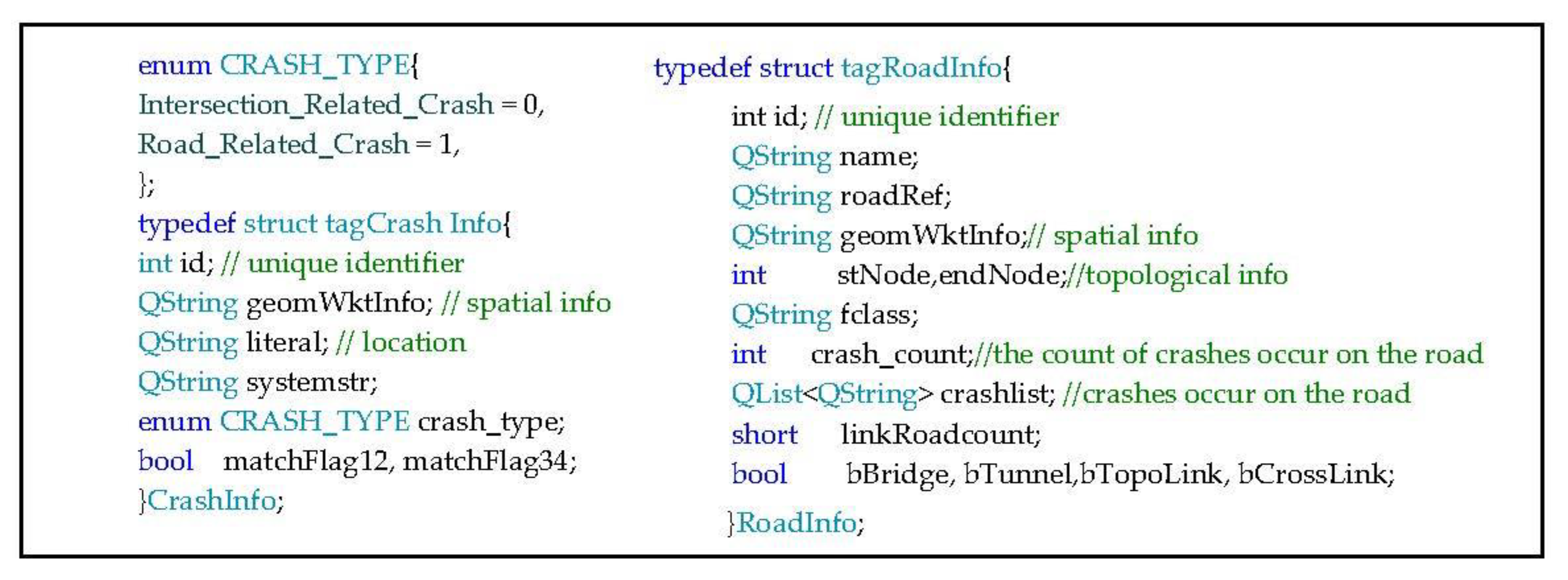
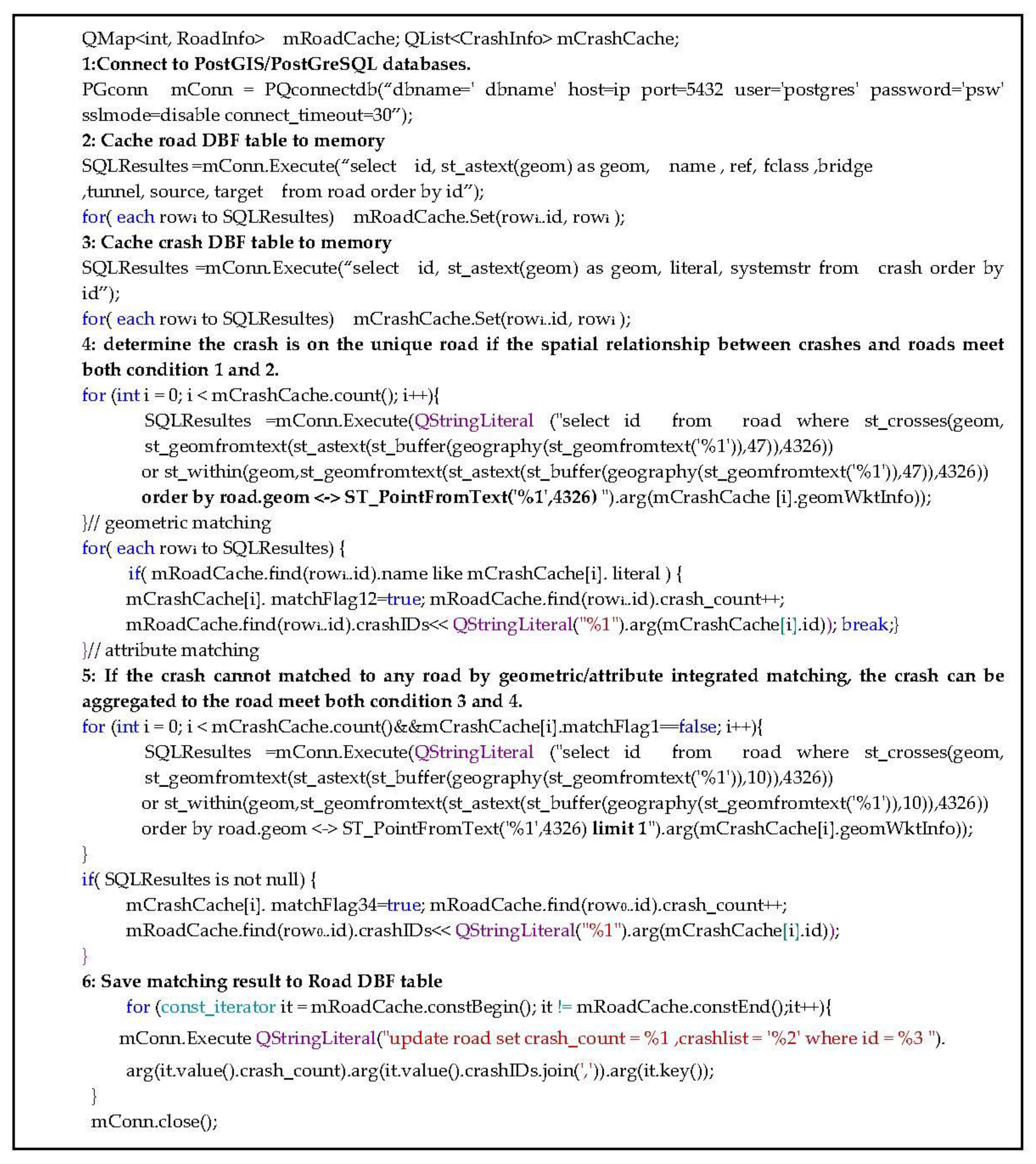
2.3.1. Crash Spatial Aggregation Algorithm

To find the RCHC, we should aggregate crashes in roads as the count of traffic crashes on the road. First, we add a fields (<crash_count>, <crashlist >) of the road DBF table. Second, we calculate the attributes (<crash_count>, <crashlist>) for each road. To determine whether the crash is on a road, the following two premises shall be considered.
Premise 1
As the accuracy of crash global positioning system (GPS) coordinate has a positioning error of approximately 10 m [34]. A crash occurs on the road if its coordinates are within 10 m of the buffer of the linear road considering the positioning error of crash.
Premise 2
As the Interstate Highway standards for the U.S. Interstate Highway System use a 12 foot (3.7 m) standard lane width [35], a crash occurring on the road can be determined if its coordinates are within 3.7 m of the buffer of the road.
Under above premises, we can determine the crash is on the road if the geometric and attribute relationships between crash and road meet both conditions 1 and 2 (means geometric and attribute integrated matching). If the crash cannot match any road by geometric and attribute integrated matching, the crash can be spatially aggregated to the road meet both conditions 3 and 4 (means spatial fuzzy matching).
  • Condition 1: The shortest distance between traffic crash and road less than 47 m (consider 10 lane roads and GPS positioning accuracy) order by the distance.
  • Condition 2: Attribute matching between name of road and location of crash.
  • Condition 3: The shortest distance between traffic crash and road is less than 10 m (consider GPS positioning accuracy).
  • Condition 4: The shortest distance between traffic crash and road is minimum in all datasets.
We use qt platform to realize the crash spatial aggregation algorithm in PostGIS/PostGreSQL database following the conditions. Figure 2 shows the definition of main data types. Figure 3 shows the main structure of the algorithm.

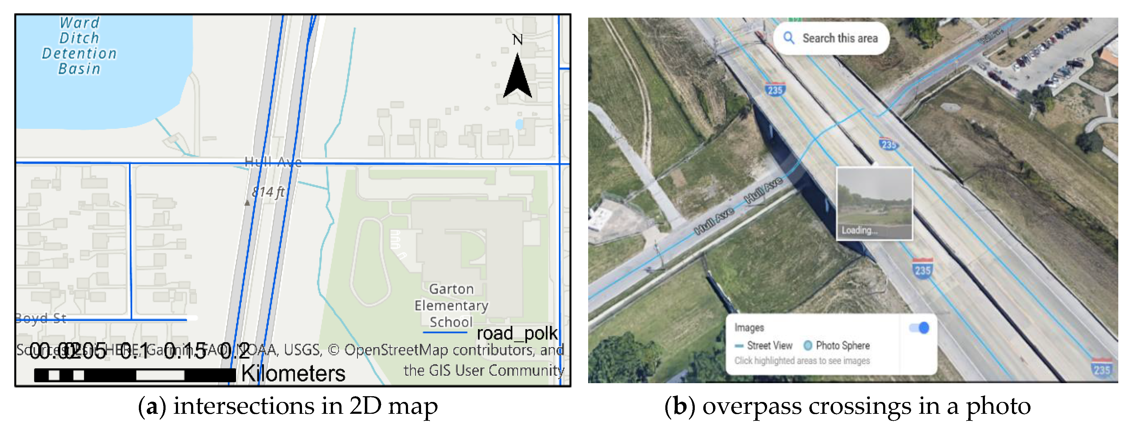
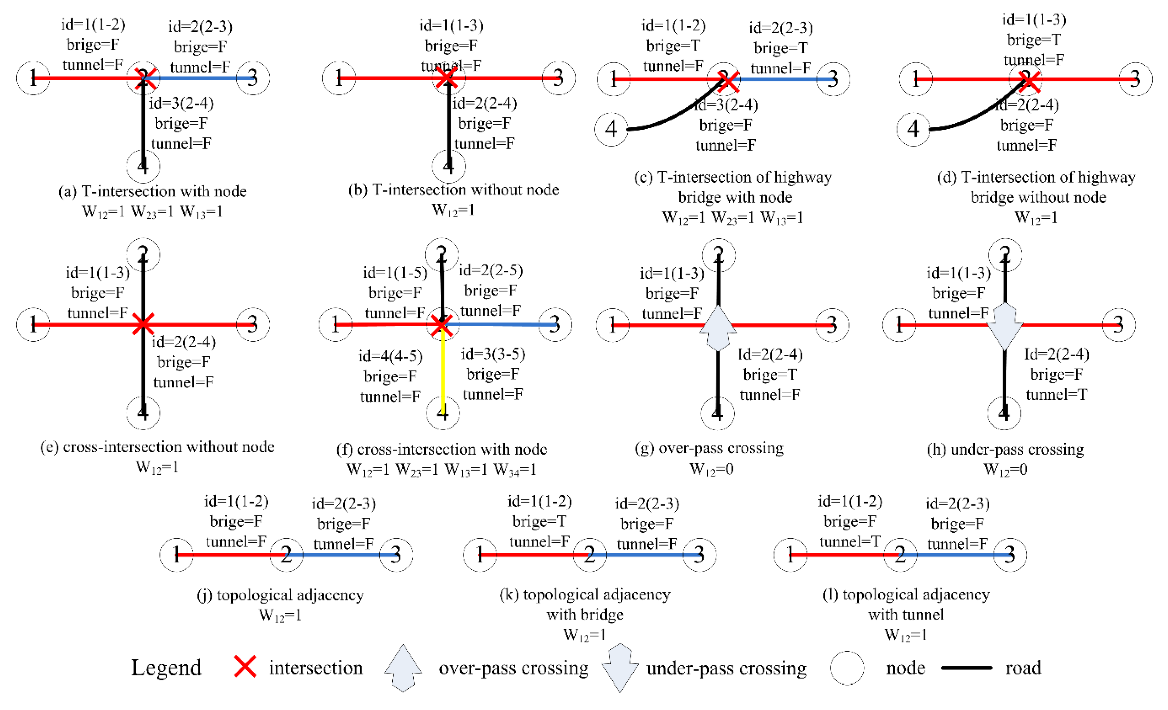
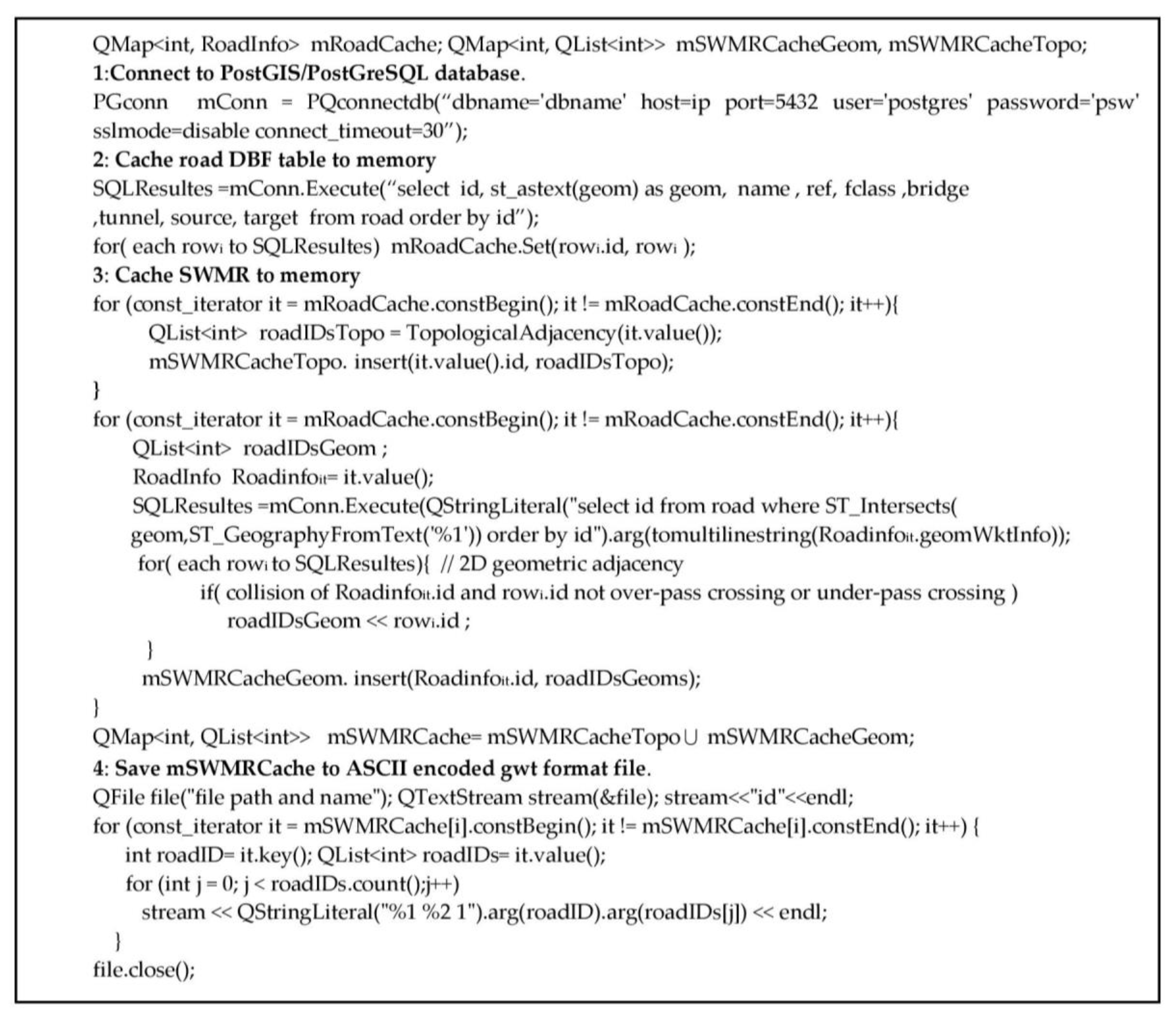
2.3.2. SWMR Construction Algorithm

A spatial weight matrix (SWM) is a representation of the spatial structure of the data, and it is designed to generate, store, reuse, and share the conceptualization of the relationships among a set of features [36]. A SWM is the key input parameters in cluster and outlier analysis. The input SWM directly determines the correctness of the calculation results of cluster and outlier analysis. Consequently, when using an inappropriate SWM, cluster and outlier analysis cannot be trusted in general.
As taking linear roads as the research object in this paper, we need to build the SWMR that matches with spatial distribution characteristics of roads for identification of RCHC by using cluster and outlier analysis. Conceptually, the SWMR is an N×N matrix (as shown in Equation (1) [26,27]. There is one row for every road and one column for every road.
SWMR = 1 2 j n 1 W 11 W 12 W 1 j W 1 n 2 W 21 W 22 W 2 j W 2 n i W i 1 W i 1 W i j W i n n W n 1 W n 2 W n j W n n
where N is the number of roads; i, j is the unique identifier of roads; and Wij is the weight of matrix (means the cell value for any given row i and column j combination) that quantifies the spatial relationship between roads.
Typically, Wij in SWMR are defined using Euclidean distance measurements and contiguity, fixed, or inverse distance weighting schemes [37,38]. However, road traffic system with crashes is based on road network which has complex topology and geometric relationships [39,40]. For identification of RCHC, defining spatial relationships in terms of road network is more appropriate.
SWMR models road spatial relationships and should follow the topology between roads that are restricted to the adjacency of road network. At the most basic level, there is a binary strategy for creating Wij to quantify the spatial relationships among roads. If the road i is a 1st-order neighbor to road j in the road network, then Wij = 1, else then Wij = 0.
In this paper, we consider topological or geometric adjacency roads, which share the same intersection or the same node, equal to 1st-order neighbors. That means there is a topological or geometric adjacency between road i and road j, then Wij = 1; otherwise, Wij = 0 using binary strategy. However, to find the geometric or topological adjacency roads is a difficult problem since the different road types (e.g., highway, local, bridge, and tunnel) in real road network have complex topological and geometric relationships. Note that roads with an overpass crossing or underpass crossing lack a true intersection. For instance, Hul Ave and I235 highway have two intersections in the 2D map; however, they do have two overpass crossings (nonintersecting) in the photo, as shown in Figure 4.
In GIS, there are different ways to model the topological and geometric relationship of road network in real world. A total of 11 kinds of graphs were summarized in this paper, as shown in Figure 5, to demonstrate the typical topological and geometric relationships of road network. Considering the typical topological and geometric relationships of road network, we can find the geometric or topological adjacency roads to calculate spatial weights of SWMR:
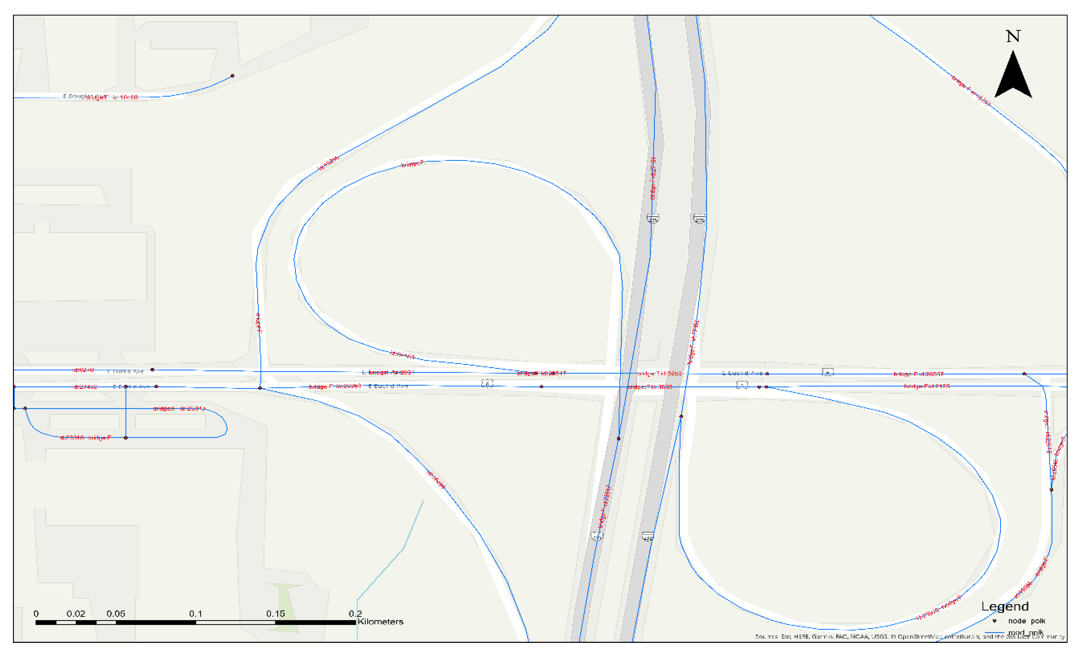
  • The spatial weights of SWMR are 1 if the roads are topological adjacent for the following cases. (a) T-intersection with node, (c) T-intersection of highway bridge with node, (f) cross-intersection with node, (j) topological adjacency, (k) topological adjacency with bridge, and (l) topological adjacency with tunnel.
  • The spatial weights of SWMR are 1 if the roads are geometric adjacent for the following cases. (b) T-intersection without node, (d) T-intersection of highway bridge without node, and (e) cross-intersection without node.
  • The spatial weights of SWMR are 0 if the roads are neither geometric adjacent nor non topological adjacent for the following cases; (g) overpass crossing and (h) underpass crossing.
Figure 6 shows the main structure of the SWMR construction algorithm.

2.3.3. Cluster and Outlier Analysis (Local Moran’s I)

The First Law of Geography [41], according to Professor Waldo Tobler, is “everything is related to everything else, but near things are more related than distant things.” Based on the first law of geography, geographical phenomena or attributes are related to each other in spatial distribution, have spatially related characteristics; that is, the closer the distance is, the more similar the things are [41]. Therefore, there are three types of distributions of crashes: dispersed, random, or clustered.
The global Moran’s I developed by Professor Moran in 1948, is one of the most preferred measure of spatial autocorrelation [42]. The global Moran’s I use a single index to detect the degree of autocorrelation of the same variable in the spatial region, and can verify the spatial distribution pattern in entire spatial extent.
In this study, the local Moran’s I (suggested in Professor Anselin based on global Moran’s I) [19] is used as a local indicator of spatial autocorrelation to find RCHC. The local Moran’s I, one of the most widely used local indicators of spatial association statistics [16], is calculated for each road to reveal the degree of spatial autocorrelation and is used to analyze whether the same variable (<crash_count> in this research) has autocorrelation at a specific local location. The local Moran’s I index is expressed as [19,22,42]
I i = X i X ¯ S i 2 j = 1 , j i n W i j ( X j X ¯ )
where Ii is the calculated local Moran’s I index of Road i. Ii is a relative measure and can only be interpreted within the context of its computed z-score or p-value. The p-value is a probability, a type of statistics to express confidence level. The z-score is a standardized local Moran’s I index. Wij is the weight in SWMR (as discussed in Section 2.3.2) that quantifies the spatial relationship between road i and road j. xi, xj is the crash count (as discussed in Section 2.3.1) of road i and road j. X ¯ is the average crash count of all roads. n is the total number of roads, i = 1, 2; n and j = 1, 2, n. Si2 is the measure of sample variance, defined as
S i 2 = j = 1 , j i n X i 2 ( X j X ¯ ) 2 n 1
In the cluster and outlier analysis, it is necessary to make assumptions about the spatial distribution of crashes, which is randomization null hypothesis of spatial distribution. The test of randomization null hypothesis of spatial distribution can be performed based on the z-score and p-value along with the local Moran’s I index. The equation to calculate the z-score ( Z I i ) for Ii is shown as
Z I i = I i E [ I i ] V [ I i ]
where E [ I i ] = j = 1 , j i n W i j n 1 , and V[Ii] = E[Ii2] − E[Ii]2.
The Zi-score is a standardized local Moran’s I value of road i. The z-scores and p-values for roads are measures of statistical significance which tell us whether or not to reject the randomization null hypothesis, road by road [1]. In this study, p-value ≤ 0.05 (95% confidence level) is used to indicate significant clusters, which is applied to each road. For either road, if its p-value is smaller than 0.05 and z-score is greater than 1.96 or less than −1.96, that road will be considered as one of the cluster or outlier. The road who z-score is positive and greater than 1.96 and p-value is smaller than 0.05, with the neighboring roads have similar z-score and p-value, form the high–high road clusters. The high–high road clusters are the RCHC, which can be used to directly identify the dangerous roads.

3. Data Description

This study focuses on the Polk County, Iowa, United States. Based on the 2010 census, its population was 430,640, representing 14% of the state’s residents, making it the Iowa’s most populous county. The study considers all types of roads (e.g., local, highway, bridge, and tunnel) and crashes occur on road (not in intersection) within the Polk County boundary. The data can be downloaded from the website: https://geodata.iowa.gov/dataset/county-boundaries-iowa.

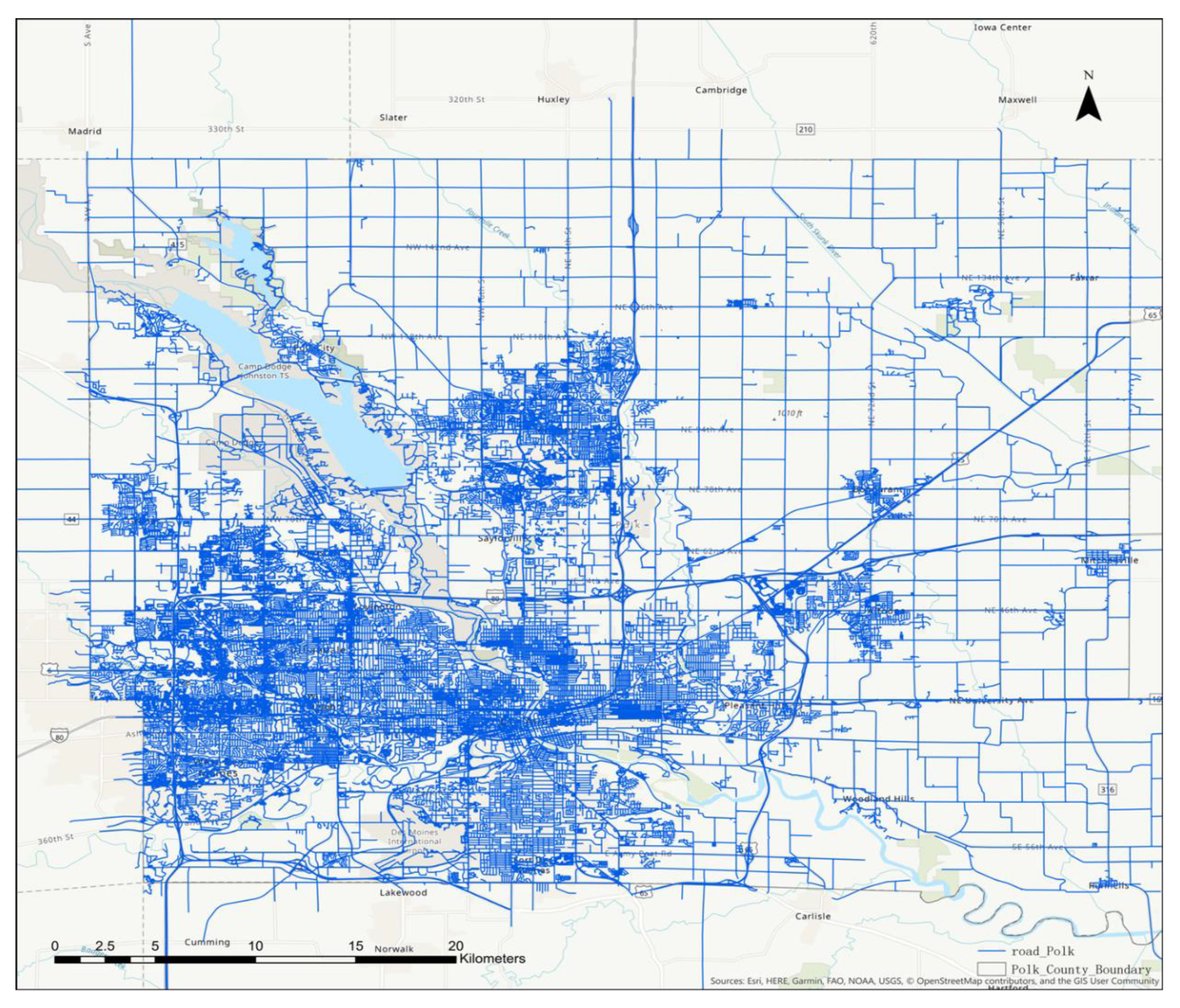
3.1. The Spatial Data of Roads

The spatial data of IOWA statewide roads that this study employ can be download form OpenStreetMap [43] website (http://download.geofabrik.de/north-america.html). We extract spatial data of roads from the Iowa statewide road using (a) select layer by location tool (roads intersect with the Polk County boundary) and (b) select layer by attribute (roads suitable for cars) from ArcGIS geoprocessing tool box. A total of 27,606 roads are successfully recorded in ArcGIS software, as shown in Figure 7.
Note that the road shapefile of other cities or regions can be easily downloaded from Geofabrik’s free download server, which has the latest global spatial road data normally update every day from the OpenStreetMap project.

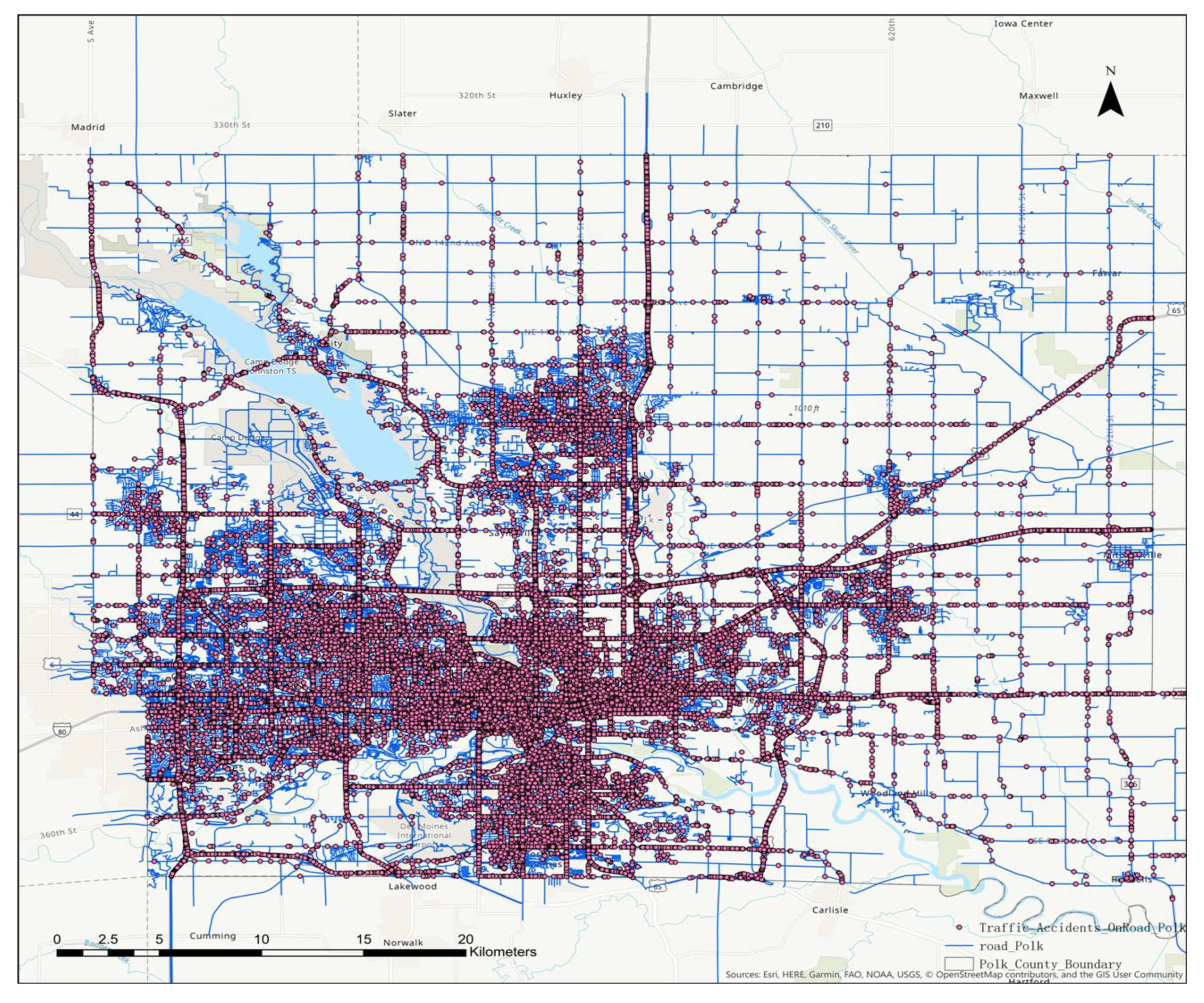
3.2. The Spatial Data of Road-Related Crashes

This study employs the spatial data of crashes provided by the Iowa Department of Transportation’s public platform (https://data.iowadot.gov/), which has the statewide data of general traffic crashes from the prior 10 years.
The database of crashes contains 49 types of information (e.g., crash_key, casenumber, crash_day, crash_date, district, county_num, literal, locfsthrm, locfsthrm, light, weather, rdtype, xcoord, and ycoord). For this study, a dataset of road-related crashes that occurred in Polk County was selected and analyzed.
We extract spatial data of crashes of the Polk County from the Iowa statewide traffic crash shapefile using (a) select layer by location tool (crashes intersect with the Polk County boundary) and (b) select layer by attribute tool (crashes are not intersection-related) from ArcGIS geo-processing tool box. A total of 41,734 road-related crashes that happened in Polk County from 1 January 2008–6 August 2018 are successfully recorded in ArcGIS, as shown in Figure 8.
Note that we can also access other cities or regions crash shapefile published by state Department of Transportation in USA using the same extracting method.

4. Results and Discussion

4.1. The SWMR of Polk County

As described earlier, SWMR is the critical input parameters for the local Moran’s I analysis. Therefore, it is necessary to establish the SWMR of the Polk County to accurately express the spatial relationship between roads.
As discussed in Section 2.2.3, we use ASCII encoded gwt format file to store SWMR data. The first line of the file of the SWMR in gwt format is the name of the unique identifier field (we use the field ‘ID’ as the unique identifier field in this paper). The spatial weight (Wij) is calculated by considering topological and geometric relationships between roads. Due to space limitations, we take the typical highway–local link road graph shown in Figure 9 as an example to demonstrate the SWMR of Polk County.
Table 2 lists the content of the ASCII encoded gwt format file of roads, including motorway links (ID. 23970, 24103) and bridges (ID. 3833, 3950) created by the algorithm of constructing of SWMR (discussed in Section 2.3.2), to save the conceptualization data of road spatial relationships. It should be noted that the SWMR is a sparse matrix, and there is a large amount of zero Wij data. Therefore, in this paper, the rows with a spatial weight of 0 are omitted since the default setting for spatial weights is 0 in the spatial data mining approach, which can effectively reduce the file storage space.

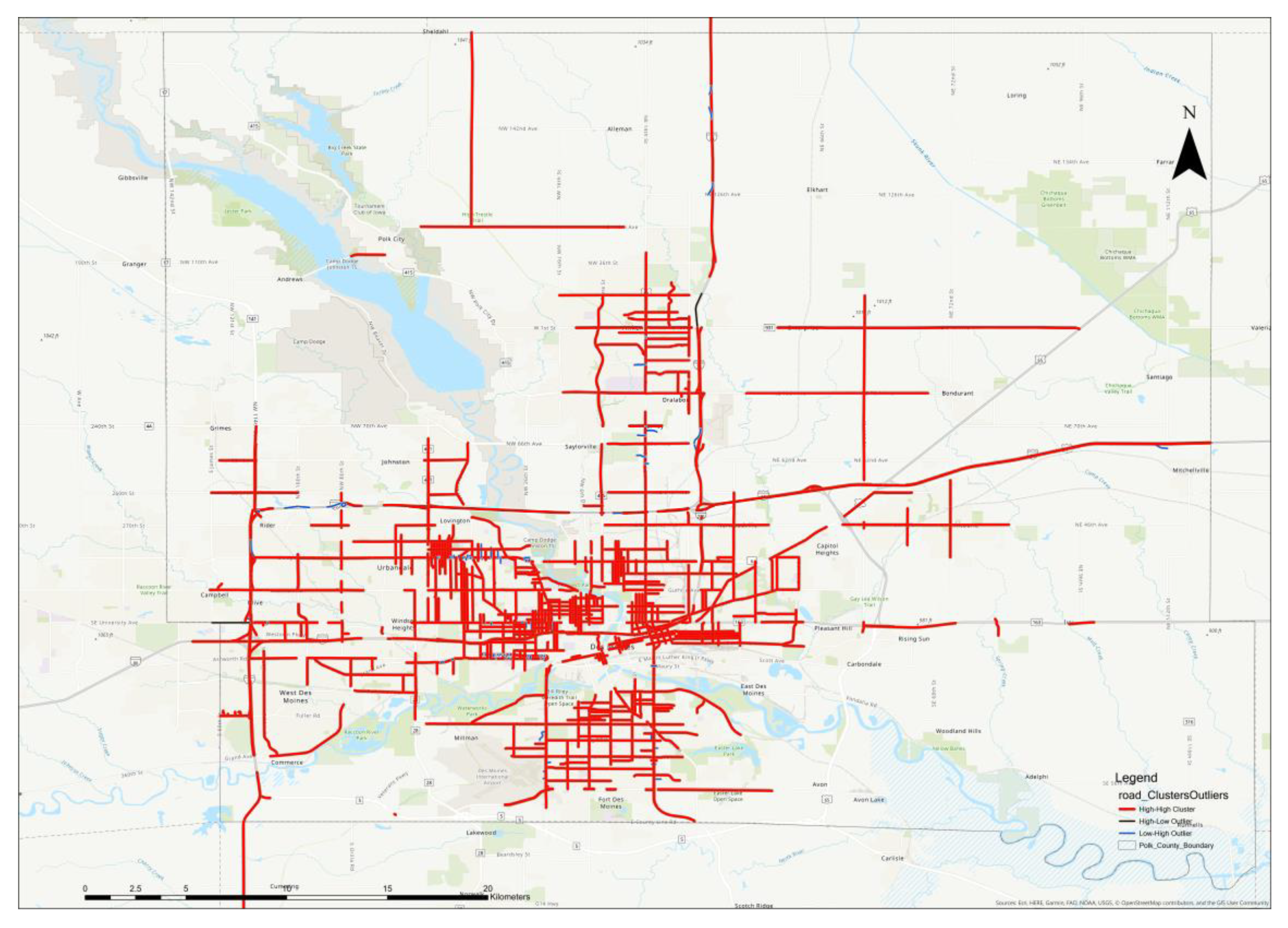
4.2. The Results of Road Cluster and Outlier Analysis of Polk County

The study uses cluster and outlier analysis (the local Moran’s I, as discussed in Section 2.3.3) from geo-processing tools in ArcGIS [44,45], by taking the following input parameters, as shown in Table 3, to calculate local Moran’s I index, z-score, and p-value for each linear road to obtain road clusters and outliers across Polk County.
All roads should have at least one neighbor [32] according to the best practice guidelines of cluster and outlier analysis. In this research, a total of 27,491 roads were selected in the input feature class since we find 115 roads in OpenStreetMap roads of Polk County have no neighbor when we construct the SWMR of Polk County.
In general, there are four types of road cluster and outlier in the road cluster and outlier shapefile, as discussed in Section 2.2.3: high–high cluster (cotype is HH), low-low cluster (cotype is LL), high–low outlier (cotype is HL), and low–high outlier (cotype is HL). The high–high cluster, high–low outlier, and low–high outlier are colored in red, black, and blue, respectively. The results, as shown in Figure 10 using map visualization, clearly demonstrate the road clusters and outliers.
High–high road cluster indicates that there is a positive autocorrelation. The roads in this cluster all have high crashes and the neighbor roads also have high-frequency crashes. That means, High–high road cluster is the RCHC that we should identify from the 27,606 roads of Polk County.
The RCHC of Polk County, as shown in Figure 10, centered along with I 35, I235, US69, I80, and US 6, can be discovered is relevant to hazardous roads detection. There are 738 roads in the RCHC of Polk County, which account for 2.67% of all roads and 24, 652 crashes occurred in RCHC, accounting for 59.07% of all crashes. That means 59.07% crashes occurred in 2.67% roads in Polk County. In addition, we can discovery that 85.60% crashes in RCHC occurred on major roads, including motorway, trunk, primary, secondary, and tertiary, as shown in Figure 11. We can quantitatively identify that 59.07% crashes of Polk County have strong positive spatial autocorrelation with topological or geometric adjacency of roads.
Portion of calculated local Moran’s I, z-score, and p-value for each road in RCHC are shown in Table 4, based on which, transportation authorities can develop targeted mitigation strategies for the roads in RCHC to effectively reduce the number of crashes.
The high–low and low–high outlier shows that there is a negative autocorrelation. The roads in high–low outlier have high-frequency crashes; however, their neighboring roads have low-frequency crashes. Contrarily, the roads in low–high outlier have low-frequency crashes; however, their neighboring roads have high-frequency crashes. A portion of the calculated local Moran’s I, z-score, and p-value of each road in low–high and high–low outlier are shown in Table 5. Transportation authorities should also pay attention to roads in high–low and low–high outliers to find why there is a negative autocorrelation.

5. Recommendation of Future Work

In this paper, we have developed a spatial data mining approach to directly identify road clusters with high-frequency crashes (RCHC) by using spatial weight matrix of roads (SWMR) and the local Moran’s I for cluster and outlier analysis. We believe that the proposed approach can be extended to the following fields, which can be considered as future work.

5.1. Spatiotemporal Data Mining Approach.

In this study, the ten-year crashes were equally applied in spatial data mining approach. However, different temporal crash factors, such as light, season, weather, may be varied. It is necessary to differentiate the treatment of crashes according to different temporal factors. As such, we will develop the spatiotemporal data mining approach considering the several spatiotemporal correlations between the crashes and main factors to discover the spatial and temporal patterns of traffic crashes according to different factors.

5.2. Identify Traffic Bottleneck.

In recent years, identify traffic patterns, including traffic bottlenecks, has received much attention [46,47,48]. The proposed approach in this paper has the potential to identify the traffic bottleneck. The spatial relationship between the bottleneck and broad network can be established by a fuzzy spatial aggregation algorithm, and the spatial weight matrix of road network are then used to study the degree of autocorrelation of the traffic congestion and discover the spatial distribution pattern of the traffic bottleneck under the constraints of the road network.

5.3. Identify Certain Roadway Damages.

Due to various adverse factors, such as pounding and impact [49], chloride diffusion [50] and corrosion [51,52], and freeze and thaw [53,54], roadways are subject damages, such as potholes and cracks, which will negatively impact traffic flow [55], generating abnormal traffic patterns, such as sudden slow down and lane changes, which will worsen over time. Therefore, a spatiotemporal data mining approach by using the historical data will be developed. Cluster and outlier analysis can be used to discover roadway damages by checking the degree of autocorrelation of traffic flow and the outliers represent with abnormal traffic flow.

5.4. Cloud-Based RCHC Identification

The proposed approach was developed and validated using a personal computer that has the capacity to identify RCHC in large cities or regions with populations of ~430,000 people, such as Polk County; however, it is difficult to process the big data of crashes and roads in megacities. As a future work, we will deploy, test, and amend the proposed approach in the cloud computing environment [56] to provide high performance computing solutions for identify RCHC in megacities, to further improve the data processing capability of this approach.

6. Conclusions

As important carriers of traffic, roads and their ancillary facilities have important impacts on the frequency of crashes [57,58]. This paper successfully demonstrates a spatial data mining approach to directly identify road clusters with high-frequency crashes (RCHC). The application of methodology was illustrated by using the spatial data set (stored in SHP file format) including traffic crashes (2008–2018) and roads of Polk County, Iowa, U.S.A. The proposed crash spatial aggregation algorithm uses geometric and attribute integrated matching and spatial fuzzy matching to build the crash–road spatial relationships considering GPS location accuracy. The developed spatial weight matrix of roads (SWMR) algorithm has the ability to detect and accommodate overpass crossing and underpass crossing with the consideration of the 11 typical topological and geometric relationships of roads. The algorithm, creates accurate SWMR of complex road network, have the added value that can support further spatial statistics (e.g., high–low clustering and Getis-Ord Gi* analysis) of road network crashes. As a major contribution, the research adopts a new idea and focuses on line-based local Moran’s I analysis by taking line-based roads as the core research objects instead of point-based crashes. As a result, the proposed method can directly identify RCHC.

Author Contributions

Z.Z. and G.S. developed the original idea. Z.Z. and Y.M. proposed the method. Z.Z. and Y.M. analyzed the data. Z.Z., G.S., and Y.M. wrote the paper.

Funding

This work was supported by the Construction Science and Technology Program of Hubei Province in 2016 (Transportation, municipal No. 02) and the Research Start-Up Funding of Hubei University of Education Grant NO. 18RC09.

Conflicts of Interest

The authors declare no conflicts of interest.

References

  1. Harirforoush, H.; Bellalite, L.; Bénié, G.B. Spatial and Temporal Analysis of Seasonal Traffic Accidents. Am. J. Traffic Transp. Eng. 2019, 4, 7–16. [Google Scholar] [CrossRef] [Green Version]
  2. Pelaez, C.G.A.; Garcia, F.; de la Escalera, A.; Armingol, J.M. Driver Monitoring Based on Low-Cost 3-D Sensors. IEEE Trans. Intell. Transp. Syst. 2014, 15, 1855–1860. [Google Scholar] [CrossRef] [Green Version]
  3. Carmona, J.; García, F.; Martín, D.; Escalera, A.; Armingol, J. Data Fusion for Driver Behaviour Analysis. Sensors 2015, 15, 25968–25991. [Google Scholar] [CrossRef] [PubMed] [Green Version]
  4. Han, J.; Kamber, M.; Pei, J. Data Mining: Concepts and Techniques; Elsevier/Morgan Kaufmann: Amsterdam, The Netherland; Boston, MA, USA, 2012; ISBN 978-0-12-381480-7. [Google Scholar]
  5. Kumar, S.; Toshniwal, D. A data mining framework to analyze road accident data. J. Big Data 2015, 2, 26. [Google Scholar] [CrossRef] [Green Version]
  6. Chen, F.; Deng, P.; Wan, J.; Zhang, D.; Vasilakos, A.V.; Rong, X. Data Mining for the Internet of Things: Literature Review and Challenges. Int. J. Distrib. Sens. Netw. 2015, 11, 431047. [Google Scholar] [CrossRef] [Green Version]
  7. Kumar, S.; Toshniwal, D.; Parida, M. A comparative analysis of heterogeneity in road accident data using data mining techniques. Evol. Syst. 2017, 8, 147–155. [Google Scholar] [CrossRef]
  8. Castro, Y.; Kim, Y.J. Data mining on road safety: Factor assessment on vehicle accidents using classification models. Int. J. Crashworthiness 2016, 21, 104–111. [Google Scholar] [CrossRef]
  9. Taamneh, M.; Alkheder, S.; Taamneh, S. Data-mining techniques for traffic accident modeling and prediction in the United Arab Emirates. J. Transp. Saf. Secur. 2017, 9, 146–166. [Google Scholar] [CrossRef]
  10. Li, L.; Shrestha, S.; Hu, G. Analysis of road traffic fatal accidents using data mining techniques. In Proceedings of the 2017 IEEE 15th International Conference on Software Engineering Research, Management and Applications (SERA), London, UK, 7–9 June 2017; IEEE: London, UK, 2017; pp. 363–370. [Google Scholar] [CrossRef]
  11. Soltani, A.; Askari, S. Exploring spatial autocorrelation of traffic crashes based on severity. Injury 2017, 48, 637–647. [Google Scholar] [CrossRef]
  12. Shekhar, S.; Jiang, Z.; Ali, R.; Eftelioglu, E.; Tang, X.; Gunturi, V.; Zhou, X. Spatiotemporal Data Mining: A Computational Perspective. ISPRS Int. J. Geo-Inf. 2015, 4, 2306–2338. [Google Scholar] [CrossRef]
  13. Zheng, Y. Trajectory Data Mining: An Overview. ACM Trans. Intell. Syst. Technol. 2015, 6, 29. [Google Scholar] [CrossRef]
  14. Chen, W.; Panahi, M.; Pourghasemi, H.R. Performance evaluation of GIS-based new ensemble data mining techniques of adaptive neuro-fuzzy inference system (ANFIS) with genetic algorithm (GA), differential evolution (DE), and particle swarm optimization (PSO) for landslide spatial modelling. Catena 2017, 157, 310–324. [Google Scholar] [CrossRef]
  15. Ouni, F.; Belloumi, M. Pattern of road traffic crash hot zones versus probable hot zones in Tunisia: A geospatial analysis. Accid. Anal. Prev. 2019, 128, 185–196. [Google Scholar] [CrossRef]
  16. Xie, Z.; Yan, J. Detecting traffic accident clusters with network kernel density estimation and local spatial statistics: An integrated approach. J. Transp. Geogr. 2013, 31, 64–71. [Google Scholar] [CrossRef]
  17. Blazquez, C.A.; Celis, M.S. A spatial and temporal analysis of child pedestrian crashes in Santiago, Chile. Accid. Anal. Prev. 2013, 50, 304–311. [Google Scholar] [CrossRef]
  18. Zhang, T.; Lin, G. On Moran’s I coefficient under heterogeneity. Comput. Stat. Data Anal. 2016, 95, 83–94. [Google Scholar] [CrossRef]
  19. Anselin, L. Local Indicators of Spatial Association-LISA. Geogr. Anal. 2010, 27, 93–115. [Google Scholar] [CrossRef]
  20. Jana, M.; Sar, N. Modeling of hotspot detection using cluster outlier analysis and Getis-Ord Gi * statistic of educational development in upper-primary level, India. Model. Earth Syst. Environ. 2016, 2, 60. [Google Scholar] [CrossRef] [Green Version]
  21. Mitra, S. Spatial Autocorrelation and Bayesian Spatial Statistical Method for Analyzing Intersections Prone to Injury Crashes. Transp. Res. Rec. 2009, 2136, 92–100. [Google Scholar] [CrossRef]
  22. Yuan, Y.; Cave, M.; Zhang, C. Using Local Moran’s I to identify contamination hotspots of rare earth elements in urban soils of London. Appl. Geochem. 2018, 88, 167–178. [Google Scholar] [CrossRef]
  23. Soltanolkotabi, M.; Candés, E.J. A geometric analysis of subspace clustering with outliers. Ann. Stat. 2012, 40, 2195–2238. [Google Scholar] [CrossRef]
  24. Hashimoto, S.; Yoshiki, S.; Saeki, R.; Mimura, Y.; Ando, R.; Nanba, S. Development and application of traffic accident density estimation models using kernel density estimation. J. Traffic Transp. Eng. 2016, 3, 262–270. [Google Scholar] [CrossRef] [Green Version]
  25. Anderson, T.K. Kernel density estimation and K-means clustering to profile road accident hotspots. Accid. Anal. Prev. 2009, 41, 359–364. [Google Scholar] [CrossRef] [PubMed]
  26. Mawarni, M.; Machdi, I. Dynamic nearest neighbours for generating spatial weight matrix. In Proceedings of the 2016 International Conference on Advanced Computer Science and Information Systems (ICACSIS), Malang, Indonesia, 15–16 October 2016; IEEE: Malang, Indonesia, 2016; pp. 257–262. [Google Scholar] [CrossRef]
  27. Qu, X.; Lee, L. Estimating a spatial autoregressive model with an endogenous spatial weight matrix. J. Econom. 2015, 184, 209–232. [Google Scholar] [CrossRef]
  28. Ermagun, A.; Levinson, D. An introduction to the network weight matrix. Geogr. Anal. 2018, 50, 76–96. [Google Scholar] [CrossRef]
  29. Obe, R.O.; Hsu, L.S. PostgreSQL: Up and Running, 2nd ed.; O’Reilly: Sebastopol, CA, USA, 2014; ISBN 978-1-4493-7319-1. [Google Scholar]
  30. Bogorny, V.; Avancini, H.; de Paula, B.C.; Kuplich, C.R.; Alvares, L.O. Weka-STPM: A Software Architecture and Prototype for Semantic Trajectory Data Mining and Visualization. Trans. GIS 2011, 15, 227–248. [Google Scholar] [CrossRef]
  31. Singh, P.S.; Lyngdoh, R.B.; Chutia, D.; Saikhom, V.; Kashyap, B.; Sudhakar, S. Dynamic shortest route finder using pgRouting for emergency management. Appl. Geomat. 2015, 7, 255–262. [Google Scholar] [CrossRef]
  32. Scott, L.M.; Janikas, M.V. Spatial Statistics in ArcGIS. In Handbook of Applied Spatial Analysis; Fischer, M.M., Getis, A., Eds.; Springer: Berlin/Heidelberg, Germany, 2010; pp. 27–41. ISBN 978-3-642-03646-0. [Google Scholar] [CrossRef]
  33. Anselin, L.; Syabri, I.; Kho, Y. GeoDa: An Introduction to Spatial Data Analysis. Geogr. Anal. 2006, 38, 5–22. [Google Scholar] [CrossRef]
  34. Wing, M.G.; Eklund, A.; Kellogg, L.D. Consumer-Grade Global Positioning System (GPS) Accuracy and Reliability. J. For. 2005, 103, 169–173. [Google Scholar] [CrossRef]
  35. Khan, M.; Abdel-Rahim, A.; Williams, C.J. Potential crash reduction benefits of shoulder rumble strips in two-lane rural highways. Accid. Anal. Prev. 2015, 75, 35–42. [Google Scholar] [CrossRef]
  36. Getis, A.; Aldstadt, J. Constructing the Spatial Weights Matrix Using a Local Statistic. Geogr. Anal. 2004, 36, 90–104. [Google Scholar] [CrossRef]
  37. Seya, H.; Yamagata, Y.; Tsutsumi, M. Automatic selection of a spatial weight matrix in spatial econometrics: Application to a spatial hedonic approach. Reg. Sci. Urban Econ. 2013, 43, 429–444. [Google Scholar] [CrossRef]
  38. Getis, A. Spatial interaction and spatial autocorrelation: A cross-product approach. Environ. Plan. A Econ. Space 1991, 23, 1269–1277. [Google Scholar] [CrossRef]
  39. Liu, H.; Wang, J. Vulnerability assessment for cascading failure in the highway traffic system. Sustainability 2018, 10, 2333. [Google Scholar] [CrossRef] [Green Version]
  40. Du, B.; Huang, R.; Chen, X.; Xie, Z.; Liang, Y.; Lv, W.; Ma, J. Active CTDaaS: A data service framework based on transparent IoD in city traffic. IEEE Trans. Comput. 2016, 65, 3524–3536. [Google Scholar] [CrossRef]
  41. Tobler, W. On the First Law of Geography: A Reply. Ann. Assoc. Am. Geogr. 2004, 94, 304–310. [Google Scholar] [CrossRef]
  42. Kumari, M.; Sarma, K.; Sharma, R. Using Moran’s I and GIS to study the spatial pattern of land surface temperature in relation to land use/cover around a thermal power plant in Singrauli district, Madhya Pradesh, India. Remote Sens. Appl. Soc. Environ. 2019, 15, 100239. [Google Scholar] [CrossRef]
  43. Haklay, M.; Weber, P. OpenStreetMap: User-Generated Street Maps. IEEE Pervasive Comput. 2008, 7, 12–18. [Google Scholar] [CrossRef] [Green Version]
  44. Aghajani, M.A.; Dezfoulian, R.S.; Arjroody, A.R.; Rezaei, M. Applying GIS to Identify the Spatial and Temporal Patterns of Road Accidents Using Spatial Statistics (case study: Ilam Province, Iran). Transp. Res. Procedia 2017, 25, 2126–2138. [Google Scholar] [CrossRef]
  45. Estiri, H. Tracking Urban Sprawl: Applying Moran’s I Technique in Developing Sprawl Detection Models. In Proceedings of the 43rd Annual Conference of the Environmental Design Research Association EDRA, Seattle, WA, USA, 30 May–2 June 2012; pp. 47–53. [Google Scholar]
  46. Zheng, Z.; Ahn, S.; Chen, D.; Laval, J. Applications of wavelet transform for analysis of freeway traffic: Bottlenecks, transient traffic, and traffic oscillations. Transp. Res. Part B Methodol. 2011, 45, 372–384. [Google Scholar] [CrossRef] [Green Version]
  47. Du, B.; Zhou, W.; Liu, C.; Cui, Y.; Xiong, H. Transit pattern detection using tensor factorization. Inf. J. Comput. 2019, 31, 193–206. [Google Scholar] [CrossRef]
  48. Ma, X.; Luan, S.; Du, B.; Yu, B. Spatial copula model for imputing traffic flow data from remote microwave sensors. Sensors 2017, 17, 2160. [Google Scholar] [CrossRef] [PubMed] [Green Version]
  49. Xu, B.; Song, G.; Mo, Y. Embedded piezoelectric lead-zirconate-titanate-based dynamic internal normal stress sensor for concrete under impact. J. Intell. Mater. Syst. Struct. 2017, 28, 2659–2674. [Google Scholar] [CrossRef]
  50. Peng, J.; Hu, S.; Zhang, J.; Cai, C.S.; Li, L. Influence of cracks on chloride diffusivity in concrete: A five-phase mesoscale model approach. Constr. Build. Mater. 2019, 197, 587–596. [Google Scholar] [CrossRef]
  51. Li, W.; Xu, C.; Ho, S.; Wang, B.; Song, G. Monitoring concrete deterioration due to reinforcement corrosion by integrating acoustic emission and fbg strain measurements. Sensors 2017, 17, 657. [Google Scholar] [CrossRef] [Green Version]
  52. Peng, J.; Xiao, L.; Zhang, J.; Cai, C.S.; Wang, L. Flexural behavior of corroded HPS beams. Eng. Struct. 2019, 195, 274–287. [Google Scholar] [CrossRef]
  53. Kong, Q.; Wang, R.; Song, G.; Yang, Z.J.; Still, B. Monitoring the soil freeze-thaw process using piezoceramic-based smart aggregate. J. Cold Reg. Eng. 2014, 28, 06014001. [Google Scholar] [CrossRef]
  54. Wang, Y.; Tan, Y.; Guo, M.; Wang, X. Influence of Emulsified Asphalt on the Mechanical Property and Microstructure of Cement-Stabilized Gravel under Freezing and Thawing Cycle Conditions. Materials 2017, 10, 504. [Google Scholar] [CrossRef] [Green Version]
  55. Mao, X.; Wang, J.; Yuan, C.; Yu, W.; Gan, J. A Dynamic Traffic Assignment Model for the Sustainability of Pavement Performance. Sustainability 2018, 11, 170. [Google Scholar] [CrossRef] [Green Version]
  56. Du, B.; Huang, R.; Xie, Z.; Ma, J.; Lv, W. KID model-driven things-edge-cloud computing paradigm for traffic data as a service. IEEE Netw. 2018, 32, 34–41. [Google Scholar] [CrossRef]
  57. García, F.; García, J.; Ponz, A.; de la Escalera, A.; Armingol, J.M. Context aided pedestrian detection for danger estimation based on laser scanner and computer vision. Expert Syst. Appl. 2014, 41, 6646–6661. [Google Scholar] [CrossRef] [Green Version]
  58. García, F.; Jiménez, F.; Anaya, J.; Armingol, J.; Naranjo, J.; de la Escalera, A. Distributed pedestrian detection alerts based on data fusion with accurate localization. Sensors 2013, 13, 11687–11708. [Google Scholar] [CrossRef] [PubMed] [Green Version]
Figure 1. Process map for the approach of directly identifying road clusters with high-frequency crashes (RCHC).
Applsci 09 05282 g001
Figure 2. Definition of main data types.
Applsci 09 05282 g002
Figure 3. Structure of crash spatial aggregation algorithm.
Applsci 09 05282 g003
Figure 4. Overpass crossing (nonintersecting) of the highway and local road.
Applsci 09 05282 g004
Figure 5. Typical topological and geometric relationships of road network.
Applsci 09 05282 g005
Figure 6. Structure of the spatial weight matrix of roads (SWMR) construction algorithm.
Applsci 09 05282 g006
Figure 7. Distribution of roads in Polk County.
Applsci 09 05282 g007
Figure 8. Distribution of crashes in Polk County.
Applsci 09 05282 g008
Figure 9. Typical highway–local link road graph.
Applsci 09 05282 g009
Figure 10. Distribution of road clusters and outliers of Polk County.
Applsci 09 05282 g010
Figure 11. Statistics of crash counts in different road classes in RCHC.
Applsci 09 05282 g011
Table 1. The overview of file types.
NameFile TypeFormat TypeFeature TypeDescription
RoadInputShapefileLineThe feature file of road centerlines
CrashInputShapefilePointThe feature file of crashes
BoundaryInputShapefileRegionThe Boundary of study Area
Traffic DatabaseIntermediatePostGreSQL
Database
Line/Point/RegionThe spatial database converted
from input shapefiles
SWMR fileOutputGWT File/ASCII encoded SWM File of road
Road clusters
and outliers
OutputShapefileLineThe result of cluster and outlier analysis
Table 2. The content of the ASCII encoded gwt format file.
First Row: ID (Unique Identifier Field)
Row No.IDSiIDSjWijRow No.IDSiIDSjWij
12397021251223970173521
32410339511424103235121
524103238171624103271911
738332125183833269561
93950238171103950269571
Table 3. Input Parameters of cluster and outlier analysis (Anselin local Moran’s I).
Input ParameterInput Value
Input Feature Classroad_polk
Input Fieldcrash_count
Output Feature Classc:\data\myproject.gdb\road_clustersoutliers
Conceptualization of Spatial Relationshipsget_spatial_weights_from_file
Standardizationnone
Distance Band or Threshold Distancenone
Weights Matrix Filec:\data\swmr.gwt
Apply False Discovery Rate Correctionno_fdr
Table 4. Local Moran’s I, z-score, and p-value of roads in high–high cluster (RCHC).
IdFclassNameRefCrash_CountLocal Moran Iz-Scorep-ValueCotype
24305motorway I 35492209.1394.510.00HH
17387motorway I 235343141.9954.230.00HH
24483secondaryFleur Drive 295422.7970.280.00HH
26939motorway I 2352908.573.060.00HH
26629motorway I 80; I 3526710.704.410.00HH
27435motorway I 80; US 6262141.8558.530.00HH
26612primarySouth Ankeny BoulevardUS 69252242.9959.570.00HH
26533motorway I 80; I 35250141.8282.740.00HH
26381primaryDouglas AvenueUS 6246751.0690.180.00HH
24779secondaryUniversity Avenue 2411570.78229.300.00HH
26953motorway I 35230130.2749.760.00HH
26621motorway I 235209107.7462.860.00HH
26230primarySoutheast 14th StreetUS 69200455.7788.670.00HH
26884motorway I 8019991.3446.150.00HH
27436tertiaryIngersoll Avenue 19939.294.360.00HH
26954motorway I 3519839.2314.990.00HH
24841motorway I 35; I 801937.773.930.00HH
24971motorway I 80; I 35188160.1272.360.00HH
24800primarySoutheast 14th StreetUS 69181438.9587.030.00HH
24845motorway I 8018014.6410.460.00HH
26781secondaryUniversity Avenue 179133.6127.010.00HH
24918primarySoutheast 14th StreetUS 69177132.5650.640.00HH
26558motorway I 80; I 351727.824.560.00HH
24782primaryNortheast 14th StreetUS 6916778.7418.260.00HH
25995secondaryMartin Luther King Jr. Parkway 161378.83102.330.00HH
24849motorway I 80; I 3515572.6251.890.00HH
Table 5. Local Moran’s I, z-score, and p-value of roads in high–low and high–low outliers.
IdFclassNameCrash_CountLocal Moran iz-Scorep-ValueCotype
1970residentialWillowmere Drive0−4.91−2.480.01LH
23513tertiaryWatrous Avenue0−5.11−2.580.01LH
24306residentialWakonda Drive0−4.89−2.020.04LH
2749secondaryUniversity Avenue0−4.60−3.280.00LH
15523residentialSouthwest 16th Street0−3.86−2.250.02LH
1670residentialSouthlawn Drive0−4.95−2.890.00LH
911tertiaryPorter Avenue0−4.99−2.520.01LH
13993residentialNortheast 69th Place0−2.58−2.610.01LH
14706tertiaryMaury Street0−4.46−2.020.04LH
23514secondaryIndianola Avenue0−8.43−3.480.00LH
12238residentialHart Avenue0−5.87−3.420.00LH
10097residentialHackley Avenue0−4.86−2.010.04LH
23676tertiaryEast Watrous Avenue0−6.39−3.230.00LH
4286tertiaryCowles Drive0−4.49−2.030.04LH
4770secondaryBell Avenue0−4.63−2.090.04LH
8815tertiaryAurora Avenue0−5.08−2.100.04LH
14734residential41st Street0−3.98−2.320.02LH
1970residentialWillowmere Drive0−4.91−2.480.01LH
23513tertiaryWatrous Avenue0−5.11−2.580.01LH
24789motorwayI 35100−3.59−2.090.04HL
27604secondaryUniversity Avenue119−19.65−4.680.00HL

