Distributed and Localized Hub-Based Hierarchical Information Transmission Control in Large-Scale Wireless Cloud Networks

Abstract

This paper proposes a virtual infrastructure-based hierarchical information transmission scheme consisting of two phases, macroscopic transmission and local transmission controls. The macroscopic transmission control builds a hub-node-based virtual infrastructure and then finds the optimal hub route that satisfies the stochastic end-to-end delay constraint. Each node determines whether it belongs to a hub node by itself in a distributed manner. The local transmission control builds a robust local path between hub nodes by using the synchronized redundancy concept; this minimizes the effects of transmission failure by reducing the control traffic overhead and time to reconfigure transmission paths without rediscovery of the transmission path from the source node. Simulations confirmed that, as the network size increased, the performance of the proposed transmission scheme increased in terms of packet delivery ratio and control packet overhead. The scheme can be applied to mobile ad hoc cloud computing systems based on self-organizing vehicular networks or drone networks as a key control.

1. Introduction

The diversification and integration of computing environments of wireless mobile terminals leads to large-scale wireless networks. With this evolution, one of the major challenges is to overcome frequent topology change and design a combinatorially stable multi-hop network. Frequent topology changes make it difficult to control large-scale wireless networks and cause significant performance degradation. Moreover, in combinatorially unstable wireless networks, global topology update messages lead to incorrect network topology by delivering imprecise information, thereby preventing loop-free path discovery and reducing the available bandwidth for user data [1].

There has been considerable research aimed at solving these problems using zone-based routing approach [2,3,4,5,6,7,8]. The zone-based routing protocol (ZRP) [2,3] maintains routing zones through a proactive component, the intrazone routing protocol (IARP). Additionally, it maintains routes to destinations beyond the routing zone through a reactive component—the interzone routing protocol (IERP). The zone-based hierarchical link-state routing (ZHLS) protocol [4] exploits geographical information for hierarchical routing by dividing the network into nonoverlapping areas and aggregating nodes into specific areas to conceal the details of the network topology. The hierarchical state routing (HSR) [5] uses a table-driven strategy to establish internal and inter-region routing. This reduces routing update delays, but increases routing overhead costs. The cluster-head gateway switch routing (CGSR) [6,7] enables cluster-head-based routing; however, frequent cluster head changes can negatively affect routing performance by causing nodes to overselect cluster heads instead of relaying actual packets. The optimal spine routing (OSR) [8] uses a spine structure for path calculation and maintenance. Depending on the nature of the information stored in the spinal nodes, it can provide a near-optimal path, but it creates substantial overhead in the state and spine management. The authors of [2,3,4,5,6,7,8] solved some of the problems presented, but they have been unable to remove the frequent cluster-head selection problem, the minimum connected dominating set (MCDS) problem, and the no set-covering problem, all of which are NP-hard [9,10].

Therefore, in this paper, we propose a simple but efficient protocol for large-scale wireless networks, namely localized virtual hub-based hierarchical information transmission control, which has the following benefits:

• The proposed approach is a flooding-based reactive and redundant transmission scheme with both macroscopic and local transmission controls; it has no cluster head selection problem, no MCDS problem, and no set-covering problem.
• Macroscopic transmission control presents on-demand hub-based transmission, providing optimal hub routes with stochastic end-to-end delay guarantee, which is an important quality-of-service (QoS) factor for 5G services as network sizes become larger.
• Local control presents on-demand redundant-path-based transmission with strong, stable connections between virtual hub nodes and fast transmission-route reconfiguration at failure.
• As the network size grows, the proposed control gives higher throughput performance and lower management overhead.

The remainder of this paper is organized as follows: Section 2 present system model. Section 3 and Section 4 describe detailed algorithms and procedures of the proposed macroscopic and localized controls. Section 5 presents the performance evaluation. Finally, we present our conclusions in Section 6.

2. System Model

The nodes are classified into two types: hub node and normal node. A hub node is a node that has low mobility:

$$E\left[|v_i|\right]\le \delta ,$$

(1)

where $v_i$ denotes the mobility vector of a node $n_i$ and $\delta$ denotes a threshold. We assume that each node identifies its mobility vector with the aid of a global positioning system (GPS). Therefore, each node can determine by itself whether it is a hub node or not. A normal node is a node that does not belong to the hub. In this paper, we denote node i as $n_i$. When it is a hub node or a normal node, it is denoted as $H_i$ and $N_i$, respectively.

Let us assume that source node $n_s$ sends its information to destination node $n_d$, as shown in Figure 1. The proposed transmission control consists of macroscopic transmission and local transmission. First, the macroscopic transmission control finds the important hub nodes from $n_s$ to $n_d$—i.e., $n_s$–$H_1$–$H_2$–$H_3$–$n_d$. Then, the local transmission control finds the links between each hub link—i.e., $n_s$–$N_1$–$H_1$, $H_1$–$N_2$–$N_3$–$H2$, $H_2$–$N_4$–$H_3$ and $H_3$–$N_5$–$n_d$. Each hub node periodically broadcasts its identifier using a HelloHub message, and each broadcasting HelloHub message is propagated until it meets a hub node. Using the periodic hello packet, each hub node calculates and maintains its neighboring hub-link information:

$$\mathrm{hub}-\mathrm{info}:=\{Hub-ID,d-avg,d-var,Topo\},$$

(2)

where $Hub-ID$ denotes the identifier of the hub node, $d-avg$ and $d-var$ denote the delay mean and variance, and $Topo$ denotes the local hub topology that includes the 1-hop neighboring hub nodes. For example, if a hub node $H_1$ maintains

$$\mathrm{hub}-\mathrm{info}:=\{H_3,5,1,\{H_2,H_6\}\},$$

(3)

this means that hub $H_1$ has a neighbor hub $H_3$; the delay average and variance between $H_1$ and $H_3$ is 5 (ms) and 1 (ms), respectively; and $H_3$ has neighbor hubs $H_2$ and $H_6$. Additionally, when a hub violates the hub condition in Equation (1), it sends a ByeHub message to its neighboring hub nodes.

3. Macroscopic Transmission Control: Virtual Hub-Based Transmission

The proposed macroscopic transmission control consists of a transmission request, hub topology construction, and a hub-path decision.

3.1. Transmission Request and Hub Topology Construction

When a source node $n_s$ wants to transmit its data to a destination node $n_d$, it broadcasts a route request (RREQ) packet to its neighborhood. Here, the RREQ packet includes following information:

$$\mathrm{RREQ}:=\{\mathrm{ID},n_s,n_d,\mathrm{DCT},\xi ,\mathrm{H}-\mathrm{Topo}\}$$

(4)

where DCT denotes the maximal end-to-end delay time and $\xi$ denotes the probability that the delay should be guaranteed. Any hub node $H_i$ that receives the RREQ packets adds its topology information to the RREQ packet and then broadcasts it:

$$\mathrm{RREQ}.\mathrm{H}-\mathrm{Topo}\leftarrow \mathrm{RREQ}.\mathrm{H}-\mathrm{Topo}+\mathrm{Topo}\left(\mathrm{i}\right),$$

(5)

After destination node $n_d$ receives some RREQ packets, it constructs the reduced hub topology graph [$G=(N,A)$] by merging the topology information of all the received RREQ packets. Here, N and A denote the set of hub nodes and inter-hub links

$$[G=(N,A)]\leftarrow \bigcup _{\mathrm{RREQ}.\mathrm{ID}}\left[\mathrm{RREQ}(\mathrm{RREQ}.\mathrm{ID}).\mathrm{H}-\mathrm{Topo}\right]$$

(6)

where {RREQ.ID} denotes the set of the ID of the received RREQs.

3.2. Transmission Link Decision and Route Reply

The destination node $n_d$ formulates the following optimization problem, QoS-constrained transmission:

$$\mathrm{minimize}z=\sum _{(i,j)\in A}\left[c_{ij}{x}_{ij}\right]$$

(7)

$$\begin{array}{cc}\mathrm{subject}\mathrm{to}\hfill & \\ & \sum _{\{j:(i,j)\in A\}}{x}_{ij}-\sum _{\{j:(j,i)\in A\}}{x}_{ji}=1,\hfill & i\mathrm{is}\mathrm{a}\mathrm{starting}\mathrm{hub}\mathrm{node}\hfill \end{array}$$

(8)

$$\begin{array}{cc}\sum _{\{j:(i,j)\in A\}}{x}_{ij}-\sum _{\{j:(j,i)\in A\}}{x}_{ji}=-1,\hfill & i\mathrm{is}\mathrm{a}\mathrm{terminating}\mathrm{hub}\mathrm{node}\hfill \end{array}$$

(9)

$$\begin{array}{cc}\sum _{\{j:(i,j)\in A\}}{x}_{ij}-\sum _{\{j:(j,i)\in A\}}{x}_{ji}=0,\hfill & i\mathrm{is}\mathrm{an}\mathrm{intermediate}\mathrm{hub}\mathrm{node}\hfill \end{array}$$

(10)

$$\begin{array}{c}\mathrm{Pr}\left[\sum _{(i,j)\in A}\left(d_{ij}{x}_{ij}\right)<DCT\right]\ge \xi ,\hfill \end{array}$$

(11)

$$\begin{array}{c}\sum _{(i,j)\in A}{x}_{ij}\le m,\hfill \end{array}$$

(12)

$$\begin{array}{c}\sum _{(i,j)\in A}{x}_{ij}\le 1,\hfill \end{array}$$

(13)

$$\begin{array}{c}{x}_{ij}=0\mathrm{or}1,\mathrm{for}\forall (i,j)\in A.\hfill \end{array}$$

(14)

In Equation (7), the objective is to select the optimal hub route that will minimize the transmission path cost:

$$c_{ij}=|v_i-v_j|$$

(15)

where $c_{ij}$ denotes the relative mobility between hub $H_i$ and hub $H_j$—i.e., the link cost between $H_i$ and $H_j$. $x_{ij}$ denotes the decision variable. The constraints in Equations (8)–(10) guarantee that a transmission path starts from the source and ends at the destination. The constraints in Equations (8) and (10) are the constraints for the hub node nearest the source node and the destination node, respectively. The constraint in Equation (9) is the constraint for the intermediate hub node in a hub path. The constraint in Equation (11) denotes the stochastic delay constraint. Here, $d_{ij}$ denotes the delay between $H_i$ and $H_j$.

Assume that the delay distribution between hub $H_i$ and $H_j$ follows a Gaussian distribution $({\mu }_{ij},{\sigma }_{ij}^2)$. Then, the constraint in Equation (11) with $\xi =0.95$ can be interpreted as Equation (16), because the sum of Gaussian distributions also follows a Gaussian distribution:

$$\mathrm{Pr}\left[\sum _{(i,j)\in A}\left(d_{ij}{x}_{ij}\right)<\mu +2.33\sigma \right]\ge 95\%$$

(16)

where

$$\mu =\sum _{(i,j)\in A}{\mu }_{ij}{x}_{ij},\sigma =\sum _{(i,j)\in A}{\sigma }_{ij}{x}_{ij}.$$

That is, we can check whether path A satisfies the delay constraint or not by comparing $\mu +2.33\sigma$ and $DCT$. The constraint in Equation (12) denotes that the length of the selected path cannot be longer than m. The constraint in Equation (13) denotes that the transmission path includes no subtour path; that is, the transmission path should be a simple path encountering no vertex more than once. The problem is a stochastic integer programming model. It is hard to find a solution because it is an NP-hard problem [11]. In the following section, we suggest two heuristic search methods using a virtual flooding-based approach: they are performed virtually at the destination node using the constructed reduced-hub topology map.

Remark 1.

When we say the stochastic guarantees of the delay limit, it does not include delays caused by route failure. However, the proposed scheme provides very fast route-failure recovery using the proposed stable hubs and redundant local paths.

Remark 2.

In this work, we assume that the delay distribution follows a Gaussian distribution because: (1) some studies [12,13] have explained that the delay distribution follows an exponential distribution, such as Gamma distribution or Gaussian distribution, and, when comparing the distributions, they find Gamma distribution to be slightly more accurate most of the time, with Gaussian distribution infrequently being more accurate; (2) Gaussian distribution can be matched well because the delay is affected by such various causes as TCP/IP protocol, MAC protocol, physical-layer processing, propagation delay, noise and interference cancellation, and random movement, among others; and (3) Gaussian distribution makes the stochastic programming model easier to solve and tractable.

3.2.1. Virtual FIFO Flooding-Based Search

This search in Algorithm 1, performed virtually at the destination node using the constructed reduced-hub topology map, is based on a first-come first-served (FIFO) flooding-based search. However, in FIFO cases, the RREQ with lower link costs could arrive later. Therefore, this search has a subpath update process after the first selection of the candidate hub-path.

Algorithm 1 Virtual FIFO flooding-based heuristic search.
1:	At any intermediate hub node $H_j$ in the reduced hub map,
2:	while (1) do
3:	if the stochastic delay constraint is not violated then
4:	if the hub node has never flooded the received RREQ before then
5:	the hub node floods the RREQ packet;
6:	else
7:	the node does not flood it, but records the RREQ information;
8:	end if
9:	else
10:	discards it;
11:	end if
12:	end while
13:	At destination, collect hub paths into $\Psi$ from the received RREQs;
14:	At destination, select best hub-path, $P^{*}\leftarrow arg{min}_{P\in \Psi }{\sum }_{(i,j)\in P}{c}_{ij}$;
15:	At each intermediate hub node, if there are any better sub-hub-paths that can provide lower cost than $P^{*}$ while not violating stochastic delay constraint, the destination node updates the hub paths and saves them into $\Pi$;
16:	At destination, reselect the best hub-path, $P^{*}\leftarrow arg{min}_{P\in \Pi }{\sum }_{(i,j)\in P}{c}_{ij}$;

3.2.2. Virtual Delayed Flooding-Based Search

In this search of Algorithm 2, each RREQ packet is propagated using some penalty delay, such as $w·c_{ij}$, where w is a proportional delay constant—i.e., as the link cost increases, the packet is delayed more. Therefore, the low-cost hub link arrives at the destination more quickly.

Algorithm 2 Virtual delayed flooding-based heuristic search.
1:	At intermediate hub node $H_j$ in the reduced hub map,
2:	while (1) do
3:	$T\leftarrow \mathrm{current}\mathrm{system}\mathrm{time}$
4:	if there is an arrival of $RRE{Q}_i$ from a neighbor $H_i$ then
5:	$T_i\leftarrow T$
6:	Calculate the link cost $c_{ij}$
7:	Calculate corresponding delay $w{c}_{ij}$
8:	Insert the $RRE{Q}_i$ to the arrived $RREQ$ set, $\Phi$
9:	end if
10:	Check $RRE{Q}_k$, $$k=arg\underset{i\in \Phi }{min}\{T_i+w{c}_{ij}\}$$
11:	if $(T_k+w{c}_{ij})\le T$ then
12:	Forward the $RRE{Q}_k$ packet
13:	Discard the other $RREQ$ packets
14:	Break
15:	end if
16:	end while
17:	At the destination, collect the hub paths into $\Psi$ from the received RREQs;
18:	At destination, select the best hub-path, $P^{*}\leftarrow arg{min}_{P\in \Psi }{\sum }_{(i,j)\in P}{c}_{ij}$;

4. Local Transmission Control: Redundancy-Based Transmission

The proposed local transmission control establishes the paths between hub nodes selected by the large-scale transmission control. The proposed local control uses synchronized redundancy as route-selection criteria.

In Figure 2a, node $n_i$ and node $n_j$ are mobility-synchronized if the following condition is met:

$$|v_j-v_i|\le \gamma \mathrm{and}arg(v_j-v_i)\le \theta ,$$

(17)

which means that $n_j$ moves similarly to $n_i$. In Figure 2b, if link $l(i,j,k)$ has a lifespan greater than $l(i,k)$, link $l(i,j,k)$ is defined to be link-synchronized to the link $l(i,k)$:

$$min\left\{L\right(i,j),L(j,k\left)\right\}\ge L(i,k),$$

(18)

where $L(·)$ means the lifespan of link $l(·)$.

4.1. Local Route Establishment

In this procedure, redundant local routes are established between hubs using route setup and reply processes.

4.1.1. Local Route Setup

A hub node starts the route setup process by sending a route-setup (RS) packet to its target hub node. Figure 3 illustrates how an RS packet is sent between hub nodes $H_1$ and $H_{11}$. In the figure, the bold numbers indicate the degree of redundancy and the number of adjacent nodes that are mobility synchronized. The RS packets convey information about the degree of redundancy and the hop distance of the nodes that the packet passes. In the figure, two RS packets reach $H_{11}$. One RS packet is forwarded with $H_1$–$N_2$–$N_4$–$N_8$–$H_{11}$. The other RS packet is forwarded along the path $H_1$–$N_3$–$N_6$–$N_{12}$–$N_{13}$–$H_{11}$. Equation (19) shows how it chooses the best path:

$$arg\underset{P\in \Pi (H_i,H_j)}{max}\left\{\sum _{n\in P}min\left\{R\left(n\right),UB\right\}\right\},$$

(19)

where $\Pi (H_i,H_j)$ denotes the set of routes from hub $H_i$ to hub $H_j$, and $R\left(n\right)$ denotes the number of synchronized neighbor nodes of the node n in path P. The proposed control chooses the path with the highest sum of the degree of redundancy of the intermediate nodes included in the path. However, the degree of redundancy of the paths can be affected by certain links with a very high degree of redundancy. To solve this problem, we limit the degree of redundancy of each link to a specific upper bound, $UB$. In the figure, the first and second path have one and seven degrees of redundancy, respectively. Therefore, the destination hub selects the second path as the best path. In this procedure, every node that receives the RS packet follows Algorithm 3.

Algorithm 3 Local route setup process.

1: Case 1: If the receiving node is an intermediate node and the same RS packet has not been received before, the receiving node saves the address of the node that sent the packet as an upstream node. The saved node address can be used later to create a primary path. The receiving node then adds its degree of redundancy to the degree of redundancy in the receive RS packet and broadcasts the updated RS packet to its neighbors. 2: Case 2: If the receiving node is an intermediate node and the same RS packet has already been received, the receiving node saves the address of the node that sent the packet as a redundant upstream node and then drops that packet. The saved node address can be used later to create a redundant path. 3: Case 3: If the receiving node is the destination node, it saves the intermediate forwarding node addresses, final hop count, and path redundancy of the received packet.

4.1.2. Local Route Reply

The destination node begins the route-reply process by sending a route-reply (RR) packet. A RR packet is passed back to the source node along the intermediate node through which the RR packet passed. Figure 4 shows the route-reply process with a redundant-route setup. After $H_{11}$ selects the path $H_1$–$N_3$–$N_6$–$N_{12}$–$N_{13}$–$H_{11}$ as the best local path, $H_{11}$ sends a RR packet to $N_{13}$. $N_{13}$ increases the hop distance by one, updates the route information for the destination, and then sends the RR packet to $N_{12}$. $N_{13}$ also has a redundant upstream node $N_{14}$; therefore, it sends a redundant-route-reply (RRR) packet to $N_{14}$. The RRR packet is used to establish redundant paths around the primary local path. The RRR packet from $N_{13}$ is forwarded to $N_6$ and $N_{12}$. Then, $N_6$ and $N_{12}$ generate the redundant-route information for $H_{11}$. Once the RR packet reaches the source, the paths are set up as shown in Figure 5. The primary local route $H_1$–$N_3$–$N_6$–$N_{12}$–$N_{13}$–$H_{11}$ keeps four local redundant paths: $N_6$–$N_9$–$N_{12}$, $N_6$–$N_{10}$–$N_{14}$–$N_{12}$, $N_6$–$N_{10}$–$N_{14}$–$N_{13}$, and $N_{12}$–$N_{14}$–$N_{13}$. In this route-reply procedure, all nodes that receive RR and RRR packets perform Algorithms 4 and 5, respectively.

Algorithm 4 Local route reply process.

1: Case 1: If the receiving node has the destination address of the receiving RR packet, it saves the address of the node that delivered the RR packet to the address of the next hop for the destination in the routing table. The receiving node then increments the hop distance of the receiving packet by 1 and sends the updated packet to the upstream node that was previously recorded during the route setup process. If there is a spare upstream node, an RRR packet is generated and sent to the redundant neighbor node. 2: Case 2: If the receiving node is different from the destination address of the receiving RR packet, the receiving node drops the packet.

Algorithm 5 Local redundant link setup process.

1: Case 1: If the receiving node is on a primary path, then it generates a redundant-routing table (RRT) entry. The next hop field of the redundant-routing table entry stores the address of the node that delivered the RRR packet. 2: Case 2: If the receiving node is on the redundant path, it saves the address of the node that delivered the RRR packet to the address of the next hop of the RRT entry. Then, the receiving node forwards the packet to the upstream node. 3: Case 3: If the receiving node is on a redundant path and the same RRR packet has already been received, the receiving node drops the packet. 4: Case 4: If the receiving node is different from the destination address of the receiving packet, the receiving node drops the packet.

The redundant link can be established as either a backup link or a relayed cooperative link, depending on the link status and link-synchronization, as in Algorithm 6. For example, for a primary link $N_{12}$–$N_{13}$, if the redundant link $N_{12}$–$N_{14}$–$N_{13}$ is set up as a relay link, the data are sent to $N_{13}$ through $N_{12}$–$N_{13}$ and $N_{12}$–$N_{14}$–$N_{13}$ at the same time. On the other hand, if the redundant link is set up as a backup link, the data are sent to $N13$ through $N_{12}$–$N_{14}$–$N_{13}$ when the primary link $N_{12}$–$N_{13}$ is broken. Regarding relay link setup, the $N_{13}$ can recover better signal quality using receiving diversity and maximal ratio combining (MRC) [14]. The proper relay scheme should be clarified: amplify-and-forwarding (AF), decode-and-forwarding (DF), or compress-and-forwarding (CF) [15], according to the redundant link status.

Algorithm 6 Local redundant link as a backup or relay link.

1: Case 1: If the primary link is weak, the redundant link acts as a relayed cooperative link. 2: Case 2: If the primary link is normal and the redundant link is link-synchronized, the redundant link acts as a backup link. 3: Case 3: If the primary link is normal and the redundant link is not link-synchronized, the redundant link acts as a relayed cooperative link. 4: Case 4: If the primary link is strong and the redundant link is link-synchronized, the redundant link acts as a backup link. 5: Case 5: If the primary link is strong and the redundant link is not link-synchronized, the redundant link is ignored.

4.2. Local Route Reconfiguration Process

If a node detects a link failure but is unable to send data to a neighbor node on the primary path or redundant path, the node uses a failure-notification (FN) packet to send route failure information to the upstream node. The FN packet includes information about the failure-detection node, whether the failure-detection node is located on the primary path, and the intermediate nodes through which the failure-notification packet is propagated. Every node that receives an FN packet performs Algorithm 7.

Algorithm 7 Local route reconfiguration process.

1: Case 1: If the receiving node is on the primary path and the FN packet originates from a node on the primary path, the receiving node uses an alternate redundant path. If there is no valid redundant path, an FN packet is sent to the upstream node. 2: Case 2: If the receiving node is on the primary path and the FN packet originates from a node on the redundant path, the receiving node deletes all information about the failed redundant path. If there is valid alternate redundant path, the receiving node uses that. Otherwise, an FN packet is sent to the upstream node. 3: Case 3: If the receiving node is on the redundant path, an FN packet is sent to the upstream node.

5. Performance Evaluation

In this work, we implemented the proposed control algorithm and compared schemes using MATLAB-based discrete-time event simulation toolboxes: WLAN toolbox, Communication toolbox, DSP System toolbox, and Signal Processing toolbox [16]. We assumed a low-power mobile terminal based WLAN adhoc networks. The nodes used the IEEE 802.11 radio and MAC model. Each source sent data packets at a constant rate of 4 packets/s. Each packet size was 512 bytes. This simulation modeled a network of uniformly deployed mobile hosts within a given area. We executed each simulation using 15 sessions with randomly selected sources and destinations for 1000 s. The simulation parameters are summarized in

Table 1. System-level simulation parameters.

Parameter	Assumption
Node deployment	Uniform
Node density	1/2500 $\left({\mathrm{m}}^2\right)$
Minimum node distance	50 (m)
Node transmit power	20 (dBmW)
Path-loss	$140.7+36.7{log}_{10}\left(d\left(\mathrm{km}\right)\right)$ (dB)
Fading	Slow Rayleigh fading
Node mobility	Random Waypoint
Traffic model	Full Buffer
Hub mobility threshold ($\delta$)	$0.2*$ average-mobility-speed
Relative mobility speed threshold ($\gamma$)	inf
Relative mobility angle threshold ($\theta$)	$\pi$, $\pi /2$
DCT	300(ms)
Probability condition ($\xi$)	$0.9$
Maximum redundancy ($UB$)	4
Maximal path length (m)	inf
Delay proportional coefficient (w)	1

.

In this simulation, the parameters related to the wireless channel and mobility were used according to the standard specification documents of the wireless communication and networking system. However, the parameters related to the proposed control algorithm did not have a standard model: hub mobility threshold ($\delta$), relative mobility speed threshold ($\gamma$), relative mobility angle threshold ($\theta$), DCT, probability condition ($\xi$), maximum redundancy ($UB$), maximal path length (m), and delay proportional coefficient (w). In fact, these may be set differently according to a service to be actually applied. In this work, we did not assume any specific application services. Instead, we set the parameters heuristically to fully reflect the characteristics of the proposed algorithm. In this section, we compare the following schemes.

• Proposed ($\alpha$) denotes the proposed control when $\theta$ is $\alpha$ in Equation (17).
• SOUR denotes a source oriented on-demand transmission control such as a dynamic source-routing control [17].
• CLUS denotes a cluster-based transmission control, and it chooses cluster heads by considering the number of neighbor nodes and remaining battery lifetime; however, the probability of being selected as a cluster head decreases with each succeeding selection [18].

These schemes were evaluated in the same environment to ensure a fair comparison. In fact, the methods in [17,18] are well-known controls, and we implemented important functions: route request and establishment, route failure management, cluster-header selection, and cluster-header switching.

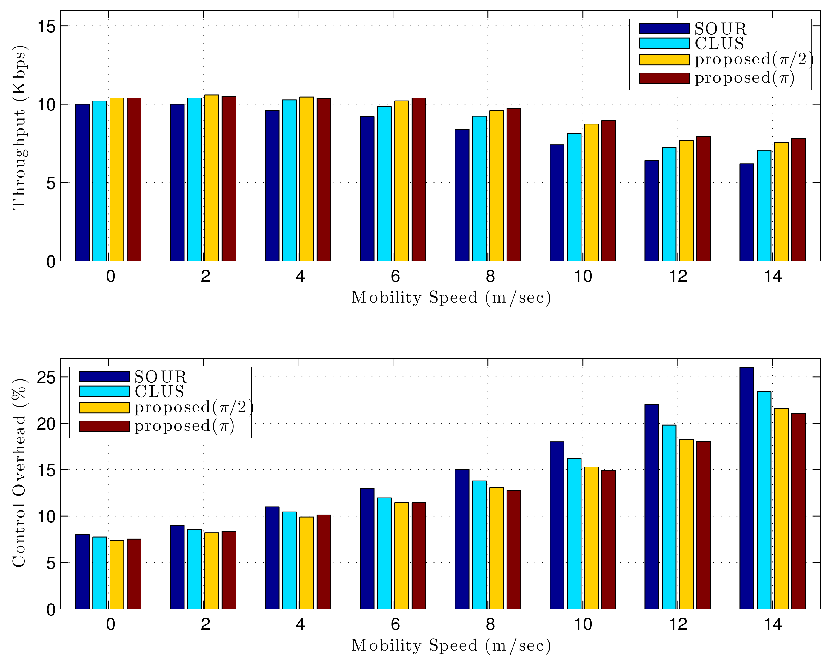
Figure 6 shows the performance when the network size was 1 km × 1 km. Figure 6 compares the throughput, showing how many data packets could be sent successfully from the source to the destination. The proposed control exploits redundant paths as backup links or relayed cooperative links. Backup links increase the throughput by reducing the time for link recovery, and relayed cooperative links can increase throughput by sending the same information at the same time to enhance the signal-to-noise ratio. In contrast, in SOUR and CLUS, information is sent along a single path based on a noncooperative mode. Comparing SOUR and CLUS, the proposed control provided $26\%$ and $12\%$ enhanced throughput. Figure 6 also compares the control packet overhead to successfully deliver data traffic from the source to the destination. Control packet overhead is strongly related to transmission-path management tasks such as finding new routes and recovering from link failures. The proposed approach reduced the control packets using predetermined stable hub paths and redundant local paths, minimizing frequent route discovery processes. It also used simpler maintenance messages—i.e., HelloHub and ByeHub messages. In contrast, in SOUR, the intermediate node started the source routing whenever there was a link failure. Frequent route-retrieval processes that rely on network-wide flooding mechanisms increase control overhead. The CLUS had higher overhead because of its complex cluster and gateway selection mechanism and various cluster head and gateway messages. Comparing SOUR and CLUS, the proposed control gave $19\%$ and $9\%$ lower overhead. On the other hand, in a low mobility environment, the proposed ($\pi$) gave a higher performance than the proposed ($\pi /2$). However, as the movement speed increased, the proposed ($\pi /2$) gave a better performance than the proposed ($\pi$), because the number of synchronized nodes is more important than the synchronization strength in the slow movement, and the synchronization strength is more important than the number of synchronized nodes in the fast movement. The larger is $\theta$, the greater is the number of synchronized nodes, but the weaker is the synchronization. Figure 7 shows the performance when the network size was 2 km × 2 km. Comparing SOUR and CLUS, the proposed control gave $32\%$ and $15\%$ enhanced throughput, and $34\%$ and $13\%$ reduced overhead. From these simulations, we can see that the performance gain increased as the network size grew larger.

6. Conclusions

In this paper, we propose a distributed and localized hub based on a hierarchical transmission-control scheme for large-scale wireless networks. The proposed control consists of macroscopic and local transmission controls. For the macroscopic control, we exploit stable nodes with low mobility to construct a virtual hub infrastructure that can stochastically support stochastic end-to-end delay constraints. We also suggest a stochastic integer programming model and virtual flooding-based heuristic search algorithm capable of providing high-performing hub transmission paths. For the local control, we suggest a way to establish redundant local transmission paths between hubs and a way to use the redundant links as backup links, relays, or cooperative links. Simulation confirmed that the proposed hierarchical control had higher throughput and more reduced control overhead than SOUR and CLUS. The proposed control became more efficient as the wireless network became larger. As a future work, we will extend the proposed algorithm as follows: (1) by combining it with machine learning for local hub selection; (2) by applying service-related practical simulation parameters; (3) by applying distribution that is better suited to real-world situations; (4) by designing stable data transmission for large-scale sensor networks with low energy; and (5) by implementing in NS-3.

References

1. Mishra, A. Security and Quality of Service in AdHoc Wireless Networks; Cambridge University Press: New York, NY, USA, 2008. [Google Scholar]
2. Tao, M.; Yuan, H.; Wei, W.; Li, Z.; Qin, Y. Geographic Information Assisted Routing Flexibility Control in Hierarchical AdHoc Networks. In Proceedings of the Chinese Control Conference (CCC’13), Xi’an, China, 26–28 July 2013. [Google Scholar]
3. Zhang, X.; Xu, C.; Xu, J. Hierarchical ZRP’s Performance vs. ZRP’s Performance in MANET. In Proceedings of the IEEE International Conference on Communication Software and Networks (ICCSN’15), Chengdu, China, 6–7 June 2015. [Google Scholar]
4. Asadinia, S.; Rsfsanjani, M.K.; Saeid, A.B. A Novel Routing Algorithm Based on an Ant Colony in Mobile AdHoc Networks. In Proceedings of the IEEE International Conference on Ubi-Media Computing (U-Media’10), Jinhua, China, 5–6 July 2010. [Google Scholar]
5. Derenick, J.; Thorne, C.; Spletzer, J. On the Deployment of a Hybrid Free-Space Optic/Radio Frequency (FSO/RF) Mobile AdHoc Network. In Proceedings of the IEEE/RSJ International Conference on Intelligent Robots and Systems, Edmonton, AB, Canada, 2–6 August 2005. [Google Scholar]
6. Agarwa, S.; Rishiwal, V.; Arya, K.V. Fallout of Different Routing Structures for Different Mobility Patterns in Large AdHoc Networks. In Proceedings of the Confluence 2013: The Next Generation Information Technology Summit, Noida, India, 26–27 September 2013. [Google Scholar]
7. Venkatesan, T.; Rajakumar, P.; Pitchaikkannu, A. Overview of Proactive Routing Protocols in MANET. In Proceedings of the 4th International Conference on Communication Systems and Network Technologies (CSNT’14), Bhopal, India, 7–9 April 2014. [Google Scholar]
8. Das, B.; Bharghavan, V. Routing in AdHoc Networks Using Minimum Connected Dominating Sets. In Proceedings of the IEEE International Conference on Communications (ICC ’97), Montréal, QC, Canada, 8–12 June 1997. [Google Scholar]
9. Yang, Q.; Nofsinger, A.; McPeek, J.; Phinney, J.; Knuesel, R. A Complete Solution to the Set Covering Problem. In Proceedings of the International Conference on Scientific Computing (ICSC ’15), Firenze, Italy, 16–24 May 2015. [Google Scholar]
10. Coelho, R.; Moura, P.; Wakabayashi, Y. The K-Hop Connected Dominating Set Problem: Approximation and Hardness. J. Comb. Optim. 2017, 34, 1060–1083. [Google Scholar] [CrossRef]
11. Birge, J.; Louveaux, F. Introduction to Stochastic Programming, 2nd ed.; Springer: Berlin, Germany, 2011. [Google Scholar]
12. Sukhov, A.; Kuznetsova, N. What Type of Distribution for Packet Delay in a Global Network Should Be Used in the Control Theory? arXiv 2009, arXiv:0907.4468v1. [Google Scholar]
13. Coluccia, A.; Ricciato, F. On the Estimation of Link Delay Distributions by Cumulant-based Moment Matching. Internet Technol. Lett. 2018. [Google Scholar] [CrossRef] [Green Version]
14. Patel, M.K.; Berber, S.M.; Sowerby, K.W. Maximal Ratio Combining Using Channel Estimation in Chaos Based Pilot-Added DS-CDMA System with Antenna Diversity. Wirel. Commun. Mob. Comput. 2017, 2017, 3607167. [Google Scholar] [CrossRef]
15. Iyer, B.; Nalbalwar, S.L.; Pathak, N.P. Communication and Signal Processing; Springer: Singapore, 2018. [Google Scholar]
16. MATLAB Toolbox R2018. Available online: https://www.mathworks.com (accessed on 1 October 2019).
17. Salem, A.; Samara, G.; Alhmiedat, T. Performance Analysis of Dynamic Source Routing Protocol. J. Emerg. Trends Comput. Inf. Sci. 2014, 5, 97–100. [Google Scholar]
18. Rezaee, M.; Yaghmaee, M. Cluster-based Routing Protocol for Mobile adhoc Networks. INFOCOMP J. Comput. Sci. 2009, 8, 30–36. [Google Scholar]
Figure 1. System model.
Applsci 09 05283 g001
Figure 2. Synchronization.
Applsci 09 05283 g002
Figure 3. Local Route Setup Procedure.
Applsci 09 05283 g003
Figure 4. Local route reply procedure.
Applsci 09 05283 g004
Figure 5. Local route establishment procedure.
Applsci 09 05283 g005
Figure 6. Networks size: 1 km × 1 km.
Applsci 09 05283 g006
Figure 7. Networks size: 2 km × 2 km.
Applsci 09 05283 g007