Article

Evaluation of Skin Friction Drag Reduction in the Turbulent Boundary Layer Using Riblets †

1
Research and Development Directorate, Japan Aerospace Exploration Agency, Kakuda, Miyagi 981-1525, Japan
2
Aeronautical Technology Directorate, Japan Aerospace Exploration Agency, Chofu, Tokyo 182-8522, Japan
*
Author to whom correspondence should be addressed.
This paper is an extended version of paper published in 56th Aerospace Sciences Meeting (AIAA SciTech 2018), Kissimmee, FL, Florida, USA, 8–12 January 2018. Paper No.: AIAA-2018-0839.
Appl. Sci. 2019, 9(23), 5199; https://doi.org/10.3390/app9235199
Submission received: 10 October 2019 / Revised: 27 November 2019 / Accepted: 27 November 2019 / Published: 29 November 2019
(This article belongs to the Section Mechanical Engineering)

Abstract

:
A unique approach to evaluate the reduction of skin friction drag by riblets was applied to boundary layer profiles measured in wind tunnel experiments. The proposed approach emphasized the turbulent scales based on hot-wire anemometry data obtained at a sampling frequency of 20 kHz in the turbulent boundary layer to evaluate the skin friction drag reduction. Three-dimensional riblet surfaces were fabricated using aviation paint and were applied to a flat-plate model surface. The turbulent statistics, such as the turbulent scales and intensities, in the boundary layer were identified based on the freestream velocity data obtained from the hot-wire anemometry. Those turbulent statistics obtained for the riblet surface were compared to those obtained for a smooth flat plate without riblets. Results indicated that the riblet surface increased the integral scales and decreased the turbulence intensity, which indicated that the turbulent structure became favorable for reducing skin friction drag. The proposed method showed that the current three-dimensional riblet surface reduced skin friction drag by about 2.8% at a chord length of 67% downstream of the model’s leading edge and at a freestream velocity of 41.7 m/s (Mach 0.12). This result is consistent with that obtained by the momentum integration method based on the pitot-rake measurement, which provided a reference dataset of the boundary layer profile.

1. Introduction

More and more people are traveling by air, so the demand for economical and environmentally friendly aircraft is also increasing. Meeting these needs will require improvements in aerodynamic efficiency and in reduced drag. In addition, these goals must be met while addressing environmental concerns, such as reducing carbon dioxide emissions to help combat global warming. Since skin friction drag constitutes over half of the total drag on an aircraft [1], reducing it is key to both increasing aerodynamic performance and reducing fuel consumption.
Riblets are one of the methods used to reduce aircraft surface drag [1,2,3,4]. They are a passive means of turbulent flow control near the wall and were first used by the NASA Langley Research Center in the 1970s [3,5]. They imitate the fine structure of the skin of a shark, which is known for being able to swim long distances at high speed. Riblets are fine grooves aligned in the direction of a flow across a surface that induce a streamwise vortex, which reduces the turbulent flow in a boundary layer that causes surface drag, thus reducing skin friction drag.
To date, much research has studied the mechanism [3,4,5,6] and effectiveness [7] of riblets in reducing skin friction drag, with many industrial applications to wind turbine blades, railways, and aircraft [8]. These studies have clarified a number of design criteria, such as the height, width, and skewness of the peak shape of the riblets in reducing skin friction drag for flowfields of interest. The 3M company has demonstrated riblets that reduced skin friction drag by 4% to 6% over the flowfield with no pressure gradients or zero incidence [8]. With the aid of computer simulation and high-resolution measurements, riblets can reduce skin friction drag by 10% by optimizing the geometry of the riblets for the flowfield [9,10,11,12]. The Airbus company has conducted wind tunnel tests with riblets attached to an entire airframe surface and has demonstrated a reduction in skin friction drag of 2% [1,13]. According to an estimate by the Airbus company, even a 1% drag reduction can reduce annual operating costs by more than a million dollars per aircraft [1,13]. Therefore, reducing skin friction drag has a significant economic impact [4].
To improve the drag-reducing performance further, multi-dimensional riblet shapes, such as two-dimensional ‘blade riblets’, which aligned a row of thin fences along the streamwise direction [12], and three-dimensional zigzag riblets [14], and sinusoidal riblets [9,14,15,16,17], have emerged. Among those intensive past studies, three-dimensional sinusoidal riblets [9,14,15,16,17] are found to be more effective compared to conventional straight-shaped riblets. Grüneberger et al. [14] investigated the influence of wavelengths and amplitudes of sinusoidal riblets on the effectiveness of drag-reducing performance and concluded that certain combinations of a height/spacing ratio can improve drag reduction. However, the drag-reducing performance by the straight-shaped riblets could become comparable once the geometry of the riblet grooves aligned to the streamwise direction is optimized for the flowfield of interest. Additionally, three-dimensional riblet shapes may cause adverse pressure gradients, which results in the benefit of drag-reducing ability being suppressed by inducing additional turbulence in the boundary layer. Peet et al. [17] addressed the design criteria for three-dimensional sinusoidal riblets with respect to their amplitude and wavelength and showed that approximately a 2% drag-reduction improvement can be expected over a conventional straight-shaped riblet. Thus, three-dimensional riblets with well-designed geometry for a flowfield of interest are considered to be effective for the reduction of skin friction drag.
When considering the use of riblets on an aircraft, it is necessary to consider fabrication costs, maintainability, and sustainability through changes in the environment where they are exposed, while maintaining aircraft performance. It is also necessary to optimize riblet design according to their locations on the aircraft (e.g., fuselage, wing, etc.), and for any changes in flight conditions and attitude. To this end, it is vital to investigate how riblets affect boundary layer flowfields and to explore useful fabrication techniques. The Japan Aerospace Exploration Agency (JAXA) has been investigating the effectiveness of riblets to reduce skin friction drag [18,19] as part of their environmentally friendly aircraft research project: Flight Investigation of skiN-friction reducing Eco-coating (FINE). The riblet study aims to develop riblets fabricated by using aviation paint and to demonstrate their drag-reducing capability by flight tests.
Since many insights on the use of riblets for reducing skin friction drag have been revealed as mentioned above, this study focused on exploring a new evaluation approach for the reduction of skin friction drag. The primary objective of this study was to propose a unique method to evaluate the reduction of skin friction drag by emphasizing the turbulent length scales.
To this end, the riblet designed by the JAXA’s FINE project was employed as a reference riblet in wind tunnel experiments to obtain boundary layer characteristics being altered from those of a flat smooth surface. Note that the geometry optimization of riblets is not a scope of this study since this study focused on the applicability of the proposed method to evaluate the reduction of skin friction drag. Hot-wire anemometry was used for primary data acquisition since the technique offers high-resolution rapid measurements. By using the detected signals from the hot-wire probe, signal processing and statistical autocorrelation analysis were employed to evaluate the reduction of skin friction drag. The method compared the riblet surface to the smooth surface without riblets. Another benefit of using hot-wire anemometry is that it may reduce uncertainty inherent in the experiment since less equipment is required than in optical diagnostics [20,21], pitot-rake measurements, or cantilever experiments [22,23]. The signal was temperature corrected to convert the raw output voltage [24] to quantitative freestream velocity (U velocity). Based on the U velocity data obtained by the hot-wire anemometry, the reduction of skin friction drag was evaluated by relating the skin friction drag coefficient with turbulent scales derived from statistical analysis. The turbulent boundary layer profile obtained with the riblet surface was compared to that obtained with a smooth flat plate surface.

2. Wind Tunnel Apparatus, Equipment, and Test Conditions

2.1. Wind Tunnel Facility

Wind tunnel experiments were carried out by using the low-turbulence wind tunnel facility managed by the JAXA Chofu Aerospace Center in Tokyo. It is a closed-circuit wind tunnel, which offers a running time of multiples of at least 10 minutes. The flow speed can be altered continuously while running the wind tunnel in the range of 10 to 80 m/s. The turbulence level in the freestream at the exit of the wind tunnel nozzle is 0.05% at the freestream velocity of 30 m/s. Figure 1 illustrates a schematic of a test model installed at the center of the wind tunnel duct. The test section has a rectangular cross section that is 0.65 m high, 0.55 m wide, and 1.5 m long. The coordinates and the origin are also shown in Figure 1.

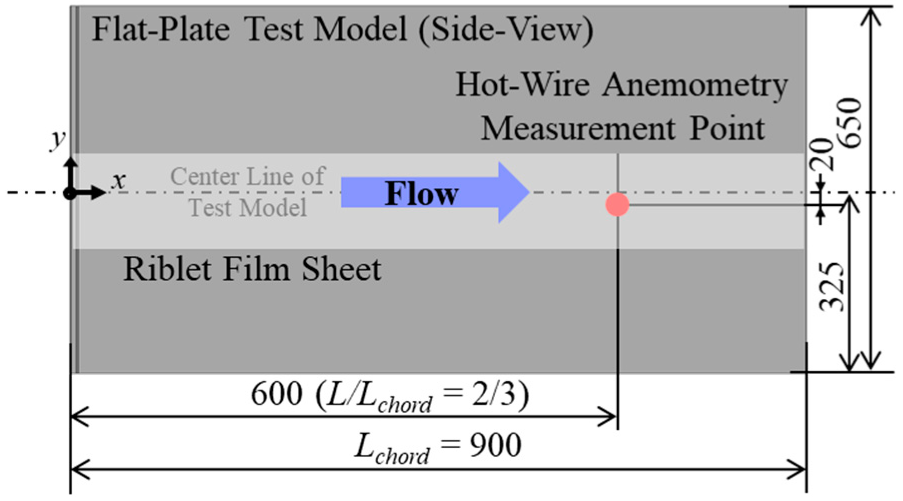
2.2. Flat-Plate Model
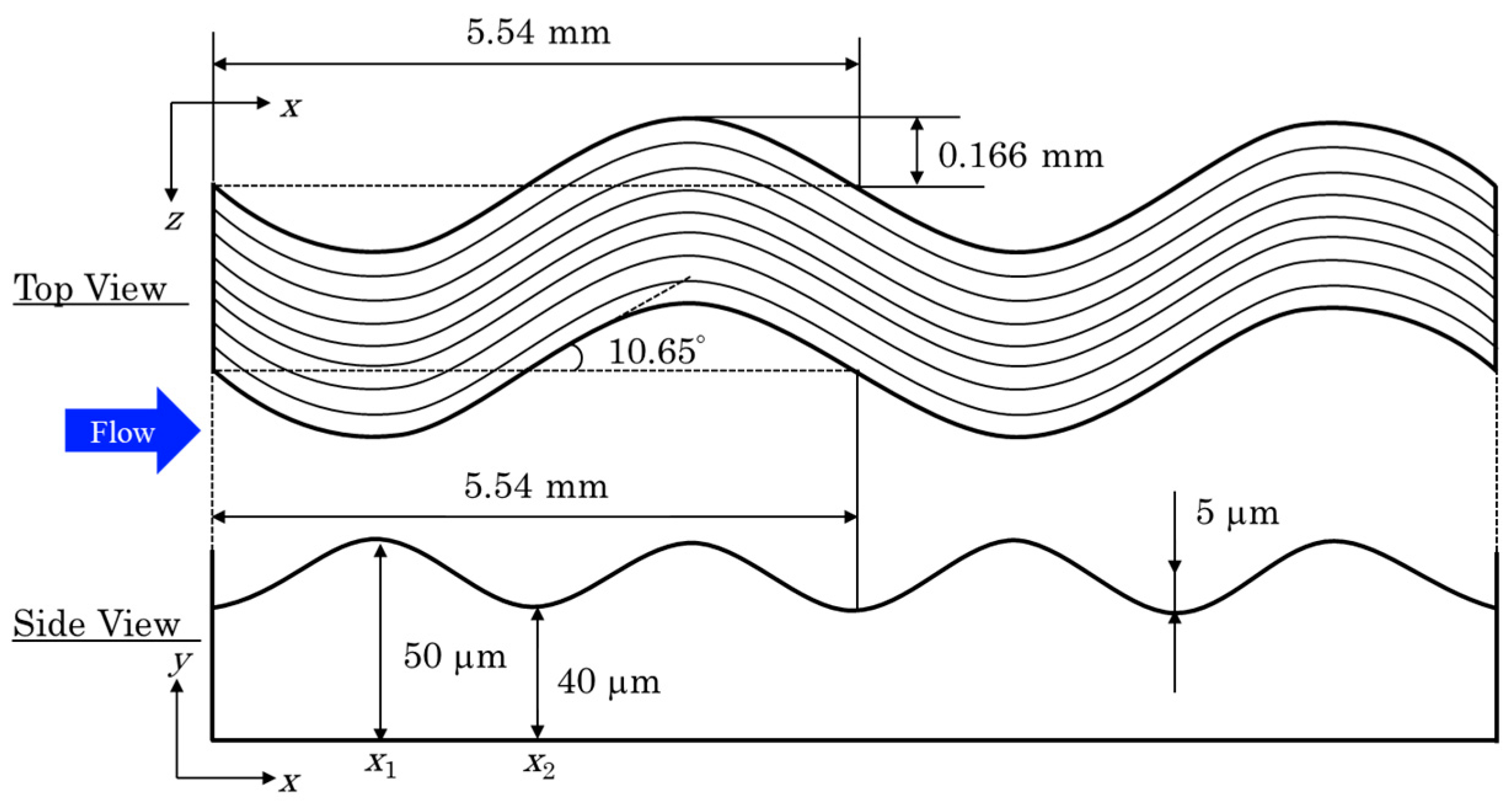
During the tests, a riblet surface attached to the surface of a flat aluminum plate was investigated. The setup of the flat-plate model, which had an effective span length of 650 mm, a chord length of 900 mm, and a thickness of 10.8 mm, is shown in Figure 1. An array of disk-shaped roughness elements (a product of CAD-CUT Inc.) were used, each element being 0.29 mm high with a diameter of 1 mm. The array was attached to the test model surface 20 mm downstream of the leading edge at intervals of 2.54 mm in the spanwise direction. The location from the leading edge (x = 20 mm) where the disk roughness was located will be referred to as a virtual origin in the evaluation process of the reduction of skin friction drag in a later section. The disk roughness was used to trip the boundary layer. The roughness height was determined to be 50% of the assumed laminar boundary layer thickness, given by δ l a m i n a r ( x ) 5.0 x R e x 1 / 2 [25].
Figure 2 shows the details of the leading edge of the flat-plate model. The effect of the shape of the leading edge on the evolution of the boundary layer profile is discussed later in this section.
Figure 3 shows the shape factor (H12), which is the ratio between the displacement thickness (δ**) and the momentum thickness (θ), at several stations from the leading edge measured by using the pitot-rake (described in a later section). The displacement thickness and the momentum thickness are expressed in Equation (1) and Equation (2), respectively. Those values were based on the velocity profile in the boundary layer measured by pitot rake. The shape factor (H12) is also expressed as Equation (3) and was used to evaluate the flow state in the boundary layer. In general, in the turbulent boundary layer, the higher that H12 is, the stronger the adverse pressure gradient. The value of H12 would typically be 1.3 to 1.4 for a fully developed turbulent boundary layer:
δ * = 0 ( 1 U ( z ) U ) d z ,
θ =   0 U ( z ) U ( 1 U ( z ) U ) d z ,
H 12 = D i s p l a c e m e n t   T h i c k n e s s M o m e n t u m   T h i c k n e s s = δ * θ .
In Figure 3, the horizontal axis is the Reynolds number based on the measurement location from the leading edge and the freestream velocity. Three plots obtained at three different measurement locations (x/xchord = 1/2, 2/3, and 0.94 or x = 450, 600, and 850 mm, respectively) are plotted for comparison. As seen in Figure 3, H12 lies approximately 1.4 for a Reynolds number range of 6.0 × 10⁵ to 4.0 × 10⁶, which corresponds to a freestream velocity range of 25 to 80 m/s downstream 450 mm (x/xchord = 1/2). Therefore, the primary measurement using the hot-wire anemometry was implemented at x = 600 mm (x/xchord = 2/3) from the leading edge.

2.3. Riblets

The riblet surface was fabricated from an aviation paint-based material and was designed by the JAXA’s FINE project. The paint-based riblet had a three-dimensional sinusoidal structure with V-grooves aligned in the streamwise direction and were fabricated on an aviation surface sticker. The top-view and side-view configurations of the riblet are presented in the upper and lower figures, respectively, in Figure 4. The riblet geometry had a width (s) of 200 μm, height (h) of 40 to 50 μm, and a spacing of 200 μm. More details on the design of the riblet geometry can be found in another precursor study [9]. A flat sheet sticker 90 to 100 mm wide where the riblet was fabricated was attached to the flat plate test model surface to provide the riblet surface as illustrated in Figure 1.

2.4. Test Conditions

One of the governing parameters was considered to be the freestream velocity (U velocity) since it is important to determine the wind tunnel freestream velocity accurately so that the boundary layer has already transited from laminar to turbulent and is marginally in the turbulent state at measurement points. Moreover, it is desirable to be in the range where the skin friction-reducing effect is likely to appear. In this sense, the test condition was determined by one of the most effective parameters for evaluating the skin friction drag: The nondimensional width of the riblet, s+, which is expressed by Equation (4):
s + = s · u τ v ,
u τ = τ 0 ρ ,
τ 0 = c f · ( 1 2 ρ U 2 ) ,
c f = 0.059 · R e x 1 5 ,
where ν is the kinematic viscosity, the value of which at the test condition was found to be 1.57 × 10⁻⁵ m2/s assuming that the total and static temperatures of the freestream are the same because the flow was incompressible, and that the measured total temperature of the freestream was 30 °C. The value of s+ under these conditions was 17, where the riblet’s effect would be dominant if the boundary layer had become turbulent [26]. Other variables used to calculate for s+ are the friction velocity (uτ), Reynolds stress (τ0), and local skin friction coefficient (cf) expressed in Equations (5)–(7) [27], respectively. Note that the Reynolds stress (τ0) is physically equivalent to the skin friction drag. The actual freestream velocity ( U ¯ ) was in the range of 40 to 75 m/s, determined from a pitot-tube measurement carried out separately. In this study, the freestream velocity was fixed at 41.7 m/s or Mach 0.12. The freestream Reynolds number at x = 600 mm (x/xchord = 2/3), where the hot-wire probe and the pitot-rake would be placed, was 1.6 × 10⁶. Accounting for the Reynolds number value and the observation from Figure 3, the boundary layer was considered to be fully turbulent at this measurement location. The nondimensional height of the riblet ranges between 3.40 and 4.25, which were calculated by Equation (4) with the riblet heights described in the previous section.

3. Measurement Technique and Data Reduction Methodologies

This section presents measurement techniques of hot-wire anemometry and pitot-rake measurement, and data reduction methodologies used to derive the turbulent properties and to evaluate the reduction of skin friction drag.

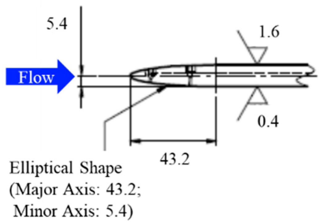
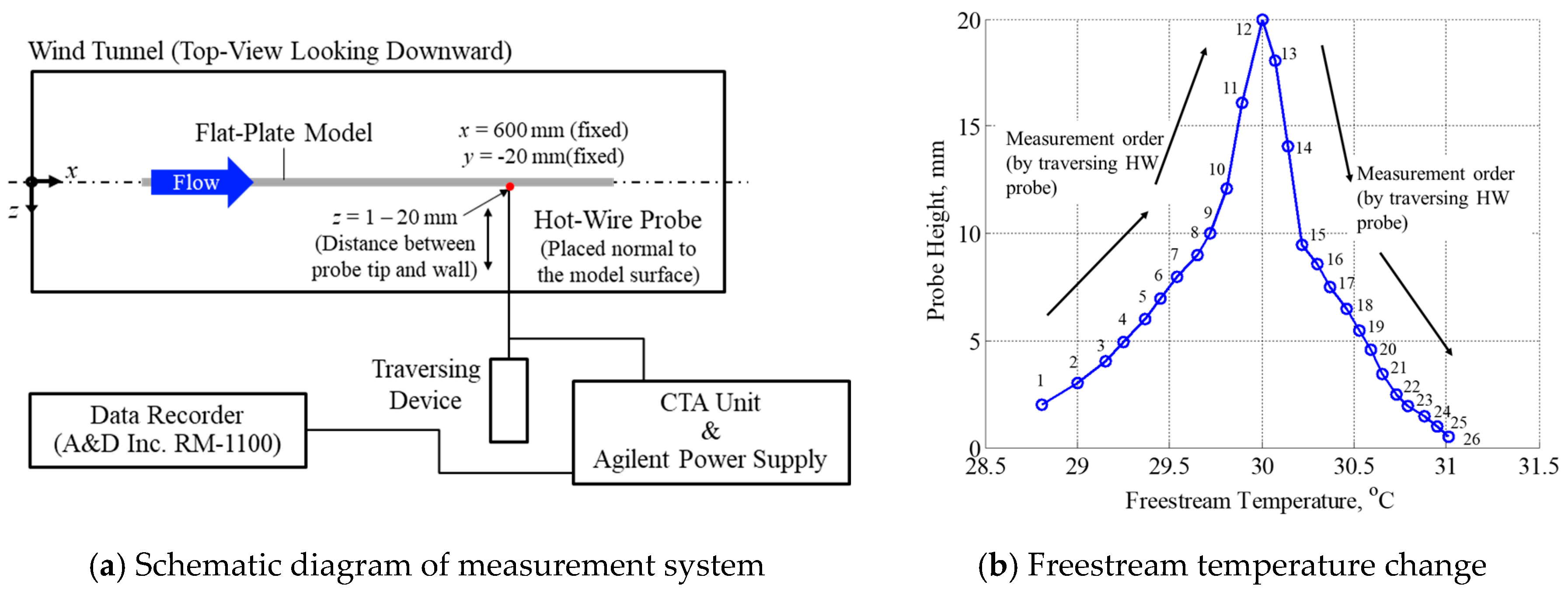
3.1. Hot-Wire Anemometry

Hot-wire (HW) anemometry was used to extract the turbulent structure statistically inherent in the unsteady random flow process because it offers high-resolution measurements, both temporally and spatially, with a high frequency response. A standard single hot-wire probe made of Tungsten (KANOMAX Inc., 0251R-T5) was employed. The wire had a diameter of 5 μm and was 2 mm long. The prong length was 7 mm.
The signal detected by the hot wire, equivalent to the flow velocity, was converted to a voltage by an A/D converter (KANOMAX Inc., constant temperature hot-wire anemometer: CTA). The voltage data were acquired by a data recorder (A&D Inc., RM-1100) at a sampling frequency (f) of 20 kHz. Data acquisition was carried out for more than 30 s at every measurement location; of the 30-s measurements, 5-s data was used to capture a boundary layer profile and 15-s data at each measurement location was used for turbulent analysis. This duration was considered to be long enough to extract the turbulent statistical feature as the characteristic frequency of the flowfield would be in the order of 1 kHz or 1 millisecond, and therefore more than 10,000 samples of characteristic turbulent feature data were expected to be acquired from each dataset.
Measurement locations were x = 600 mm (x/xchord = 2/3) and y = –20 mm (y/ywidth = –0.031), as shown in Figure 5a presenting a schematic diagram of the measurement system; the probe position in the z-direction was only varied by using an electrically controlled traversing system. Total measurement locations with respect to the z position were 26, where the z position was varied from 1 to 20 mm from the wall surface. The uncertainty in positioning the z location was determined from the relationship between the read count of the stepping motor of the traversing system and the actual traversed distance. The probe height at each wind tunnel run was checked to be firmly fixed by reading the read count during each wind tunnel operation. The uncertainty for positioning was found to be negligible. The vertical position was changed, starting from z = 2.0 to 10 mm, which is around the upper edge of the boundary layer, with an increment of 0.5 mm. It was then increased by increments of 2 or 4 mm until it reached z = 20 mm. After the measurement at z = 20 mm, the height was changed in the other direction (in the order of decreasing height) to check for hysteresis.
Figure 5b plots a representative freestream temperature change for the smooth wall configuration during a wind tunnel operation with changing of the probe position (i.e., z position). The sequential numbers on the figure indicate the order of measurement: The larger the number, the longer the wind tunnel operation time is. Obviously, the freestream temperature increases gradually as the wind tunnel operation becomes longer. Not shown here but a similar observation of large temperature variation was seen in each wind tunnel run. Because the resistance of the hot-wire probe is a function of flow properties, such as freestream velocity and temperature, an appropriate temperature correction must be made in the post-process for quantitative analysis. The details of the temperature correction will be described later.
The same hot-wire probe was used for measurements for both the smooth and riblet walls in order to eliminate any uncertainty due to differences between probes. Additionally, the condition of the probe was checked by measuring its resistance and also by visual inspection. The resistance was around 4.0 Ω before and after testing and the absence of damage to the probe was confirmed. Another fact that should be accounted for is that the tungsten probe may involve a time decay in its output under long-duration measurements where temperature changes of freestream are involved. A slight time decay in the output signal was seen during the experiments, but the decay could be translated into velocity data properly by the temperature correction method, which will be described later.
The orientation of the probe stem relative to the test surface is also important because the probe assembly can affect the extent of boundary layer disturbance. The probe orientation relative to the freestream was fixed so that the probe wire was perpendicular to the flow; the stem is also normal to the wall surface. Since the hot-wire probe is perpendicular to the flow, the streamwise component of the flow is considered to be the most sensitive, and hence the measured velocity was taken as the U velocity. Note that the uncertainty that may be inherent in the flow measurement caused by the spanwise and vertical velocity components will be discussed in a later section along with other uncertainty analysis. Based on the measured U velocity and resulting turbulent scales in their horizontal component, the reduction of skin friction drag will be evaluated.
The reference height for the smooth wall was z = 0 mm and that for the riblet wall was z = 50 μm where the riblet peak appeared at the measurement point. The same reference heights were used for the pitot-rake measurement as well.

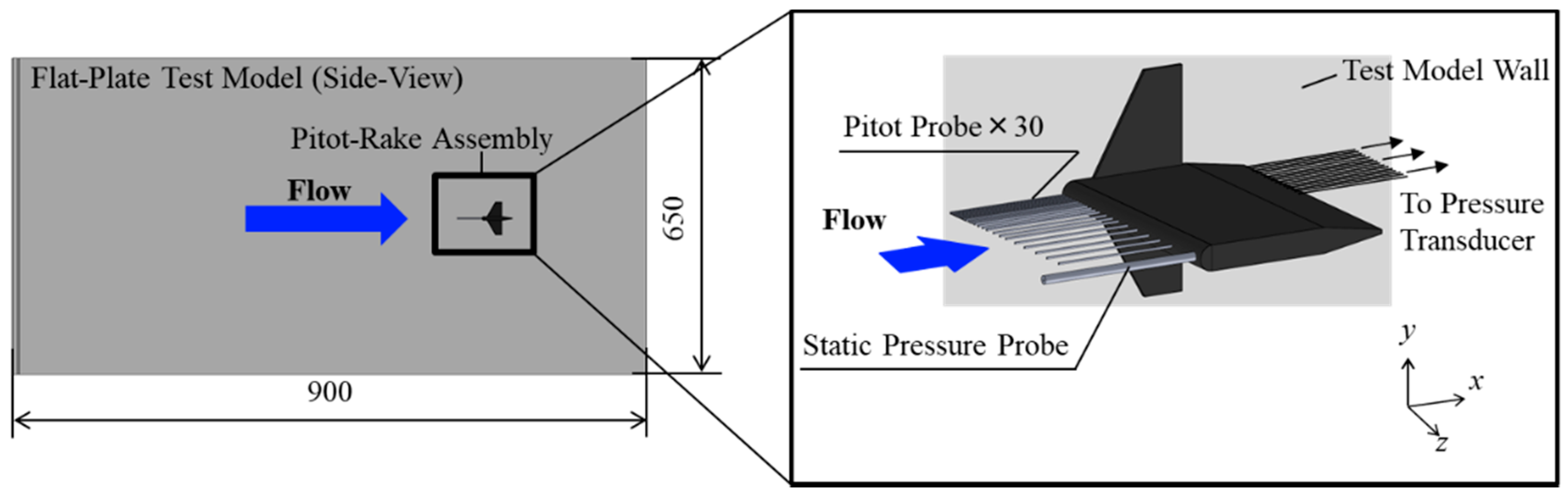
3.2. Pitot-Rake Measurement

Pitot-rake measurement was done in order to validate the boundary layer profile established by hot-wire anemometry since the pitot-rake measurement for this kind of simple incompressible flowfield is adequately robust to measure the boundary layer profile via high-accuracy pressure transducers. Figure 6 is a schematic illustration showing the pitot-rake assembly attached to the flat-plate test model surface. There are 30 probes with an outer diameter of 0.5 mm, an inner diameter of 0.3 mm, and a length of 30 mm. A static pressure probe is also attached outside most of the probes. The boundary layer characteristics, including its profile, momentum thickness, displacement thickness, and shape factor, were evaluated by the aforementioned equations. Note that those values were also used to assure that the measured boundary layer profile by the hot-wire anemometry was appropriate by comparing it with those by pitot-rake measurements.

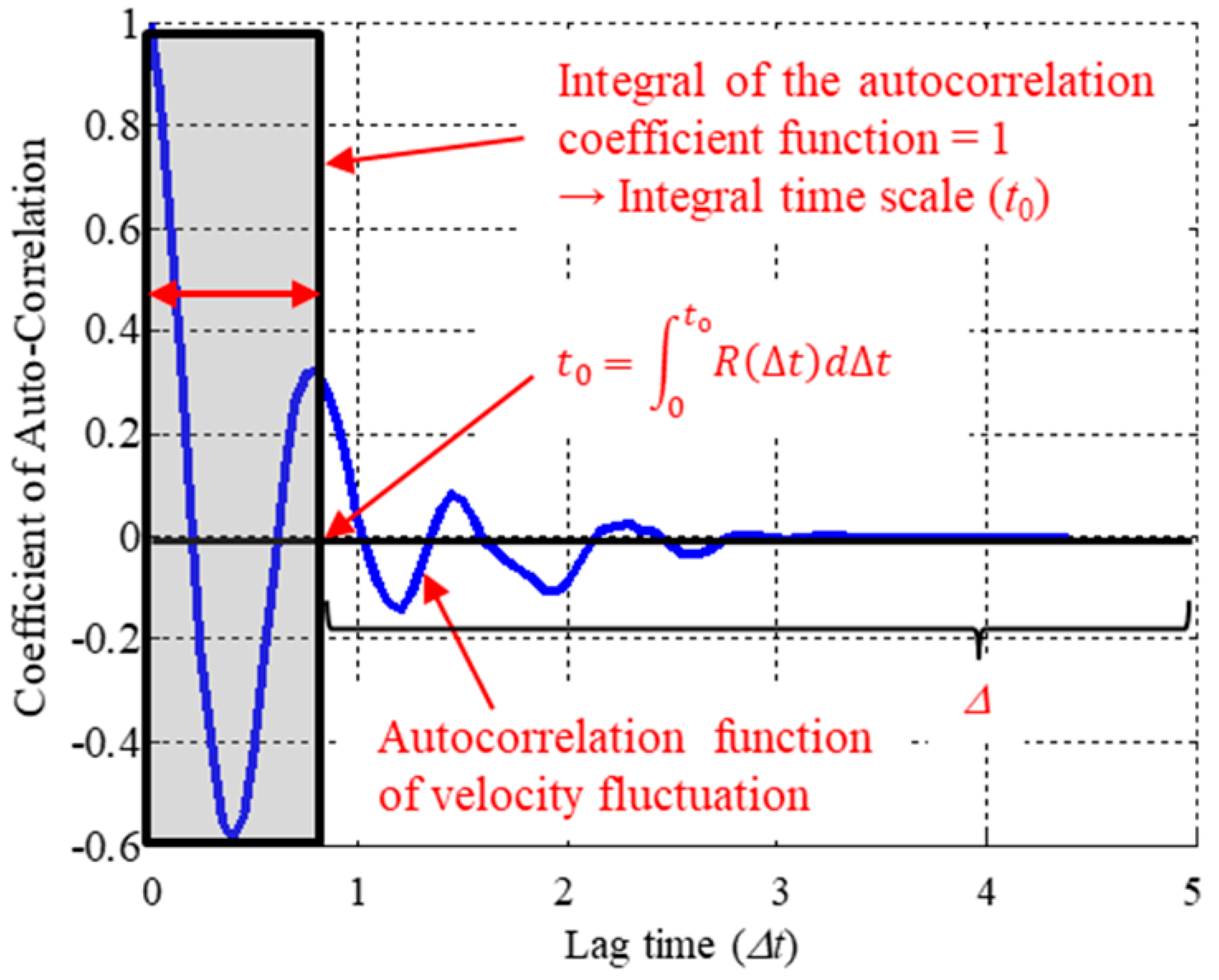
3.3. Integral Time and Length Scales

This section describes the procedures for deriving the integral time and length scales, which represent the statistically largest-scale vortex structure containing most of the energy of the flow. The integral time and length scales were derived by the following procedure based on the autocorrelation for the fluctuating component of the U velocity.
(i) Measured U velocity was decomposed into its mean component ( U ¯ ) and its fluctuating component (u’) by the use of the Reynolds decomposition expressed by Equation (8):
U = U ¯ + u .
(ii) The autocorrelation coefficient (R) for the fluctuating component of the time-series output signal ( u = U U ¯ ) with data length of N was calculated using Equation (9). The autocorrelation coefficient can be plotted against the lag time (Δt) as illustrated in Figure 7:
R ( Δ t ) = i = 1 N m ( U i U ¯ ) ( U i + m U ¯ ) i = 1 N ( U i U ¯ ) 2 ;   Δ t = m / f .
(iii) By taking the integral for the autocorrelation coefficient function and using Equation (10) [28] for 0 ~ Δt s, a certain Δt value, which becomes equal to the integrated autocorrelation function value, can be found. The resulting Δt is the integral time scale (t0). This procedure for computing t0 is illustrated in Figure 7. Here, the integration from 0 to t0 (the first term in the right side in Equation (10)) was only considered to have a significant value and the integration from t0 to infinity (the second term in the right side in Equation (10)) was considered to have a negligible effect on the integration of the autocorrelation function. Thus, the latter was truncated and was considered to be an uncertainty. This also helps to reduce uncertainty when integrating to infinity since the upper limit of the integration depends on the acquired data length. The derived integral time scale corresponds to the largest time scale of turbulence and represents the largest scale of the flow structure that contains most of the energy in the energy cascade process where the Kolmogorov’s –5/3 log-law can be applied. This definition is a general definition to identify the integral time scale, and therefore was used in this study. For calculating the integral, various methods, such as curve fitting for a complex integral profile, can be applied. In this analysis, the MATLAB interpolation function was used with a time interval of 0.1Δt (= 5 μs), so the uncertainty inherent in this integration was considered to be up to 0.1Δt. This uncertainty was also considered to include the uncertainty resulting from the aforementioned tiny amounts Δ that appeared in Equation (10):
t 0 = 0 R ( Δ t ) d Δ t = 0 t 0 R ( Δ t ) d Δ t + t 0 R ( Δ t ) d Δ t = 0 t 0 R ( Δ t ) d Δ t + Δ .
By multiplying the integral time scale (t0) and mean velocity ( U ¯ ) together under Taylor’s hypothesis of frozen turbulence (Equation (11)), the turbulent length scale (L0) was obtained as expressed in Equation (12):
t = | U | x ,
L 0 = U ¯ · t 0 .
Here, Taylor’s hypothesis is generally applicable when the flow condition is u / U ¯ 1 ; the value for the smooth wall, for example, was 0.011 at maximum, and therefore, it is plausible that Taylor’s hypothesis is applicable to the current measurement. The length (L0) is the integral length scale that determines the largest turbulent scale inherent in the flow region of interest.

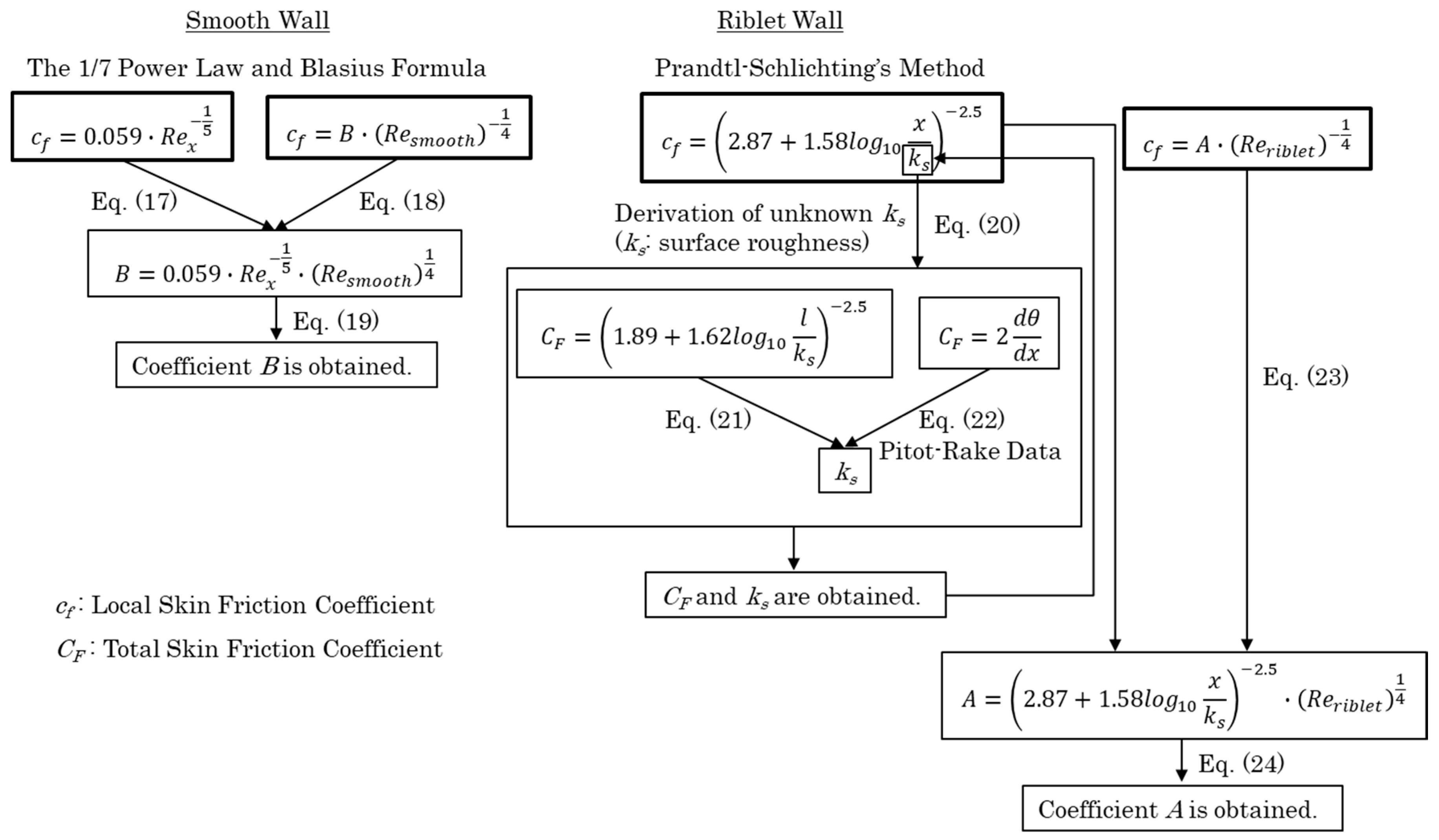
3.4. Evaluation of Skin Friction Drag Reduction

The effect of reducing skin friction drag was evaluated by Equation (13), which accounts for a ratio between the difference of the local skin friction coefficient (Δcf) between the riblet and smooth wall cases and the reference value for the smooth wall:
Δ c f c f ,   s m o o t h = c f ,   r i b l e t c f ,   s m o o t h c f ,   s m o o t h .
In general, the local skin friction coefficient in the turbulent boundary layer for a smooth flat plate surface with zero incidence can be calculated by Equation (7). However, the local skin friction coefficient for the riblet surface (cf,riblet) cannot be calculated properly by Equation (7) since the constant coefficient value may be different. To evaluate the local skin friction coefficient in case for the riblet surface, a unique approach was proposed here by emphasizing the turbulent Reynolds number and the turbulent scale. The detailed procedure for the evaluation is given in this section.
The procedure for calculating Δcf is described here in more detail. The local skin friction was basically calculated based on the turbulent boundary layer theory and the 1/7 power law applied to a flat smooth plate based on the Blasius formula [29] as presented by Equation (14). Note that this equation is equivalent to Equation (7) in case for a flat smooth plate:
c f = τ 0 1 2 ρ U ¯ 2 = C · ( U ¯ · δ v ) 1 4 ,
where C is a constant coefficient, which is usually 0.045 for a smooth flat plate. This value may be different for different surface conditions as aforementioned; since the actual value for the riblet surface is unknown, a simple estimate of this parameter will be given; details will be given later in this section. The value of the parenthesized quantities on the right side of Equation (14) was equivalent to the turbulent Reynolds number (Returb), given by Equation (15). Here, it was assumed that the integral length scale (L0) generally increases to the boundary layer thickness (δ), and the boundary layer thickness increases as the flow proceeds downstream. Therefore, the integral length scale was considered to grow with movement downstream. Additionally, the characteristic velocity scale was considered to be the root-mean-square velocity (σu) to focus on the turbulent characteristics of the boundary layer flow. Thus, the turbulent Reynolds number was calculated based on the integral length scale and the root-mean-square velocity. This relationship emphasizes the relation between the turbulent structure and the skin friction coefficient. Furthermore, another objective of introducing the turbulent Reynolds number in this procedure was to compute the unknown constant coefficient in Equation (14) for the riblet wall surface. The integral length scale and the velocity fluctuations were calculated based on measured data at z = 1.0 mm where the measured point was closest to the wall surface:
R e t u r b = σ u · L 0 v = σ u · U ¯ · t 0 v .
In Equation (15), t0 is the integral time scale calculated by Equation (10). The kinematic viscosity was determined from the total temperature of the wind tunnel freestream under the assumption of incompressible flow since the flow condition in this study was incompressible as aforementioned. By inserting Equations (14) and (15) into Equation (13), Equation (13) is reduced to Equation (16) to express the degree of reduction of skin friction drag. Constants for the riblet (C_riblet) and smooth wall (C_smooth) cases may be different so they are expressed as A and B, respectively:
Δ c f c f ,   s m o o t h = A · ( R e r i b l e t ) 1 4 B · ( R e s m o o t h ) 1 4 B · ( R e s m o o t h ) 1 4 = A B · ( σ u ,   r i b l e t · L 0 ,   r i b l e t ) 1 4 ( σ u ,   s m o o t h · L 0 ,   s m o o t h ) 1 4 ( σ u ,   s m o o t h · L 0 ,   s m o o t h ) 1 4 .
From this equation, only the first term in the numerator on the right side is affected by riblets. Since the coefficient (A/B) also represents the effect of riblets on the change of the skin friction, the first term in the numerator on the right side represents the effect of riblets. This coefficient (A/B) has to be quantified properly to compute the reduction of skin friction drag. In order to evaluate the unknown coefficient (A/B), a simple method to estimate the value is proposed here. The basic procedure is as follows. The relationships among all variables and assumptions are presented in Figure 8 along with the procedure.
(i) For a smooth wall, the local skin friction coefficient can be calculated by assuming a smooth flat plate and therefore by using Equation (7) [27]:
c f ,   s m o o t h = 0.059 · R e x 1 5 ,
where x = 600 mm and U = 41.7 m/s.
(ii) On the other hand, the local skin friction coefficient is also calculated by the following, which is equivalent to a term appeared in Equation (16):
c f ,   s m o o t h = B · ( R e s m o o t h ) 1 4 .
By comparing those two equations, the unknown coefficient B is obtained for the smooth wall case:
B = 0.059 · R e x 1 5 · ( R e s m o o t h ) 1 4 .
(iii) Then, for the riblet wall case, since the local skin friction coefficient for this case cannot be calculated by Equation (17) because of the fact that the coefficient may be different for the riblet wall, the local skin friction coefficient is assumed to be calculated as a rough surface wall model by the Prandtl-Schlichting’s method [30] as follows:
c f ,   r i b l e t = ( 2.87 + 1.58 l o g 10 x k s ) 2.5 ,
where ks is the surface roughness and it needs to be obtained. To this end, total skin friction is used. By comparing total skin friction coefficient (CF) values obtained by the two different methods shown below, ks is obtained, where l = 900 mm:
C F ,   r i b l e t = ( 1.89 + 1.62 l o g 10 l k s ) 2.5
C F = 2 d θ d x = 2 θ x   =   600   m m θ x = 20   m m 600 20
Equation (21) is the Prandtl-Schlichting method [30] and Equation (22) is based on the momentum thickness (θ) given by Equation (2), which is calculated based on the pitot-rake data. In Equation (22), the difference of the momentum thickness was calculated between x = 20 mm where the boundary layer was tripped and hence considered to be the virtual origin and x = 600 mm where the boundary layer profile was measured. Consequently, the total skin friction coefficient, CF, and surface roughness, ks, are obtained. Then, the local skin friction coefficient for the riblet case is calculated by Equation (20).
(iv) At the same time, like the smooth wall case, another method is used to obtain the local skin friction coefficient as expressed in Equation (23). By comparing those two local skin friction coefficients, the unknown value A is obtained as expressed by Equation (24):
c f ,   r i b l e t = A · ( R e r i b l e t ) 1 4 ,
A = ( 2.87 + 1.58 l o g 10 x k s ) 2.5 · ( R e r i b l e t ) 1 4 .
(v) Now, local skin friction coefficients for the two cases are obtained. Resultant coefficient values are A = 0.0137, B = 0.0145, and ks = 0.037. Those values are used with Equation (16) and the reduction of skin friction coefficient will be evaluated and discussed in detail later.

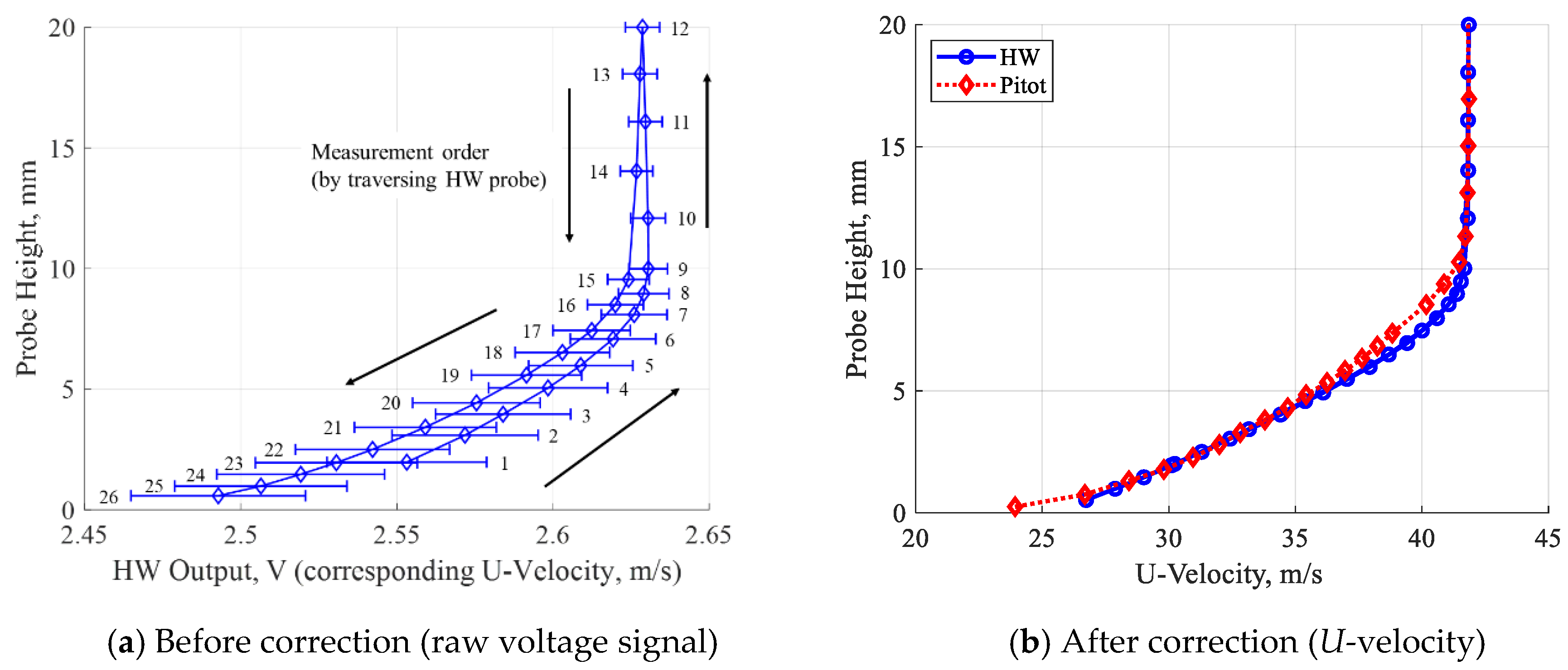
3.5. Quantitative Interpretation for Output Signals from Hot-Wire Anemometry

The output signal from hot-wire anemometry is a function of both the freestream velocity and freestream temperature. Therefore, it is necessary to convert the measured output signal to a quantitative velocity by applying an appropriate temperature correction method. If the temperature variation throughout the wind tunnel run is relatively small, the measured signal (i.e., voltage) can be regarded as a function of the flow velocity (i.e., Eoutput = f(U); f denotes a functional dependence), and King’s law [31], which is presented as Equation (25), can be applied:
E 2 = a + b U n   ; n = 0.45 ,
where constants a and b are determined by the calibration wind tunnel experiment to relate the voltage value and the freestream velocity.
However, if the temperature variation throughout the wind tunnel experiment is relatively large (as seen in Figure 5b), the temperature dependence can no longer be ignored and the measured signal must be regarded as a function of both the velocity and temperature (i.e., Eoutput = f(U, T)). In this case, a correction that considers temperature variations, such as the one expressed in Equation (26) [32], is useful:
U = v · f ( E 2 k Δ T ) = v · f ( E 2 k ( T w T a ) ) ,
where ν is the kinematic viscosity, and the coefficient k, which is the thermal conductivity of air, is determined by Equation (27) [33] using freestream temperature, Ta:
k = 418.4 ( 5.75 × 10 5 ( 1 + 3.17 × 10 3 T a 2.1 × 10 6 T a 2 ) ) .
Since the wire temperature, Tw, was unknown here and the flow temperature was measured at each probe height, Tw in Equation (26) was parametrically changed and its value that makes the difference of the U velocity profiles between the hot-wire anemometry data with Equation (26) and the pitot-rake data was sought to become zero or minimum. This modified temperature correction method with a best-fit approach was taken in this study for quantitative analysis. The resulting Tw values for each case are presented in Table 1 and this in-situ temperature correction was applied. Note that the derived Tw value includes not only the true wire temperature itself but also the correction effect of the output signal for a time decay as mentioned above. Those factors were considered to be the cause of the relatively large difference in Tw between smooth and riblet wall cases. It should also be noted that other temperature correction methods proposed in previous studies may be used, depending on the available dataset.
A representative profile of the raw output signal, which qualitatively corresponds to the U velocity, for the smooth wall is shown in Figure 9a. The measurement was carried out by fixing the probe position in the x- and y-directions, and traversed in the z-direction (height from the wall surface) as described in Figure 5a. The sequential numbers on the figure show the order of measurement, which are seen from Figure 5b. Each plotted point is a 15-s average, which corresponds to 300,000 data points. As stated above, the output signal strongly depends on the freestream temperature variation. Figure 9b plots the U velocity profiles after applying the temperature correction to the raw output signal of the hot-wire anemometry data. The profile obtained by the pitot-rake measurement is also plotted for comparison. The U velocity profile after temperature correction (HW) agrees with that determined by the pitot-rake measurement (Pitot). The maximum discrepancy between those two profiles around the boundary layer outer edge (9 mm) was 2.2%. It should be noted that the boundary layer thickness (δ), which was determined by the position where the local velocity value becomes 0.99U, was 10.2 mm (δsmooth = 10.2 mm) for this representative condition. The discrepancy excluding the region around the boundary layer outer edge was sufficiently small (i.e., 0.26% for z = 1.0–4.0 mm). Other hot-wire measurement data can be corrected similarly. Thus, the temperature correction with the best-fit approach can be considered as appropriate. The following discussion will be based on the temperature-corrected U velocity with respect to the hot-wire anemometry data by use of Equation (26).

4. Results and Discussion

This section discusses the insights gained from deriving turbulent integral scales and evaluating the reduction of skin friction drag by riblets and covers uncertainty analysis, characteristics of boundary layer profiles and turbulent scales, and reduction of skin friction drag by riblets.

4.1. Uncertainty Analysis

As mentioned in the introduction, reducing skin friction drag by applying riblets to a surface would be on the order of several percent. Therefore, it is vital to quantify the measurement uncertainty to demonstrate the effectiveness of applying the riblet surface to reduce skin friction drag. The possible sources of uncertainty in deriving the turbulent scale were found to be due to the wind tunnel freestream, measurement uncertainty by hot-wire anemometry, and the cumulative uncertainty in the postprocessing. Those sources and their values are listed in Table 2. Note that the uncertainty resulted in the temperature correction (q1) for the hot-wire anemometry data was considered at z = 1.0 mm as the measured U velocity at this height will be used to evaluate the skin friction drag reduction in a later section as mentioned before. The random uncertainty (q2) inherent in the hot-wire anemometry was represented by the temperature-corrected velocity variance in the freestream region (i.e., z = 12–20 mm: Five measurement points) for the smooth wall case for a duration of 5 s. The uncertainty that may be caused by the velocity fluctuations in the other components than the streamwise component was not obtained since the velocity measurement was conducted by a single-wire probe and therefore no exact three-dimensional velocity components were known.
Therefore, an assumption was made to estimate the uncertainty accounted for the other components of velocity fluctuations. Assuming that velocity variances exist in the streamwise direction (u’), spanwise direction (v’), and vertical direction (w’), the effective velocity (Ueff), which is the velocity information detected by the wire affected by u’, v’, and w’, can be expressed as follows. Here, the mean streamwise velocity that corresponds to the true velocity is U ¯ . The overbar indicates the time average. It should be noted that the flow direction to the wire sensor is assumed to be less than 30° [34] since the hot-wire probe was placed normal to the wall and the flow:
U e f f = ( U ¯ + u ʹ ) 2 + C H · v ʹ 2 + C K · w ʹ 2 ,
where CH and CK are directional sensitivity factors for each component of the flow [34]. By taking a time average and the Taylor series expansion, Equation (28) reduces to Equation (29):
U e f f U ¯ = 1 + 1 2 C H 2 v ʹ 2 ¯ U 2 ¯ + 1 2 C K 2 w ʹ 2 ¯ U 2 ¯ + O [ u ʹ 4 ¯ U 4 ¯ ] .
The last term in the right side in Equation (29) stands for the order of magnitude of remaining terms in the Taylor series expansion. Further rewriting Equation (29) by assuming that the velocity variances are small (i.e., | u ʹ / U ¯ | 1 ,   | v ʹ / U ¯ | 1 , and | w ʹ / U ¯ | 1 ), the uncertainty caused by the directional effect can be expressed as Equation (30):
U e f f U ¯ U ¯ 1 2 · T u · ( C H 2 + C K 2 ) ; T u =   1 3 ( u ʹ 2 ¯ + v ʹ 2 ¯ + w ʹ 2 ¯ ) U ¯ .
Tu is physically equivalent to the turbulent kinetic energy. Since exact values of v’ and w’ were unknown, it was roughly assumed that u’ = v’ = w’ for this analysis. Then, Tu can roughly be estimated as 0.1 near the wall (at z = 2 mm for the smooth wall; and the details will be presented in a later section). For the current probe geometry, CH and CK can be estimated as approximately 1.05 and 0.10, respectively [34]. Then, ( U e f f U ¯ ) / U ¯ 0.56 %   ( = q 3 ) . This error can be considered as a systematic error when implementing the hot-wire anemometry, and this error also contains the influence of the directional sensitivity.
The other systematic errors in the measurement can be neglected because the mean value of the fluctuating component of velocity was 0 and the histogram showed a nearly Gaussian distribution, which also will be presented in a later section. The uncertainty related to the freestream temperature variation and other uncertainties inherent in the freestream were included in the random uncertainty. Thus, the uncertainty generated by the hot-wire anemometry can be considered the governing source for the total uncertainty. The uncertainty in the velocity measurement by the hot-wire anemometry is given in Equation (31). Every error was considered to propagate independently:
q 123 [ % ] = q 1 2 + q 2 2 + q 3 2   = ( 0.26 100 ) 2 + 1 n i = 1 n ( U i U z = 12 20   m m ¯ U z = 12 20   m m ) 2 + ( 0.56 100 ) 2 × 100 = 0.62 % .
The uncertainty inherent in the calculation of the integral time scale was also considered. Since the autocorrelation function indicated a monotonically decreasing feature for the duration of interest, the uncertainty associated with the integration when calculating the integral time scale arises from the integration increment. The uncertainty in the integration with an increment of Δt = 5 μs was considered as following q4. Here, n is 5 for the measurement points in the freestream region:
q 4   [ % ] = 0.1 Δ t 1 n i = 1 n t 0 ,   i = 0.005 0.291 = 1.72 % .
Each uncertainty was considered to propagate independently, and thus the cumulative error of q1 through to q4 gives the total uncertainty (qtotal_1) for deriving the integral time scale. The total uncertainty for the derivation of the integral time scale can be estimated as 1.8% for n = 5 (measurement points in the freestream region) as shown below:
q t o t a l _ 1 = q 123 2 + q 4 2 = 1.83 % .
Note that the proposed method evaluates the reduction of skin friction drag based on the horizontal components of the turbulent scales and U velocity since the streamwise component of the velocity was focused on in this evaluation. It should also be noted that if the other components of the velocity fluctuations than the streamwise velocity fluctuation are obtained by other highly resolved measurements, such as three-dimensional measurements, the uncertainty may be reduced.

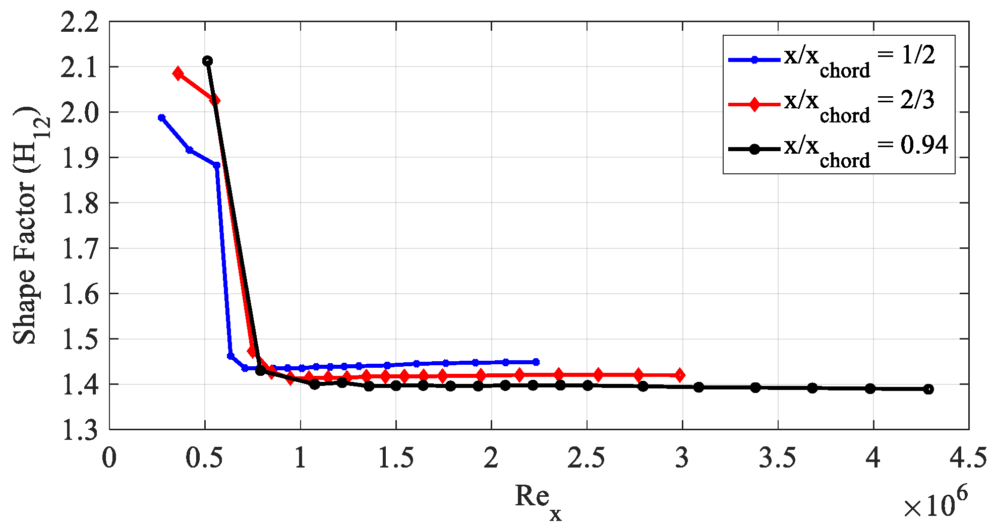
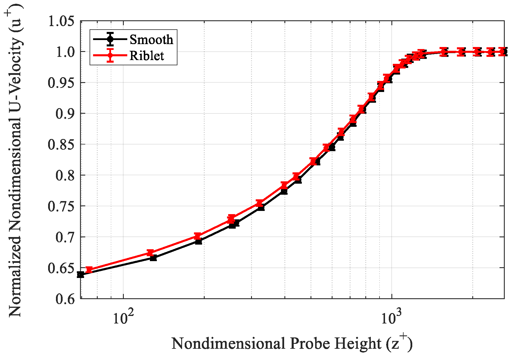
4.2. General Characteristics of Velocity Profiles

Figure 10 compares the U velocity profile of the smooth wall case with the riblet wall case obtained by hot-wire anemometry. The plotted data correspond to the temperature-corrected U velocity for an average duration of 15 s (N = 300,000 points) at each height point. The U velocity and the height were scaled to the nondimensional values u+ and z+, respectively, to emphasize the difference of the profile in the logarithmic region, where z+ appears to be in the order of 100. Nondimensional U velocity (u+) and height (z+) are expressed by Equation (34) and Equation (35), respectively. The friction velocity (uτ) expressed by Equation (5) was calculated using Equation (18) for the smooth wall case and Equation (23) for the riblet wall case, respectively. The reference height position for the smooth wall was z = 0 mm and that for the riblet wall was z = 50 μm as aforementioned. u+ was normalized by the maximum value for each wall surface to put an emphasis on comparing the U velocity in the logarithmic region:
u + = U u τ ,
z + = z · u τ v .
In Figure 10, the error bar range is the uncertainty q123 described previously. Above z+ = 500 (which corresponds to z = 4.5 mm), the difference between those two cases is negligibly small. On the other hand, in the region near the wall below z+ = 500, the riblet case shows a higher velocity than that of the smooth wall case. This observation is consistent with those obtained by previous studies [8,19].
Figure 11 presents histograms for the fluctuating component of the U velocity (u’) obtained by Reynolds decomposition (Equation (8)) at z = 2 mm (z/δsmooth = 0.196: Representing the boundary layer flowfield above the riblet peak) and at z = 20 mm (z/δsmooth = 19.6: Representing the freestream region) for the smooth wall. Because the boundary layer height was approximately 10 mm in this study and the effect of riblets on reducing skin friction drag should notably appear around the height of 20% to 30% of the boundary layer thickness from the wall [8], the study focused on the height of z = 2 mm. It should be noted here that the flow conditions were not identical to those of the former study [8]. The histogram for z = 20 mm shows a sharp distribution around its mean value and the variance is small. However, for z = 2 mm, the histogram shows a Gaussian distribution, indicating that the velocity variance can be treated as random data, which indicates isotropically homogeneous turbulence according to turbulence theory. Table 3 summarizes the statistical properties for the smooth wall and riblet cases with regard to the U velocity. The Kurtosis for z = 2 mm is approximately 3, which means that the distribution is Gaussian; the skewness for z = 2 mm also shows that the distribution is closer to being Gaussian. The turbulence intensity at z = 2 mm for the riblet surface shows an 8.3% reduction compared to the smooth surface. This observation is consistent with those found in previous studies [2,8,19].
In addition to those statistics, other boundary layer characteristics are summarized in Table 4. The boundary layer thickness for the smooth wall and riblet wall cases are δsmooth = 10.2 mm and δriblet = 10.2 mm, respectively. As seen in Table 4, the local boundary layer thicknesses (δ* and θ) and the local Reynolds number (Reθ) for the riblet case were reduced. If the reduction of total skin friction where the local skin friction coefficient (cf) in Equation (13) is replaced with the total skin friction coefficient (CF) expressed by Equation (22) is considered, the reduction of the total skin friction value becomes 3.1%. Therefore, the reduction of those boundary layer statistics is related to the reduction of skin friction drag. Note that Saravi et al. [2] concluded that the reduction of the turbulence intensity is indicative of the fact that the transition to turbulence in the viscous sub-layer was delayed [2]. The observation obtained in this study may be related to their results, but further study is needed to clarify it.

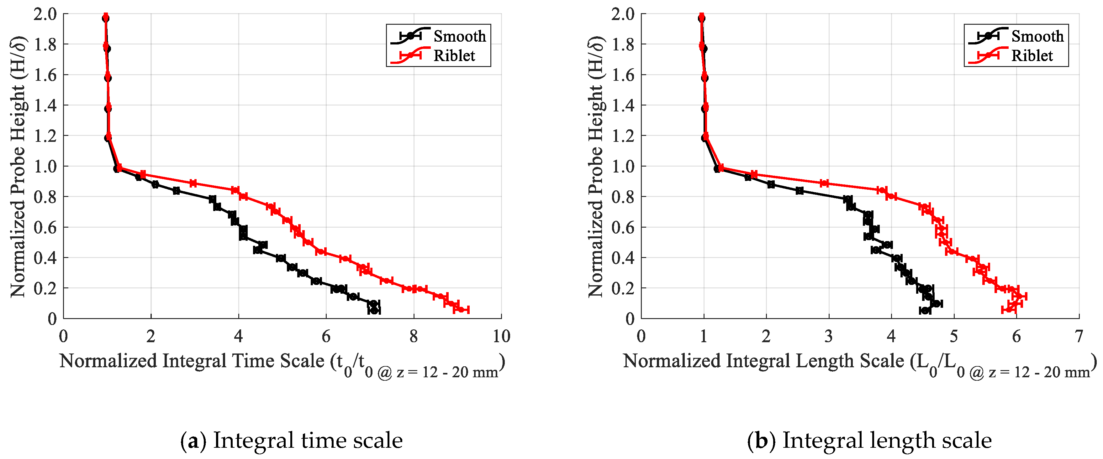
4.3. Integral Time and Length Scales

Figure 12a presents the integral time scale in the streamwise direction, which was computed by the method described in the previous section. The integral time scale was normalized by the mean value at the freestream (z = 12–20 mm). The error bar range is the uncertainty qtotal_1. The vertical axis representing the probe height was normalized by the boundary layer thickness: δsmooth = 10.2 mm for the smooth wall case and δriblet = 10.2 mm for the riblet wall case. It is obvious from Figure 12a that the integral time scale for the riblet surface is larger than that for the smooth wall in the entire boundary layer region and that the riblet case is 30% larger than that for the smooth wall case on average.
Figure 12b shows the derived integral length scale using Equation (12). The integral length scale was a product of the integral time scale and the mean U velocity. The uncertainty qtotal_1 is also shown as error bars. The same trend as in Figure 12a is seen in Figure 12b. Both the integral time and length scales for the riblet case are 30% larger compared to those for the smooth wall case. Since the integral time scale for the smooth wall case can be considered to be the life span of the turbulent structure and motion in the streamwise direction in the boundary layer, as a statistical average, the turbulent structure’s life span and scale in the streamwise direction for the riblet case near the wall were elongated. A similar observation was obtained by computer simulation with a similar configuration of three-dimensional sinusoidal riblets [15]. It is also notable that the integral length scale reaches the maximum at a height of 1 to 2 mm (or H/δ = 0.098–0.196) from the wall under the current flow conditions. It is emphasized that the previously reported insights gained by other techniques were observed by the proposed method in this study as well.

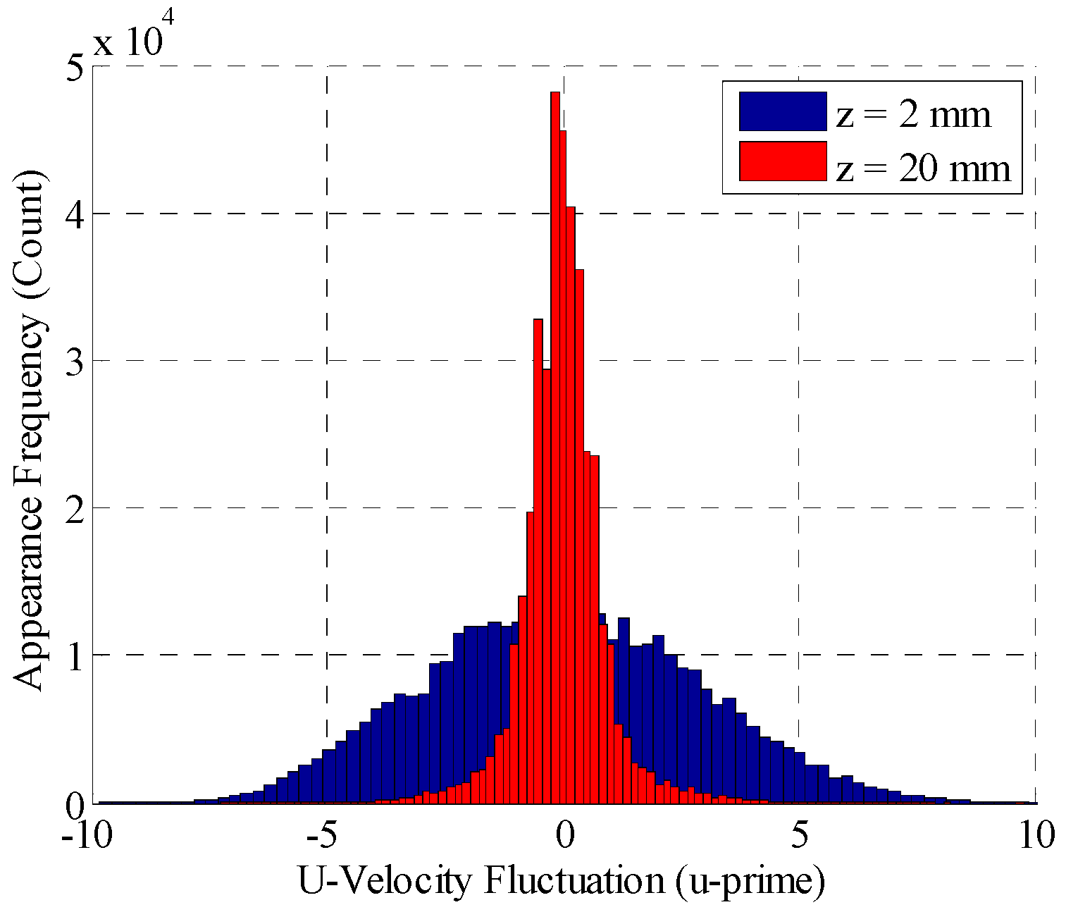
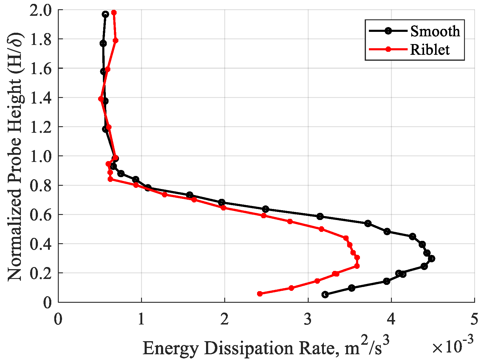
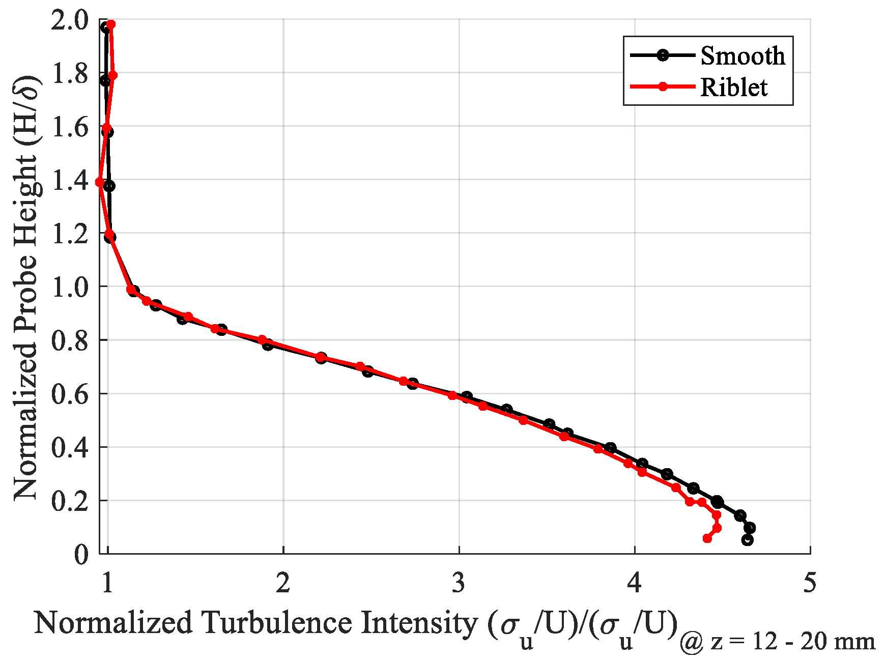
4.4. Smaller Scale Turbulence

Next, small-scale turbulence is discussed in this section. The small-scale turbulence is represented by the energy dissipation rate, which governs small-scale turbulence, which is more responsible for the energy dissipation. The energy dissipation rate is expressed as Equation (36) [35]. The energy dissipation rate is related more to the small-scale turbulent structure. In the energy cascade process, assuming that there is no energy loss, the energy produced by the large-scale turbulent motions is transferred to the small scales, which dissipate them:
ε = 0.697 σ u 3 L 0 .
Figure 13 compares the energy dissipation rates for the smooth wall case and the riblet wall. The probe height was also normalized by each boundary layer thickness for the smooth wall and riblet wall, respectively. Obviously, the riblet surface shows a much smaller distribution. Up to an 18% reduction is obtained using riblets. This physical interpretation indicates that the energy production was reduced in the riblet case. According to Viswanath [8], this can be attributed to the fact that the ejection motion was reduced by the riblets.
Figure 14 compares the profiles of the turbulence intensity for the smooth wall and the riblet wall. The turbulence intensity was calculated as σ u / U ¯ and normalized by the value in the freestream region. Though the turbulence intensity in the region above H/δ > 0.6 is identical between the smooth wall and riblet wall cases, the turbulence intensity near the wall for the riblet case appears to be smaller than that for the smooth wall case. This is consistent with the observation described in Table 3. Along with the observation obtained from Figure 13, the turbulence near the wall was reduced by the presence of the riblets.
This study showed that the large-scale turbulent structure in the streamwise direction became larger and the turbulence intensity became smaller by applying a riblet surface. A more detailed analysis, such as computer simulation or three-dimensional measurement with highly temporally and spatially resolved diagnostics, is needed to identify the key physics behind those observations and those responsible for the reduction of skin friction drag by applying the riblet surface, especially the present three-dimensional riblet surface.

4.5. Quantitative Evaluation of Reduction of Skin Friction Drag

The total uncertainty inherent in evaluating the skin friction drag reduction given by Equation (13) was considered to be the cumulative uncertainty of independently propagating sources of uncertainty. When solving Equation (13), the uncertainty (q5) is considered to be the difference of the calculated values in the freestream region from 0, because the skin friction drag in the freestream region should be 0. The total uncertainty is given by Equation (37), considering n measurement points and that each uncertainty propagates independently. For this calculation, n = 5, which corresponds to the number of measurement points in the freestream region (z = 12–20 mm):
q t o t a l [ % ] = ( q t o t a l _ 1 ) 2 + q 5 2 = ( 1.83 100 ) 2 + ( 0.68 100 ) 2 × 100 = 1.95 % .
Thus, the total uncertainty can be estimated at 2.0% for n = 5 (the number of measurement points in the freestream region) for evaluating the skin friction drag reduction. It should be noted that the uncertainty is governed by the uncertainty associated with the integration of the autocorrelation function as shown in Table 2, so the total uncertainty can be lowered further by reducing the uncertainty in integrating the autocorrelation function using smaller increments of Δt.
The reduction of the skin friction coefficient at z = 1.0 mm (above the riblet peak) was calculated at 2.8% using Equation (13), based on the hot-wire anemometry and the proposed method described in Section 3.4. Accounting for the total uncertainty of 2.0%, the effect of skin friction drag reduction by use of the paint-based riblet was demonstrated.
In order to support this evaluation, the skin friction drag reduction was compared to that obtained by the pitot-rake measurement [19] by applying the momentum integration method based on the U velocity profile in the boundary layer based on the pitot-rake measurement. First, the momentum thickness was calculated by Equation (2) based on the U velocity profile, then the total skin friction coefficient was calculated using Equation (22) [3], which can be applied to a two-dimensional flat plate surface with a zero-pressure gradient. The height ranged from 1.3 to 50.3 mm where the pitot-probe measurement was conducted. The control surface for calculating the total skin friction was from the virtual origin (x = 20 mm) where the disk roughness was placed at x = 600 mm where the pitot-probe measurement was done. The boundary layer was considered to be turbulent downstream from the virtual origin. By calculating the total skin friction coefficients from Equation (22) for the smooth wall and for the riblet wall, and by assuming that the local skin friction coefficient is proportional to the total skin friction coefficient, the skin friction drag reduction was obtained using Equation (13). Resultant skin friction drag reduction based on Equation (13) using the pitot-rake measurement was 2.9%. Although a slight difference between the pitot-tube-derived value and that obtained by the proposed method is seen (i.e., 0.1%), the derived value of the skin friction drag reduction by the proposed method is consistent with that by the pitot-rake data. Thus, the proposed method is appropriate.

5. Conclusions

A unique approach to evaluate the reduction of skin friction drag with an emphasis on the turbulent scales was applied to boundary layer profiles for a reference smooth wall surface and a riblet wall surface measured at the low-turbulence wind tunnel at the JAXA Chofu Aerospace Center. The riblets were fabricated from aircraft paint with a three-dimensional design. The riblet sheet was attached on the surface of a flat-plate test model. The boundary layer profile represented by the U velocity profile was measured by hot-wire anemometry and pitot-rake measurement. The measured raw output signal by the hot-wire anemometry was converted to the U velocity with appropriate temperature correction. Based on the measured boundary layer profiles, the following conclusions with regard to turbulence statistics and the validity of the proposed method evaluating the reduction of skin friction drag were drawn:
(1)
The riblet surface made from aircraft paint successfully demonstrated a reduction of skin friction drag.
(2)
The riblet surface increased both the integral time scale and the length scale by 30% from those for the smooth wall at a freestream velocity of 41.7 m/s (Mach 0.12) and a chord length of 67% (x/xchord = 2/3) from the model’s leading edge.
(3)
The proposed method evaluated the skin friction drag for the riblets at a freestream velocity of 41.7 m/s (Mach 0.12) and a chord length of 67% (x/xchord = 2/3) from the leading edge of the flat-plate model by 2.8%. This is consistent with that obtained by the momentum integration method based on the pitot-rake measurement of 2.9%.

Author Contributions

H.T. is responsible for the entire work from conceptualization, establishing methodology, data analysis, and writing the original manuscript entirely; M.K. managed the overall project and reviewed; H.I. and S.K. worked on wind tunnel experiments and raw data processing.

Funding

This research received no external funding.

Acknowledgments

This study was conducted as part of the Flight Investigation of Skin-Friction Reduction Eco-Coating (FINE) project by the JAXA Aeronautical Technology Directorate. The authors wish to thank the aerodynamics research unit and Tomonari Hirotani at the JAXA Aeronautical Technology Directorate for assistance with the wind tunnel experiment, and Akira Nishizawa for help with the hot-wire anemometry. The authors also wish to thank Kie Okabayashi for CFD simulation prior to the wind tunnel experiment. As for the riblet design, the authors acknowledge Masato Asai and Ayumi Inazawa at the Tokyo Metropolitan University, and Ryoko Shinohara at the Owell Incorporated. Also, the authors acknowledge Shihoko Endo and Kaoru Iwamoto at the Tokyo University of Agriculture and Technology for carrying out the experiment and for insightful help on research collaboration.

Conflicts of Interest

The authors declare no conflict of interest.

Nomenclature

A, B, Cconstant (coefficient)
CFtotal skin friction coefficient
CH, CKdirectional sensitivity factor
cflocal skin friction coefficient
ddiameter, mm
E voltage, V
fsampling frequency, Hz
H probe height, mm
H12 shape factor
h height of riblet, μm
k thermal conductivity, W/(m⋅K)
ks surface roughness, mm
L0integral length scale, mm
mdata length
Ndata length
quncertainty, %
R correlation coefficient
Re Reynolds number
s width of riblet, μm
s+ nondimensional width of riblet
T temperature, K or °C
Tu turbulent kinetic energy
t0integral time scale, s
Ustreamwise velocity component (U-velocity), m/s
u’ streamwise component of velocity fluctuation, m/s
u+ nondimensional U velocity
uτfriction velocity, m/s
v’ spanwise component of velocity fluctuation, m/s
w’ vertical component of velocity fluctuation, m/s
x coordinate in streamwise direction
y coordinate in spanwise direction
z coordinate in vertical direction
z+ nondimensional height
δ boundary layer thickness, mm
δ** displacement thickness, mm
ε energy dissipation rage, m2/s3
ν kinematic viscosity, m2/s
θ momentum thickness, mm
ρ density, kg/m3
σ standard deviation
τ0 Reynolds stress, Pa
Δt lag time, s

Subscripts

1, 2, 3…component number
Afreestream (air)
chord chord
effeffective
iindex number
laminarlaminar flow state
riblet riblet surface
smooth smooth surface
totaltotal
turbturbulent
uu velocity
wwire

References

  1. Szodruch, J. Viscous Drag Reduction on Transport Aircraft. In Proceedings of the 29th Aerospace Sciences Meeting, Reno, NV, USA, 7–10 January 1991. AIAA Paper 91-0685. [Google Scholar]
  2. Saravi, S.S.; Cheng, K. A Review of Drag Reduction by Riblets and Micro-Textures in the Turbulent Boundary Layers. Eur. Sci. J. 2013, 9, 62–81. [Google Scholar]
  3. Walsh, M.J. Viscous Drag Reduction in Boundary Layers; edited by Bushness and Hefner. Prog. Astronaut. Aeronaut. 1989, 123, 203–261. [Google Scholar]
  4. Walsh, M.J. Riblets as a Viscous Drag Reduction Technique. AIAA J. 1983, 21, 485–486. [Google Scholar] [CrossRef]
  5. Bushnell, D.M.; Hefner, J.N.; Ash, R.L. Effect of Compliant Wall Motion on Turbulent Boundary Layers. Phys. Fluids 1977, 20. [Google Scholar] [CrossRef]
  6. Suzuki, Y.; Kasagi, N. Turbulent Drag Reduction Mechanism Above a Riblet Surface. AIAA J. 1994, 32, 1781–1790. [Google Scholar] [CrossRef]
  7. Dean, B.; Bhushan, B. Shark-Skin Surfaces for Fluid-Drag Reduction in Turbulent Flow: A Review. Philos. Trans. R. Soc. A 2010, 368, 4775–4806. [Google Scholar] [CrossRef]
  8. Viswanath, P.R. Aircraft Viscous Drag Reduction Using Riblets. Prog. Aerosp. Sci. 2002, 38, 571–600. [Google Scholar] [CrossRef]
  9. Okabayashi, K. Direct Numerical Simulation for Modification of Sinusoidal Riblets. J. Fluid Sci. Technol. 2016, 11. [Google Scholar] [CrossRef]
  10. Sawyer, W.; Winter, K. An Investigation of the Effect on Turbulent Skin Friction of Surface with Streamwise Grooves. In Turbulent Drag Reduction by Passive Means, Proceedings of the International Conference, London, England, 15–17 September 1987; Royal Aeronautical Society: London, UK, 1987; pp. 330–362. [Google Scholar]
  11. Walsh, M.J. Turbulent Boundary Layer Drag Reduction Using Riblets. In Proceedings of the 20th Aerospace Sciences Meeting, Orlando, FL, USA, 11–14 January 1982. AIAA Paper 82-0169. [Google Scholar]
  12. Bechert, D.W.; Bruse, M.; Hage, W.; Van Der Hoeven, J.G.T.; Hoppe, G. Experiments on Drag-Reducing Surfaces and their Optimization with an Adjustable Geometry. J. Fluid Mech. 1997, 338, 59–87. [Google Scholar] [CrossRef]
  13. MBB Transport Aircraft Group. Microscopic Rib Profiles Will Increase Aircraft Economy in Flight. Aircr. Eng. 1988, 60, 11. [Google Scholar] [CrossRef]
  14. Grüneberger, R.; Kramer, F.; Wassen, E.; Hage, W.; Meyer, R.; Thiele, F. Influence of Wave-Like Riblets on Turbulent Friction Drag. Nat. Inspired Fluid Mech. 2012, 119, 311–329. [Google Scholar]
  15. Peet, Y.; Sagaut, P.; Charron, Y. Turbulent Drag Reduction using Sinusoidal Riblets with Triangular Cross-Section. In Proceedings of the 38th Fluid Dynamics Conference and Exhibit, Seattle, WA, USA, 23–26 June 2008. AIAA Paper 2008-3745. [Google Scholar]
  16. Peet, Y.; Sagaut, P.; Charron, Y. Pressure Loss Reduction in Hydrogen Pipelines by Surface Restructuring. Int. J. Hydrogen Energy 2009, 34, 8964–8973. [Google Scholar] [CrossRef]
  17. Peet, Y.; Sagaut, P. Theoretical Prediction of Turbulent Skin Friction on Geometrically Complex Surfaces. Phys. Fluids 2009, 21, 10. [Google Scholar] [CrossRef]
  18. Kurita, M.; Nishizawa, A.; Okabayashi, K.; Koga, S.; Kwak, T.; Nakakita, K.; Naka, Y. FINE: Flight Investigation of Skin-Friction Reducing Eco-Coating. In Proceedings of the 54th Aircraft Symposium, Toyama, Japan, 24–26 October 2016. JSASS-2016-5180 (In Japanese). [Google Scholar]
  19. Koga, S.; Kurita, M.; Iijima, H.; Okabayashi, K.; Nishizawa, A.; Takahashi, H.; Endo, S. Wind Tunnel Tests for Measurement System Design of Flight Investigation of Skin-Friction Reducing Eco-Coating (FINE). In Proceedings of the 54th Aircraft Symposium, Toyama, Japan, 24–26 October 2016. JSASS-2016-5105 (In Japanese). [Google Scholar]
  20. Liu, T. Extraction of Skin-Friction Fields from Surface Flow Visualizations as an Inverse Problem. Meas. Sci. Technol. 2013, 24, 124004. [Google Scholar] [CrossRef]
  21. Bottini, H.; Kurita, M.; Iijima, H.; Fukagata, K. Effects of Wall Temperature on Skin-Friction Measurements by Oil-Film Interferometry. Meas. Sci. Technol. 2015, 26, 105301. [Google Scholar] [CrossRef]
  22. Takahashi, H.; Tomioka, S.; Sakuranaka, N.; Tomita, T.; Kuwamori, K.; Masuya, G. Effects of Plume Impingements of Clustered Nozzles on the Surface Skin Friction. J. Propuls. Power 2015, 31, 485–495. [Google Scholar] [CrossRef]
  23. Marshakov, A.V.; Scheta, J.A.; Kiss, T. Direct Measurement of Skin Friction in a Turbine Cascade. J. Propuls. Power 1996, 12, 245–249. [Google Scholar] [CrossRef]
  24. Takahashi, H.; Kurita, M.; Koga, S.; Endo, S. Turbulent Boundary Layer Characteristics of Riblet Surface Responsible for Skin Friction Drag. In Proceedings of the 54th Aircraft Symposium, Toyama, Japan, 24–26 October 2016. JSASS-2016-5102 (In Japanese). [Google Scholar]
  25. Schlichting, H.; Gersten, K. Boundary Layer Theory: 8th Revised and Enlarged Edition; Springer: Berlin, Germany, 1999; p. 436. [Google Scholar]
  26. Stenzel, V.; Wilke, Y.; Hage, W. Drag-Reducing Paints for the Reduction of Fuel Consumption in Aviation and Shipping. Prog. Org. Coat. 2011, 70, 224–229. [Google Scholar] [CrossRef]
  27. Potter, M.C.; Wiggert, D.C.; Ramadan, B.; Shin, T.I.-P. Mechanics of Fluids; Cengage Learning: Boston, MA, USA, 2015; p. 393. [Google Scholar]
  28. Takahashi, H.; Kanamori, M.; Naka, Y.; Makino, Y. Statistical Characterization of Atmospheric Turbulence Behavior Responsible for Sonic Boom Waveform Deformation. AIAA J. 2018, 56, 673–686. [Google Scholar] [CrossRef]
  29. Chanson, H. Applied Hydrodynamics: An. Introduction; CRC Press: Boca Raton, FL, USA, 2014; p. 293. [Google Scholar]
  30. Houghton, E.L.; Carpenter, P.W.; Colicott, S.H.; Valentine, D.T. Aerodynamics for Engineering Students 6th Edition; Elsevier: Amsterdam, The Netherlands, 2013; p. 557. [Google Scholar]
  31. King, L.B. On the Convection of Heat From Small Cylinders in a Stream of Fluid: Determination of the Convection Constants of Small Platinum Wires, with Applications to Hot-Wire Anemometry. Proc. R. Soc. A 1914, 90. [Google Scholar] [CrossRef]
  32. Hultmark, M.; Smits, A.J. Temperature Corrections for Constant Temperature and Constant Current Hot-Wire Anemometers. Meas. Sci. Technol. 2010, 21, 105404. [Google Scholar] [CrossRef]
  33. Kannuluik, W.G.; Carman, E.H. The Temperature Dependence of the Thermal Conductivity of Air. Aust. J. Sci. Res. Ser. A Phys. Sci. 1951, 4, 305–314. [Google Scholar] [CrossRef]
  34. Lomas, C.G. Fundamentals of Hot Wire Anemometry; Cambridge University Press: Cambridge, UK, 1986; Chapter 2. [Google Scholar]
  35. Frehlich, R.; Meillier, Y.; Jensen, M.L.; Balsley, B. Measurements of Boundary Layer Profiles in an Urban Environment. J. Appl. Meteorol. Climatol. 2006, 45, 821–837. [Google Scholar] [CrossRef]
Figure 1. Schematic illustration of the flat-plate test model installed at the center of the wind tunnel duct.
Applsci 09 05199 g001
Figure 2. Geometry of the leading edge of the flat-plate model.
Applsci 09 05199 g002
Figure 3. Shape factor (H12) for different freestream conditions and measurement locations.
Applsci 09 05199 g003
Figure 4. Details of riblet geometry: top view (upper figure) and side view (lower figure).
Applsci 09 05199 g004
Figure 5. Schematic diagram of hot-wire anemometry (a) and freestream temperature change for a representative smooth wall case during wind tunnel operation (b).
Applsci 09 05199 g005
Figure 6. Illustration of pitot-rake assembly attached to the flat plate model surface.
Applsci 09 05199 g006
Figure 7. Illustration of the computation of the integral time scale.
Applsci 09 05199 g007
Figure 8. Procedure for deriving unknown coefficients A and B for evaluating the skin friction coefficient.
Applsci 09 05199 g008
Figure 9. U-velocity profiles for the smooth wall case.
Applsci 09 05199 g009
Figure 10. Comparison of U-velocity profiles for smooth wall and riblet cases.
Applsci 09 05199 g010
Figure 11. Histograms of the fluctuating component of the U-velocity for a smooth wall.
Applsci 09 05199 g011
Figure 12. Normalized integral time and length scales normalized by the value in the freestream region.
Applsci 09 05199 g012
Figure 13. Profiles of energy dissipation rate.
Applsci 09 05199 g013
Figure 14. Profiles of turbulence intensities.
Applsci 09 05199 g014
Table 1. Summary of temperature correction.
Wall TypeMean Freestream VelocityTw, °C
Smooth41.7 m/s (Mach 0.12)111
Riblet41.7 m/s (Mach 0.12)77
Table 2. Summary of possible uncertainty sources.
Uncertainty SourceSymbolValue, %Note
Temperature correctionq10.26Obtained from the difference between the temperature corrected hot-wire data and the pitot probe data for z = 1.0–4.0 mm
Hot-wire anemometryq20.035 + 0.05Variance from five measurement points in the freestream region (z = 12–20 mm)
Systematic errorq30.56Equations. (28) through (30) accounting for the directional sensitivity of the velocity measurement
Derivation of integral time scaleq41.72q4 = 0.1Δt/(t0: freestream in smooth wall) = 0.005 ms/0.291 ms
Table 3. Statistical properties for smooth wall and riblet surfaces.
Statistical PropertiesSmooth WallRiblet
z = 2 mm
(z/δsmooth = 0.196: Inside the Boundary Layer)
z = 20 mm
(z/δsmooth = 19.6: Freestream Region)
z = 2 mm
(z/δsmooth = 0.198: Inside the Boundary Layer)
z = 20 mm
(z/δsmooth = 19.8: Freestream Region)
Mean ( U ¯ ), m/s30.1041.8530.4141.83
Standard deviation (σu), m/s2.880.892.680.85
Kurtosis, m/s2.768.362.769.13
Skewness, m/s0.130.280.150.26
Turbulence intensity ( σ u / U ¯ )0.0960.0210.0880.020
Table 4. Boundary layer characteristics covering boundary layer thicknesses and Reynolds numbers.
Wall Typeδδ*θReδReθ
Smooth Wall10.21.631.242.66 × 1043.22 × 104
Riblet10.21.561.202.66 × 1043.12 × 104

