Enhanced Evolutionary Sizing Algorithms for Optimal Sizing of a Stand-Alone PV-WT-Battery Hybrid System

 , , , , and
Abstract
1. Introduction
- A model based on HRESs is proposed, where a PV-WT-battery system and its components are formulated and elaborated.
- Meta-heuristic algorithms: teaching-learning based optimization (TLBO), enhanced differential evolution (EDE), and salp swarm algorithm (SSA) are firstly used to find the optimal number of HRESs with an objective function to minimize the user’s TAC in an SA environment.
- Two novel hybrid approaches based on combining (TLBO + EDE and TLBO + SSA) are also proposed for the better exploitation of the search space. These hybrid approaches are called enhanced evolutionary sizing algorithms (EESAs).
- The results obtained by EESAs are compared to their ancestor schemes in three different scenarios: PV-WT-battery, PV-battery, and WT-battery systems for a yearly user’s load profile. Further, the real solar irradiation and wind speed data are used, which are obtained from Rafsanjan, Iran.
- The reliability of HRESs is considered using four maximum allowable LPSP () values: 0%, 0.5%, 1%, and 3%, which are provided by the user. The TACs at different values are presented and analyzed.
2. System Model
3. Formulation of HRESs
3.1. Formulation of the PV System
3.2. Formulation of the WT System
3.3. Formulation of User’s Load
3.4. Excess and Deficit Cases of HRESs and Sizing of the Batteries
3.5. Formulation of the System’s Reliability
3.6. Total Annual Cost Modeling and Constraints
3.6.1. Objective Function Formulation
3.6.2. Constraints
4. Proposed Algorithms for the Unit Sizing Problem
4.1. TLBO
4.2. EDE
4.3. SSA
4.4. EESAs
- (i)
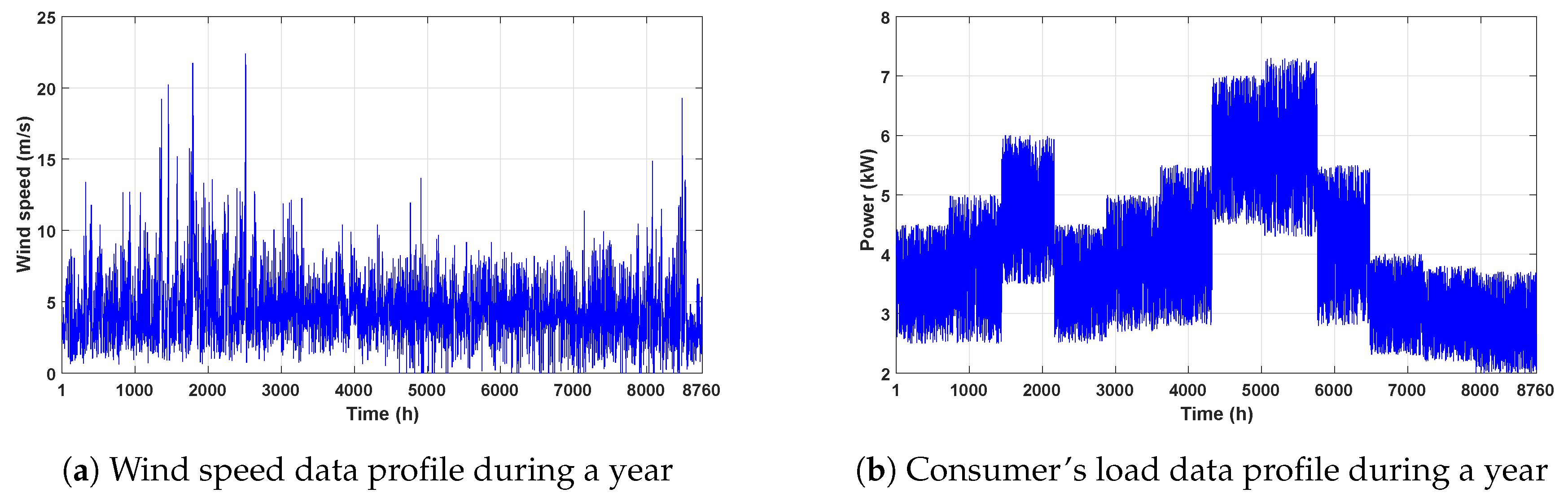
- The first step includes initialization of parameters: hourly input solar irradiation, ambient temperature, the speed of the wind, and user’s load profile data.
- (ii)
- (iii)
- In the third step, a solution space of two decision variables is randomly generated within the upper and lower bounds as given below.In Equation (34), the first and second columns are associated with the number of PVs and WTs, respectively.
- (iv)
- In this step, based on the RESs’ generation and user’s load, the total number of batteries required for each j solution is calculated using Equation (8). Thus, the cluster of configurations showing the solution space is depicted as:Here, the third column shows the total number of batteries in the battery bank. In Equation (35), for the population generation, represents j possible configurations. Each configuration represents a possible solution competing to fulfill the EESA objective.
- (v)
- (vi)
- Here, each configuration is evaluated using fitness criteria as depicted in Equation (10).The fitness value of each configuration shows the respective TAC, which is obtained by the summation of capital and maintenance costs.
- (vii)
- Here, TLBO steps are applied to update the population. First, the mean M of the learners is calculated subject wise. The best learner based on is chosen as a teacher. The mean of learners is shifted toward the teacher via Equation (23). In the learner phase, the population is updated using Equation (25). The new solution is accepted only if it gives a better TAC value. The new population is called .
- (viii)
- (ix)
- Steps (iv)–(viii) are repeated by the EESA process until the global termination criterion of 100 generations is satisfied.
- (x)
- Lastly, the global best solution among 100 generations based on the TAC value is returned. The global best solution contains the respective number of , , , TAC, and LPSP values.
5. Results and Discussion
- (i)
- PV-WT-battery: (),
- (ii)
- PV-battery: (), and
- (iii)
- WT-battery: ().
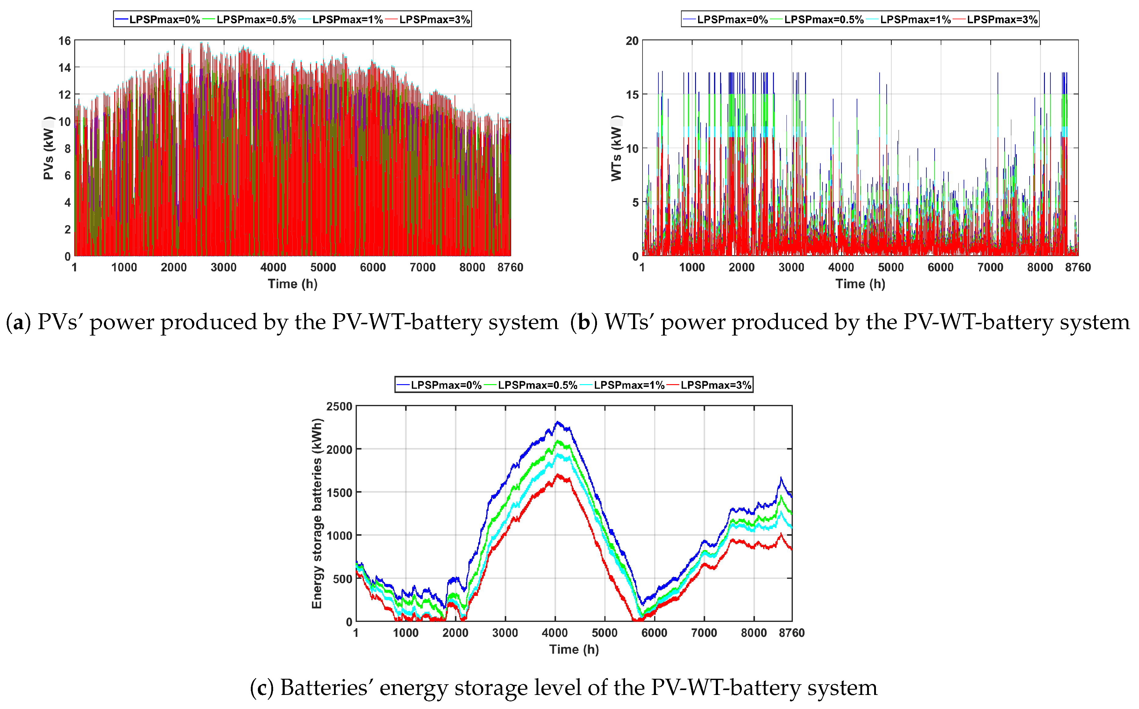
5.1. Scenario 1: PV-WT-Battery Hybrid System ()
- at ,
- at ,
- at , and
- at .
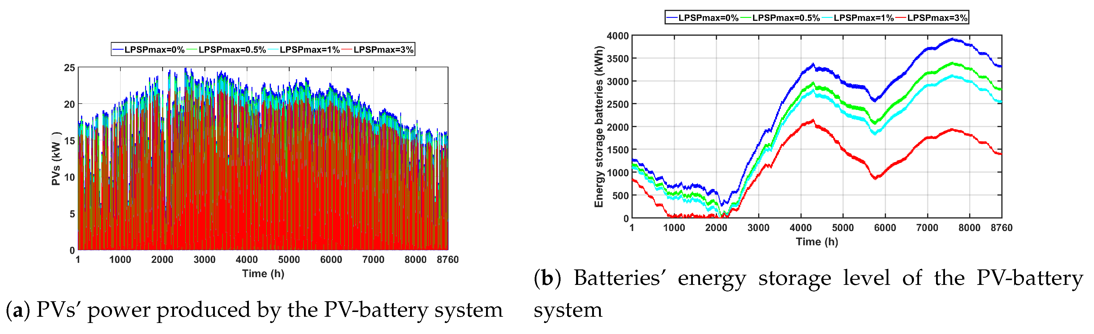
5.2. Scenario 2: PV-Battery System ()
- at ,
- at ,
- at , and
- at .
5.3. Scenario 3: WT-Battery System ()
- at ,
- at ,
- at , and
- at .
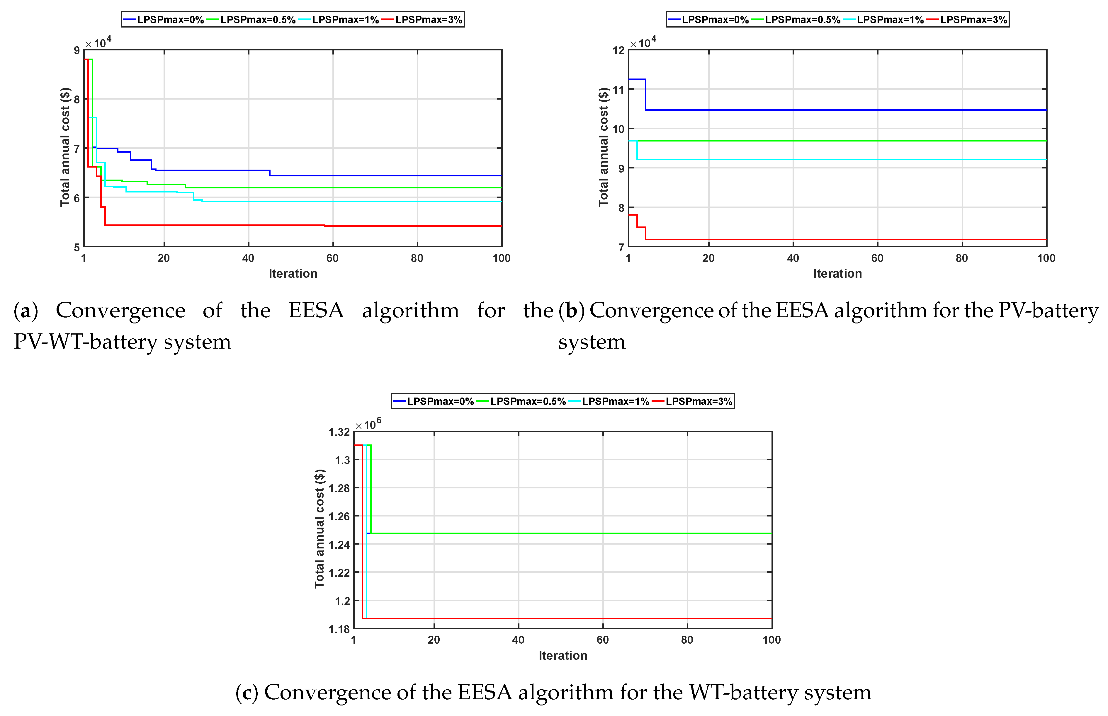
5.4. Convergence Process of the EESA Algorithm for Three Scenarios
6. Conclusions and Future Work
- (i)
- Hybrid EESAs were developed for better exploration and exploitation of the search space. EESAs accepted inputs, including solar irradiation, ambient temperature, wind speed, and user’s load data.
- (ii)
- The PV-WT-battery hybrid system was found with the best optimal configuration of RESs with reduced TACs as compared to the PV-battery and WT-battery systems. The TACs achieved by EESA were $64,430, $61,970, $59,200, and $54,171 at values of 0%, 0.5%, 1%, and 3%, respectively. In the PV-WT-battery hybrid system, the algorithms EESA, TLBO, EDE, and SSA were ranked as 1st, 2nd, 3rd, and 4th, respectively, based on their average TAC values. EESA performed better than other algorithms due to the better search on more promising areas of the solution space. On the other hand, TLBO’s performance was found better compared to the EDE and SSA schemes because it neither required any algorithm specific parameter, nor its calibration to obtain the optimal results.
- (iii)
- The PV-battery system provided the second most economical results. The TACs achieved were $104,640, $96,840, $92,120, and $71,790 at values of 0%, 0.5%, 1%, and 3%, respectively. In this scenario, EESA and TLBO performed equally and were placed in the first category. EDE and SSA achieved second and third rankings based on their average TACs, respectively.
- (iv)
- The third scenario: The WT-battery system was the most expensive case, due to the high price of WTs. The TACs $124,750 and $118,690 were achieved by EESA at values of (0%, 0.5%) and (1%, 3%), respectively. Here, all algorithms achieved the same optimal results due to a fewer number of decision variables compared to the PV-WT-battery hybrid system, thus being ranked equally.
- (v)
- The trade-off analysis between TAC and was also evaluated. It was found that when the values were increased from 0%, TACs were minimized and vice versa.
Author Contributions
Funding
Conflicts of Interest
Abbreviations
| CRF | Capital recovery factor | ||
| DE | Differential evolution | ||
| DoD | Depth of discharge | ||
| EESAs | Enhanced evolutionary sizing algorithms | ||
| EDE | Enhanced differential evolution | ||
| ESSs | Energy storage systems | ||
| FF | Fossil fuel | ||
| GA | Genetic algorithm | ||
| HOMER | Hybrid optimization model for electric renewables | ||
| HRESs | Hybrid renewable energy sources | ||
| HT | Hybrid technique | ||
| LPSP | Loss of power supply probability | ||
| NSGA-II | Non-dominated sorting genetic algorithm II | ||
| PSO | Particle swarm optimization | ||
| PV | Photovoltaic | ||
| RESs | Renewable energy sources | ||
| SA | Stand-alone | ||
| SSA | Salp swarm algorithm | ||
| SoC | State of charge | ||
| TAC | Total annual cost | ||
| TLBO | Teaching-learning based optimization | ||
| TS | Tabu search | ||
| WT | Wind turbine | ||
| Acronyms | |||
| Total cost | Capital cost | ||
| Maintenance cost | Present battery worth | ||
| Present worth of the inverter/converter | Unit cost of WT | ||
| Unit cost of the PV panel | Unit cost of the battery unit | ||
| Unit cost of the inverter/converter | Annual maintenance costs of PV panels | ||
| Annual maintenance costs of WTs | Total PV generated power | ||
| Overall produced wind power | User’s load | ||
| Energy stored at time slots t | |||
| Energy stored at time slots | Salp new population | ||
| i | Appliance | ||
| Self-discharging state | Interest rate | ||
| Solar radiation | Solar radiation at reference conditions | ||
| Loss of power supply probability | Maximum allowable LPSP value | ||
| Maximum generation point | Minimum generation point | ||
| Mean of the learners | Mutant vector | ||
| Efficiency of the inverter | Battery bank charging efficiency | ||
| n | System’s life span in years | Total number of batteries in the battery bank | |
| Number of WTs | Maximum number of PV panels | ||
| Maximum number of batteries | Maximum number of WTs | ||
| Present price of the inverter/converter | Present battery price | ||
| Power rating | Total hourly PV panel power output | ||
| Rated PV power | Output power generated by the WT | ||
| Nominal rated WT power | or r | Random number | |
| Target vector | s | Number of decision variables | |
| S | Row vector of positive integers | or | New vector |
| or | Old vector | Teacher in the TLBO process | |
| or | Learner 1 | or | Learner 2 |
| t | Time slot | Temperature coefficient of PV panels | |
| Cell temperature | Ambient air temperature | ||
| Normal operating cell temperature | Teaching factor | ||
| or | Trial vector | v | Wind speed |
| Rated wind speed | Cut-out wind speed | ||
| Cut-in wind speed | Boolean integer | ||
References
- Wang, X.; Palazoglu, A.; El-Farra, N.H. Operational optimization and demand response of hybrid renewable energy systems. Appl. Energy 2015, 143, 324–335. [Google Scholar] [CrossRef]
- California Energy Commission. 2008. Available online: https://www.energy.ca.gov/renewables/ (accessed on 24 November 2018).
- Yilmaz, S.; Dincer, F. Optimal design of hybrid PV-Diesel-Battery systems for isolated lands: A case study for Kilis, Turkey. Renew. Sustain. Energy Rev. 2017, 77, 344–352. [Google Scholar] [CrossRef]
- Ayodele, T.R.; Ogunjuyigbe, A.S.O. Wind energy potential of Vesleskarvet and the feasibility of meeting the South African’s SANAE IV energy demand. Renew. Sustain. Energy Rev. 2016, 56, 226–234. [Google Scholar] [CrossRef]
- Ogunjuyigbe, A.S.O.; Ayodele, T.R.; Akinola, O.A. Optimal allocation and sizing of PV/Wind/Split-diesel/Battery hybrid energy system for minimizing life cycle cost, carbon emission and dump energy of remote residential building. Appl. Energy 2016, 171, 153–171. [Google Scholar] [CrossRef]
- Ayodele, T.R.; Ogunjuyigbe, A.S.O. Mitigation of wind power intermittency: Storage technology approach. Renew. Sustain. Energy Rev. 2015, 44, 447–456. [Google Scholar] [CrossRef]
- Ranaboldo, M.; Ferrer-Marti, L.; Garcia-Villoria, A.; Moreno, R.P. Heuristic indicators for the design of community off-grid electrification systems based on multiple renewable energies. Energy 2013, 50, 501–512. [Google Scholar] [CrossRef]
- Zhang, W.; Maleki, A.; Rosen, M.A.; Liu, J. Sizing a stand-alone solar-wind-hydrogen energy system using weather forecasting and a hybrid search optimization algorithm. Energy Convers. Manag. 2019, 180, 609–621. [Google Scholar] [CrossRef]
- Yang, H.; Zhou, W.; Lu, L.; Fang, Z. Optimal sizing method for stand-alone hybrid solar-wind system with LPSP technology by using genetic algorithm. Sol. Energy 2008, 82, 354–367. [Google Scholar] [CrossRef]
- Yang, H.; Lu, L.; Zhou, W. A novel optimization sizing model for hybrid solar-wind power generation system. Sol. Energy 2007, 81, 76–84. [Google Scholar] [CrossRef]
- Aziz, N.I.A.; Sulaiman, S.I.; Shaari, S.; Musirin, I.; Sopian, K. Optimal sizing of stand-alone photovoltaic system by minimizing the loss of power supply probability. Sol. Energy 2017, 150, 220–228. [Google Scholar] [CrossRef]
- Abbas, F.; Habib, S.; Feng, D.; Yan, Z. Optimizing Generation Capacities Incorporating Renewable Energy with Storage Systems Using Genetic Algorithms. Electronics 2018, 7, 100. [Google Scholar] [CrossRef]
- Baghdadi, F.; Mohammedi, K.; Diaf, S.; Behar, O. Feasibility study and energy conversion analysis of stand-alone hybrid renewable energy system. Energy Convers. Manag. 2015, 105, 471–479. [Google Scholar] [CrossRef]
- Bhandari, B.; Lee, K.T.; Lee, C.S.; Song, C.K.; Maskey, R.K.; Ahn, S.H. A novel off-grid hybrid power system comprised of solar photovoltaic, wind, and hydro energy sources. Appl. Energy 2014, 133, 236–242. [Google Scholar] [CrossRef]
- Hurtado, E.; Peralvo-Lopez, E.; Perez-Navarro, A.; Vargas, C.; Alfonso, D. Optimization of a hybrid renewable system for high feasibility application in non-connected zones. Appl. Energy 2015, 155, 308–314. [Google Scholar] [CrossRef]
- Khan, A.; Javaid, N.; Khan, M.I. Time and device based priority induced comfort management in smart home within the consumer budget limitation. Sustain. Cities Soc. 2018, 41, 538–555. [Google Scholar] [CrossRef]
- Ahmad, A.; Khan, A.; Javaid, N.; Hussain, H.M.; Abdul, W.; Almogren, A.; Alamri, A.; Azim Niaz, I. An optimized home energy management system with integrated renewable energy and storage resources. Energies 2017, 10, 549. [Google Scholar] [CrossRef]
- Khan, A.; Javaid, N.; Ahmad, A.; Akbar, M.; Khan, Z.A.; Ilahi, M. A priority-induced demand side management system to mitigate rebound peaks using multiple knapsack. J. Ambient Intell. Humaniz. Comput. 2019, 10, 1655–1678. [Google Scholar] [CrossRef]
- Hussain, B.; Javaid, N.; Hasan, Q.; Javaid, S.; Khan, A.; Malik, S. An Inventive Method for Eco-Efficient Operation of Home Energy Management Systems. Energies 2018, 11, 3091. [Google Scholar] [CrossRef]
- Khan, A.; Javaid, N.; Javaid, S. Optimum unit sizing of stand-alone PV-WT-Battery hybrid system components using Jaya. In Proceedings of the 2018 IEEE 21st International Multi-Topic Conference (INMIC), Karachi, Pakistan, 1–2 November 2018; pp. 1–8. [Google Scholar]
- Khan, A.; Javaid, N.; Rafique, A. Optimum unit sizing of a stand-alone hybrid PV-WT-FC system using Jaya algorithm. In Proceedings of the International Conference on Cyber Security and Computer Science (ICONCS), Karabuk University (KBU), Karabuk, Turkey, 18–20 October 2018. [Google Scholar]
- Ghorbani, N.; Kasaeian, A.; Toopshekan, A.; Bahrami, L.; Maghami, A. Optimizing a hybrid wind-PV-battery system using GA-PSO and MOPSO for reducing cost and increasing reliability. Energy 2018, 154, 581–591. [Google Scholar] [CrossRef]
- Belouda, M.; Hajjaji, M.; Sliti, H.; Mami, A. Bi-objective optimization of a standalone hybrid PV-Wind-battery system generation in a remote area in Tunisia. Sustain. Energy Grids Netw. 2018, 16, 315–326. [Google Scholar] [CrossRef]
- Wang, R.; Li, G.; Ming, M.; Wu, G.; Wang, L. An efficient multi-objective model and algorithm for sizing a stand-alone hybrid renewable energy system. Energy 2017, 141, 2288–2299. [Google Scholar] [CrossRef]
- Hazem Mohammed, O.; Amirat, Y.; Benbouzid, M. Economical Evaluation and Optimal Energy Management of a Stand-Alone Hybrid Energy System Handling in Genetic Algorithm Strategies. Electronics 2018, 7, 233. [Google Scholar] [CrossRef]
- Goel, S.; Sharma, R. Optimal sizing of a biomass-biogas hybrid system for sustainable power supply to a commercial agricultural farm in northern Odisha, India. Environ. Dev. Sustain. 2019, 21, 2297–2319. [Google Scholar] [CrossRef]
- He, L.; Zhang, S.; Chen, Y.; Ren, L.; Li, J. Techno-economic potential of a renewable energy-based microgrid system for a sustainable large-scale residential community in Beijing, China. Renew. Sustain. Energy Rev. 2018, 93, 631–641. [Google Scholar] [CrossRef]
- Luta, D.N.; Raji, A.K. Optimal sizing of hybrid fuel cell-supercapacitor storage system for off-grid renewable applications. Energy 2019, 166, 530–540. [Google Scholar] [CrossRef]
- Maleki, A.; Pourfayaz, F. Optimal sizing of autonomous hybrid photovoltaic/wind/battery power system with LPSP technology by using evolutionary algorithms. Sol. Energy 2015, 115, 471–483. [Google Scholar] [CrossRef]
- Khan, A.; Javaid, N.; Khan, S.; Saba, T.; Khan, W.; Sattar, N.A. Enhanced Differential Evolutionary Algorithm for Optimal Sizing of Stand-alone PV-WT-Battery System considering Loss of Power Supply Probability Concept. In Proceedings of the 10th IEEE GCC Conference and Exhibition, Kuwait, 19–23 April 2019. [Google Scholar]
- Mohammadi, M.; Hosseinian, S.H.; Gharehpetian, G.B. Optimization of hybrid solar energy sources/wind turbine systems integrated to utility grids as microgrid (MG) under pool/bilateral/hybrid electricity market using PSO. Sol. Energy 2012, 86, 112–125. [Google Scholar] [CrossRef]
- Kellogg, W.D.; Nehrir, M.H.; Venkataramanan, G.; Gerez, V. Generation unit sizing and cost analysis for stand-alone wind, photovoltaic, and hybrid wind/PV systems. IEEE Trans. Energy Convers. 1998, 13, 70–75. [Google Scholar] [CrossRef]
- Rao, R.V.; Savsani, V.J.; Vakharia, D.P. Teaching-learning-based optimization: A novel method for constrained mechanical design optimization problems. Comput.-Aided Des. 2011, 43, 303–315. [Google Scholar] [CrossRef]
- Arafa, M.; Sallam, E.A.; Fahmy, M.M. An enhanced differential evolution optimization algorithm. In Proceedings of the 2014 Fourth International Conference on Digital Information and Communication Technology and its Applications (DICTAP), Bangkok, Thailand, 6–8 May 2014; pp. 216–225. [Google Scholar]
- Mirjalili, S.; Gandomi, A.H.; Mirjalili, S.Z.; Saremi, S.; Faris, H.; Mirjalili, S.M. Salp Swarm Algorithm: A bio-inspired optimizer for engineering design problems. Adv. Eng. Softw. 2017, 114, 163–191. [Google Scholar] [CrossRef]
- Sinha, S.; Chandel, S.S. Review of recent trends in optimization techniques for solar photovoltaic-wind based hybrid energy systems. Renew. Sustain. Energy Rev. 2015, 50, 755–769. [Google Scholar] [CrossRef]
- Javaid, N.; Ahmed, A.; Iqbal, S.; Ashraf, M. Day ahead real time pricing and critical peak pricing based power scheduling for smart homes with different duty cycles. Energies 2018, 11, 1464. [Google Scholar] [CrossRef]
- Katsigiannis, Y.A.; Georgilakis, P.S.; Karapidakis, E.S. Hybrid simulated annealing-tabu search method for optimal sizing of autonomous power systems with renewables. IEEE Trans. Sustain. Energy 2012, 3, 330–338. [Google Scholar] [CrossRef]
- Mukhtaruddin, R.N.S.R.; Rahman, H.A.; Hassan, M.Y.; Jamian, J.J. Optimal hybrid renewable energy design in autonomous system using Iterative-Pareto-Fuzzy technique. Int. J. Electr. Power Energy Syst. 2015, 64, 242–249. [Google Scholar] [CrossRef]
- Alsayed, M.; Cacciato, M.; Scarcella, G.; Scelba, G. Design of hybrid power generation systems based on multi criteria decision analysis. Sol. Energy 2014, 105, 548–560. [Google Scholar] [CrossRef]
- Iran, Ministry of Energy, Statistics on Renewable Met Mast Stations (SATBA). Available online: http://www.satba.gov.ir/en/regions/kerman (accessed on 2 April 2018).


| Hybrid System Components | Parameters | Value |
|---|---|---|
| PV panel | 120 W | |
| $614 | ||
| $0 | ||
| 1.07 m | ||
| 12% | ||
| 33 °C | ||
| WT | 1 kW | |
| 2.5 m/s | ||
| 11 m/s | ||
| 13 m/s | ||
| $3200 | ||
| $100 | ||
| Battery | 12 V | |
| Battery nominal capacity | 1.3 kWh | |
| Life span | 5 years | |
| 85% | ||
| $130 | ||
| 0.8 | ||
| 0.0002 | ||
| Power inv/conv | 3 kW | |
| Life span | 10 years | |
| 95% | ||
| $2000 | ||
| Other parameters | 5% | |
| n | 20 years |
| System | TLBO | EDE | SSA | EESA | |||||||||||||||||
|---|---|---|---|---|---|---|---|---|---|---|---|---|---|---|---|---|---|---|---|---|---|
| (%) | (%) | TAC ($) | (%) | TAC ($) | (%) | TAC ($) | (%) | TAC ($) | |||||||||||||
| PV-WT-Battery | 0 | 0 | 111 | 17 | 1753 | 64,430 | 0 | 126 | 14 | 1837 | 66,621 | 0 | 112 | 17 | 1794 | 65,710 | 0 | 111 | 17 | 1753 | 64,430 |
| 0.5 | 0.2762 | 113 | 16 | 1688 | 62,220 | 0.3641 | 122 | 14 | 1711 | 62,640 | 0.4778 | 136 | 11 | 1771 | 64,061 | 0.3779 | 117 | 15 | 1685 | 61,970 | |
| 1 | 0.6543 | 116 | 15 | 1654 | 60,990 | 0.8524 | 133 | 11 | 1673 | 60,971 | 0.9725 | 132 | 11 | 1640 | 59,931 | 0.9645 | 127 | 12 | 1612 | 59,200 | |
| 3 | 2.7274 | 122 | 12 | 1461 | 54,420 | 2.9859 | 142 | 7 | 1539 | 55,964 | 1.6359 | 125 | 12 | 1552 | 57,300 | 2.8168 | 126 | 11 | 1458 | 54,171 | |
| Average rank | 60,515 | 61,549 | 61,750 | 59,943 | |||||||||||||||||
| Final rank | 2 | 3 | 4 | 1 | |||||||||||||||||
| System | EESA | |||||||
|---|---|---|---|---|---|---|---|---|
| (%) | Configuration | ($) | ($) | ($) | ($) | ($) | TAC ($) | |
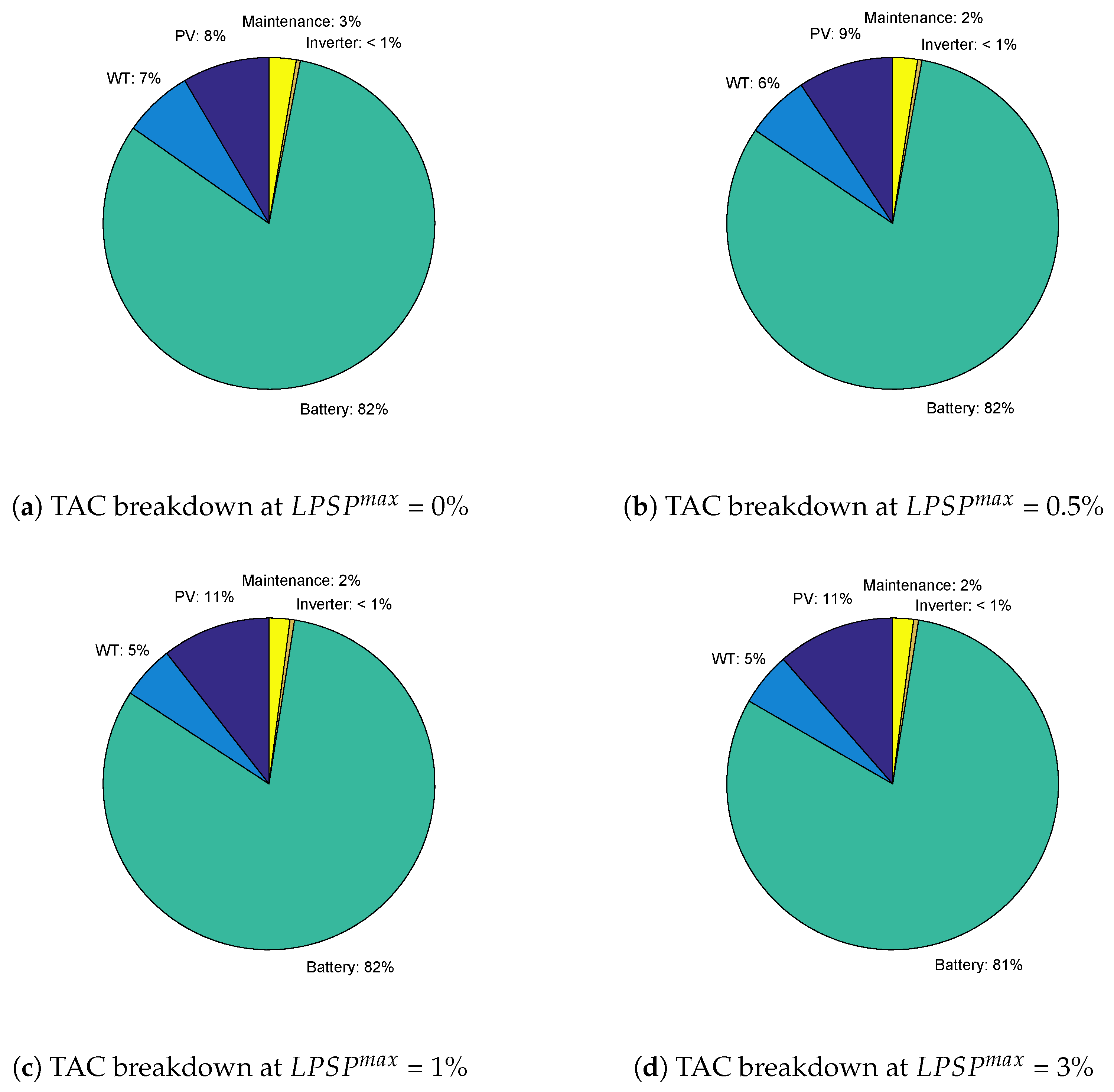
| PV-WT-battery | 0 | 5469 | 4365 | 52,637 | 259 | 1700 | 64,430 | |
| 0.5 | 5764 | 3852 | 50,595 | 259 | 1500 | 61,970 | ||
| 1 | 6257 | 3081 | 48,403 | 259 | 1200 | 59,200 | ||
| 3 | 6208 | 2825 | 43,779 | 259 | 1100 | 54,171 | ||
| System | TLBO | EDE | SSA | EESA | |||||||||||||||||
|---|---|---|---|---|---|---|---|---|---|---|---|---|---|---|---|---|---|---|---|---|---|
| (%) | (%) | TAC ($) | (%) | TAC ($) | (%) | TAC ($) | (%) | TAC ($) | |||||||||||||
| PV-Battery | 0 | 0 | 199 | 0 | 3150 | 104,640 | 0 | 199 | 0 | 3150 | 104,640 | 0 | 200 | 0 | 3200 | 106,200 | 0 | 199 | 0 | 3150 | 104,640 |
| 0.5 | 0.4932 | 194 | 0 | 2898 | 96,840 | 0.4932 | 194 | 0 | 2898 | 96,840 | 0.4932 | 194 | 0 | 2898 | 96,840 | 0.4932 | 194 | 0 | 2898 | 96,840 | |
| 1 | 0.8820 | 191 | 0 | 2746 | 92,120 | 0.7526 | 192 | 0 | 2797 | 93,700 | 0.6160 | 193 | 0 | 2847 | 95,250 | 0.8820 | 191 | 0 | 2746 | 92,120 | |
| 3 | 2.8942 | 178 | 0 | 2090 | 71,790 | 2.8942 | 178 | 0 | 2090 | 71,790 | 2.7459 | 179 | 0 | 2141 | 73,370 | 2.8942 | 178 | 0 | 2090 | 71,790 | |
| Average rank | 91,348 | 91,743 | 92,915 | 91,348 | |||||||||||||||||
| Final rank | 1 | 2 | 3 | 1 | |||||||||||||||||
| System | EESA | |||||||
|---|---|---|---|---|---|---|---|---|
| (%) | Configuration | ($) | ($) | ($) | ($) | ($) | TAC ($) | |
| PV-battery | 0 | 9800 | 0 | 94,580 | 260 | 0 | 10,4640 | |
| 0.5 | 9560 | 0 | 87,020 | 260 | 0 | 96,840 | ||
| 1 | 9410 | 0 | 82,450 | 260 | 0 | 92,120 | ||
| 3 | 8770 | 0 | 62,760 | 260 | 0 | 71,790 | ||
| System | TLBO | EDE | SSA | EESA | |||||||||||||||||
|---|---|---|---|---|---|---|---|---|---|---|---|---|---|---|---|---|---|---|---|---|---|
| (%) | (%) | TAC ($) | (%) | TAC ($) | (%) | TAC ($) | (%) | TAC ($) | |||||||||||||
| PV-Battery | 0 and 0.5 | 0 | 0 | 50 | 3552 | 124,750 | 0 | 0 | 50 | 3552 | 124,750 | 0 | 0 | 50 | 3552 | 124,750 | 0 | 0 | 50 | 3552 | 124,750 |
| 1 and 3 | 0.5503 | 0 | 49 | 3362 | 118,690 | 0.5503 | 0 | 49 | 3362 | 118,690 | 0.5503 | 0 | 49 | 3362 | 118,690 | 0.5503 | 0 | 49 | 3362 | 118,690 | |
| Average rank | 121,720 | 121,720 | 121,720 | 121,720 | |||||||||||||||||
| Final rank | 1 | 1 | 1 | 1 | |||||||||||||||||
| System | EESA | |||||||
|---|---|---|---|---|---|---|---|---|
| (%) | Configuration | ($) | ($) | ($) | ($) | ($) | TAC ($) | |
| WT-Bat. | 0 and 0.5 | 0 | 12,840 | 106,650 | 260 | 5000 | 124,750 | |
| 1 and 3 | 0 | 12,580 | 100,950 | 260 | 4900 | 118,690 | ||
© 2019 by the authors. Licensee MDPI, Basel, Switzerland. This article is an open access article distributed under the terms and conditions of the Creative Commons Attribution (CC BY) license (http://creativecommons.org/licenses/by/4.0/).
Share and Cite
Khan, A.; Alghamdi, T.A.; Khan, Z.A.; Fatima, A.; Abid, S.; Khalid, A.; Javaid, N. Enhanced Evolutionary Sizing Algorithms for Optimal Sizing of a Stand-Alone PV-WT-Battery Hybrid System. Appl. Sci. 2019, 9, 5197. https://doi.org/10.3390/app9235197
Khan A, Alghamdi TA, Khan ZA, Fatima A, Abid S, Khalid A, Javaid N. Enhanced Evolutionary Sizing Algorithms for Optimal Sizing of a Stand-Alone PV-WT-Battery Hybrid System. Applied Sciences. 2019; 9(23):5197. https://doi.org/10.3390/app9235197
Chicago/Turabian StyleKhan, Asif, Turki Ali Alghamdi, Zahoor Ali Khan, Aisha Fatima, Samia Abid, Adia Khalid, and Nadeem Javaid. 2019. "Enhanced Evolutionary Sizing Algorithms for Optimal Sizing of a Stand-Alone PV-WT-Battery Hybrid System" Applied Sciences 9, no. 23: 5197. https://doi.org/10.3390/app9235197
APA StyleKhan, A., Alghamdi, T. A., Khan, Z. A., Fatima, A., Abid, S., Khalid, A., & Javaid, N. (2019). Enhanced Evolutionary Sizing Algorithms for Optimal Sizing of a Stand-Alone PV-WT-Battery Hybrid System. Applied Sciences, 9(23), 5197. https://doi.org/10.3390/app9235197