Study of Orientation Error on Robot End Effector and Volumetric Error of Articulated Robot

Featured Application

Calibration of industrial robot and multi-link system.

Abstract

Robots are being used in many areas. The robot performance constraints are repeatability and accuracy. Standardized testing and evaluation techniques are needed to examine the process capability of a wide variety of robots. Robot calibration is a term applied to the procedure used in determining actual values which describe the geometric dimensions and mechanical characteristics of a robot. The robot accuracy evaluation method is introduced. The study proposed a technique to analyze robot’s orientation error by using the data measured during circle contouring movement of the articulated robot end effectors. New measuring method is proposed to measure orientation errors. Circle contouring measurements were also undertaken to assess the significance of multi-axis movements on the accuracy of the end effector. The paper describes the experimental and theoretical accuracy characteristics of an articulated robot. Also, the technique devised using a simulation program for the robot geometry, together with results from a circular test, enables robot errors to be characterized in terms of orientation error and volumetric error. Close correlation was obtained between the experimental and theoretical results. Also, robot pose error was shown a significant factor influencing the accuracy of the robot end effector. Proposed techniques are useful to set up the articulated robot in the industrial site.

1. Introduction

Articulated robots are being used in many areas where accuracy and kinematic performance can be crucial, for example in part assembly, drilling, deburring, and welding. These operations require performance that was needed on robot system. The major robot performance constraints are repeatability and accuracy, following by uptime, load capacity, velocity, and size of robot. The specifications quoted by the manufacturers, are generally not sufficient to determine the process capability of the robot required. Most of the time, manufacturers specify resolution, repeatability, and accuracy rather than pose, but pose is important for offline programming and process planning. Robots from the same production batch, with identical specifications, can demonstrate different characteristics when operated under different conditions (different loads, speeds, durations, temperature, etc.). Standardized testing and evaluation techniques are needed to examine the process capability of a wide variety of robots in order to make the appropriate selection [1,2,3,4,5,6,7]. During their life robots may require maintenance which may involve changing encoders etc. Unless a re-datuming technique is available then the accuracy could differ significantly from that achieved prior to the maintenance. To achieve the previous performance, re-teaching or re-datuming may be required [8,9].

When the robot parameter does not coincide with the designer’s intention, the error occurs between the taught position and the design data-based position. If the control parameter set up in the initial stage is applied to the robot hardware exactly, the robot system becomes a new one in accuracy perspective. To control the end effectors of an articulated robot to intended locations in general, controller for each driving axis are calculated based on modeling parameter. Therefore, the end effectors deviate from the expected position to have position and pose error when the actual kinematic parameter has error. The accuracy of an industrial robot can be improved through calibration [10,11,12].

There are two ways to address the position error of the robot. One is using the sensor and control technology and the other is calculating the robot parameter through measurement before modifying the control parameter of the controller.

The first step is to choose the mathematical model that will improve the representation of the position and orientation of the robot end-effector. This mathematical model is a function of the robot joint angles and takes into account the error parameters that need to be modeled.

The error parameters can be identified by measuring the complete pose or partial pose of the robot end-effector in a set of calibration robot configurations. Many measurement devices have been used for robot calibration or validation, such as: A touch probe and a reference artifact [13], a telescoping ball bar [14], a small-range 3D position measurement device such as a camera-based system, [15] acoustic sensors [16], a large-range 3D measurement device such as a laser tracker [17,18,19], and a 6D complete pose measurement device such as a camera-based system. [20]

The robot parameter is calibrated to reduce the robot teaching time, failure cost, and operating the robot system efficiently as required works are increasingly diverse and complicated. Offline teaching can be done on a separate work area or the computer simulation result can be used for the robot rather instead of direct teaching. In other words, accurate robot system and exact geometric information of the target to work on is enough under offline program to efficiently produce an operation program for multiple robots and this can prevent malfunctioning and conflict during operation of the robot system. However, calibration of inaccurate robot parameters is needed to apply the offline programming to the industry. The parameters are used to build system model of the robot and work subject on the computer for the offline program and kinematic relationship.

Geometric errors in robots, i.e., errors in joint angles and datum location error, are considered to be the main sources of position error [8,21]. The repeatability errors are non-geometric; these include gear transmission error, joint drive compliance, backlash, bearing, and encoder inaccuracy. Other sources of robot inaccuracy include link geometry errors, elastic deflection, scale and control errors, and environmental effects.

Consequently, a new system using a six-point kinematic design was developed by the author for measuring the orientation error and tested on the industrial robot because a six-point kinematic design can attain good repeatability and has good rigidity. The aim of this research is to develop a strategy for the robot pose evaluation of industrial robots by using low-cost hardware in the form of ball bars. A new design for the kinematic system will be investigated in order to overcome orientation measurement limitation with existing systems. The problem of interpretation of the data obtained from the new hardware will be investigated by simulating the kinematic model of the robot structure for six degrees of freedom and comparing these with the experimental data obtained using this new hardware. The experimental verification of the strategy will be undertaken on a standard six axes industrial robot and the effect of orientation errors on the kinematics is theoretically simulated and analyzed.

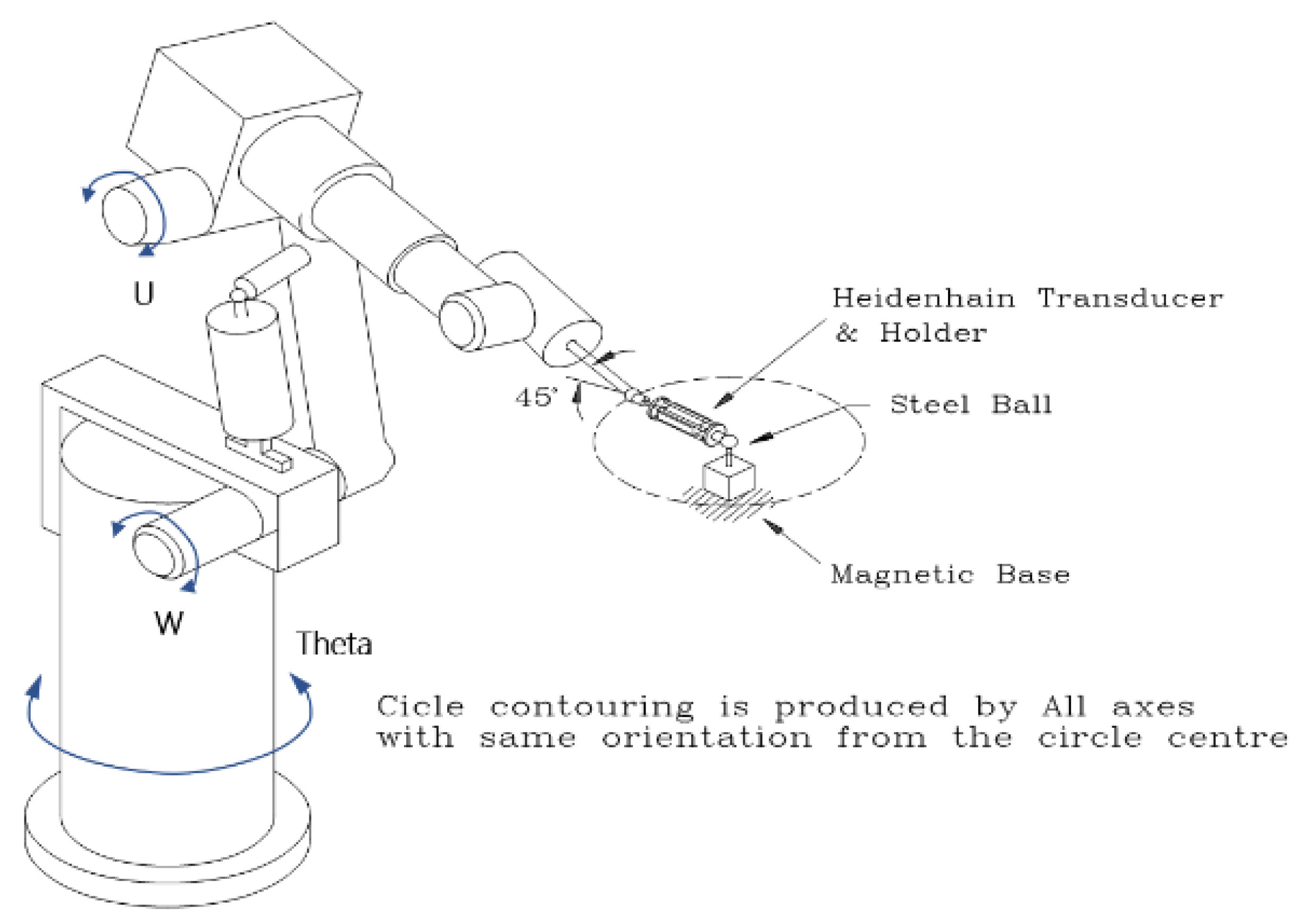
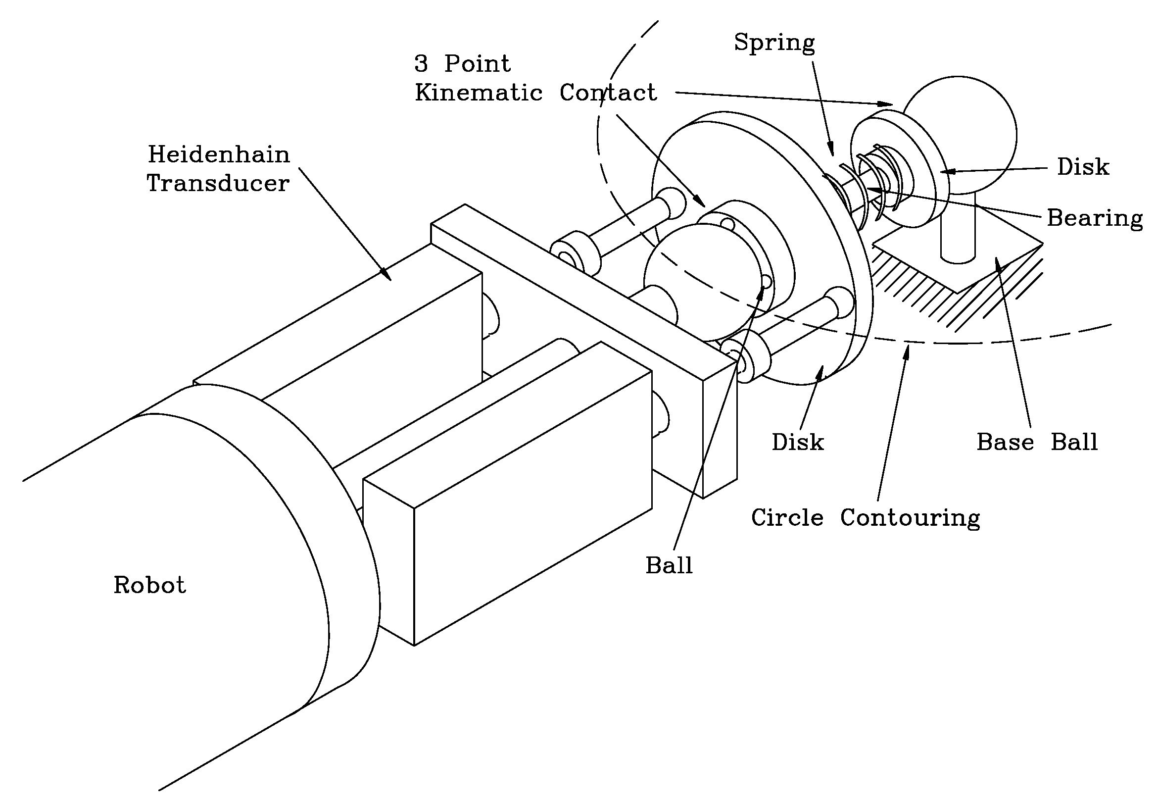
2. Orientation Test of Robot End Effector

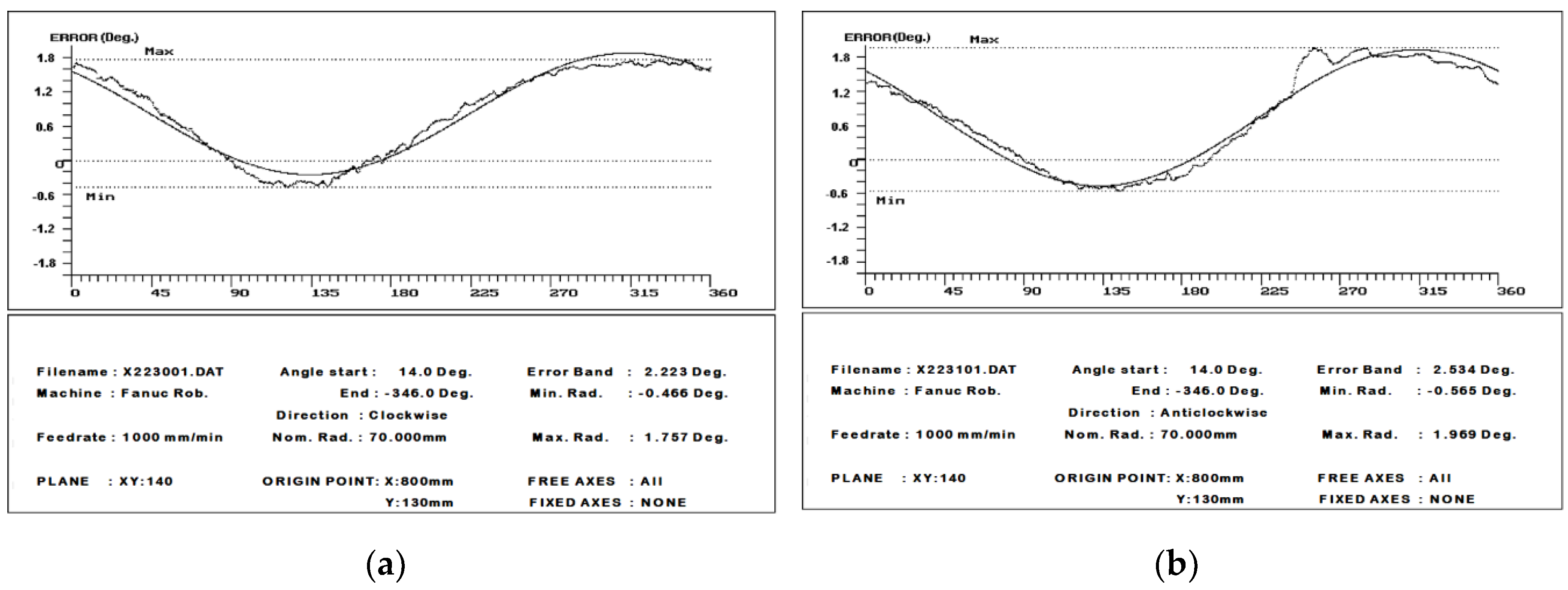
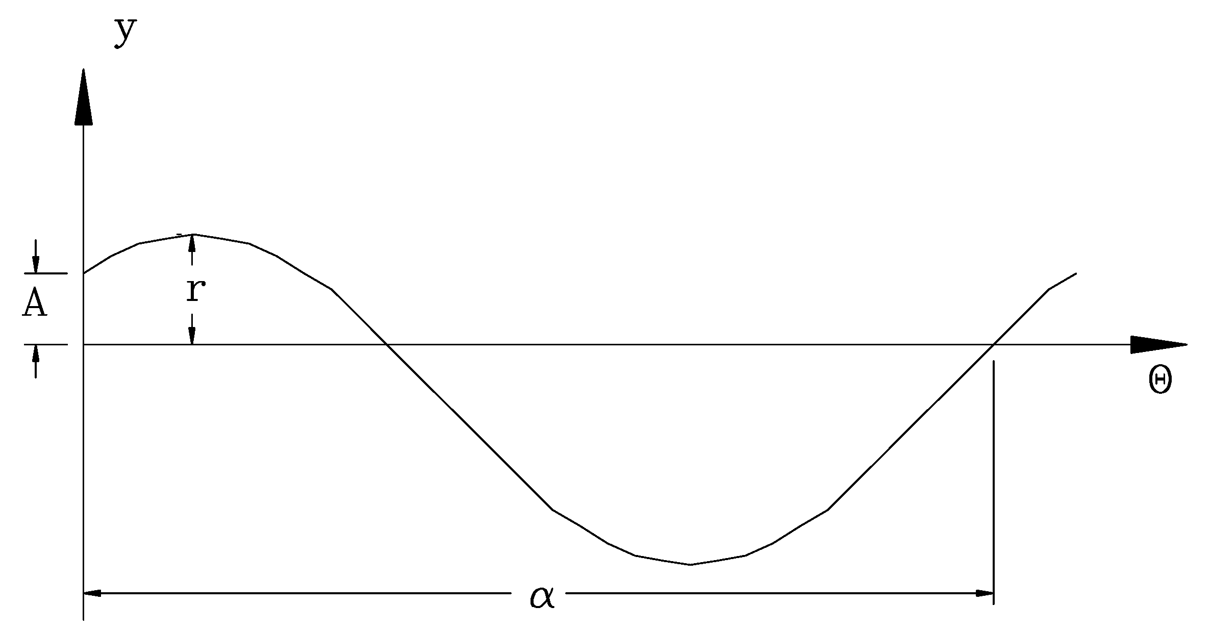
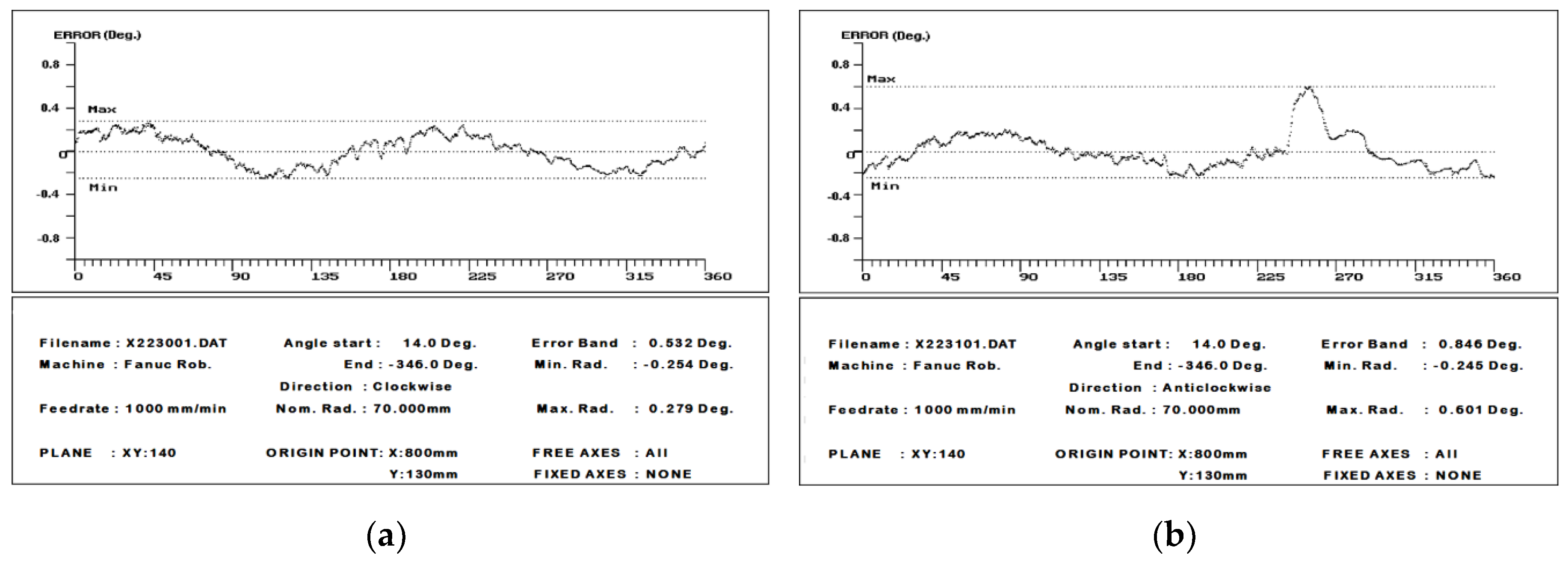
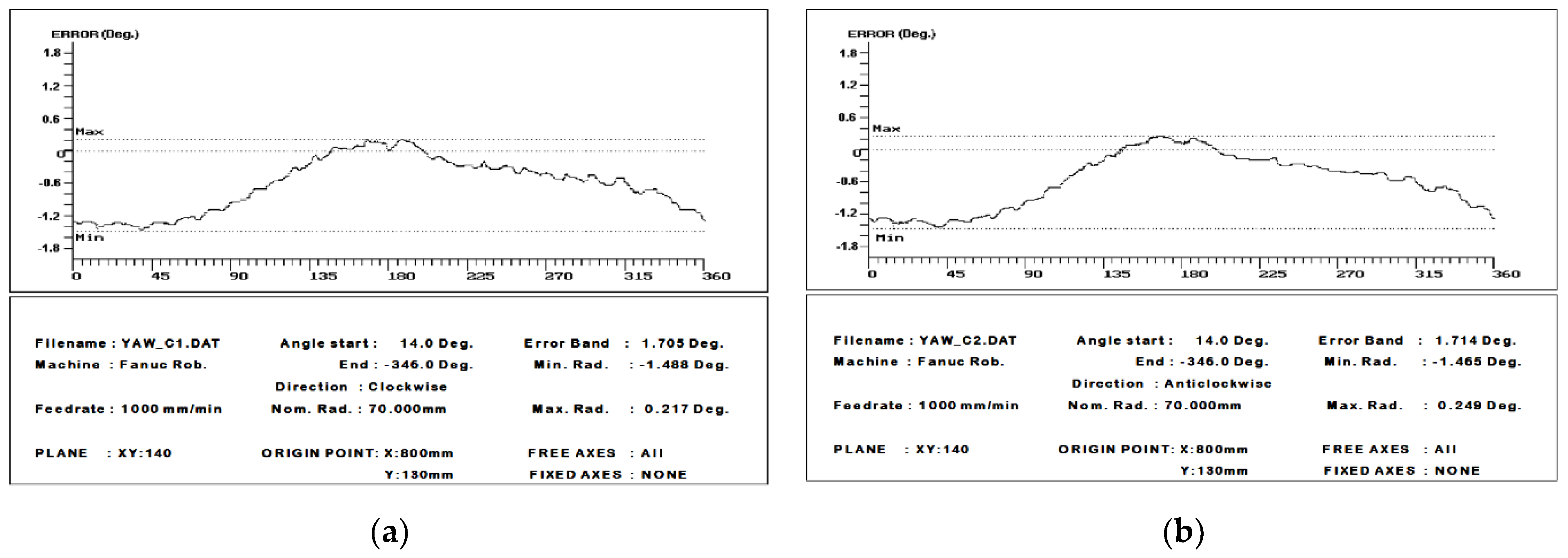
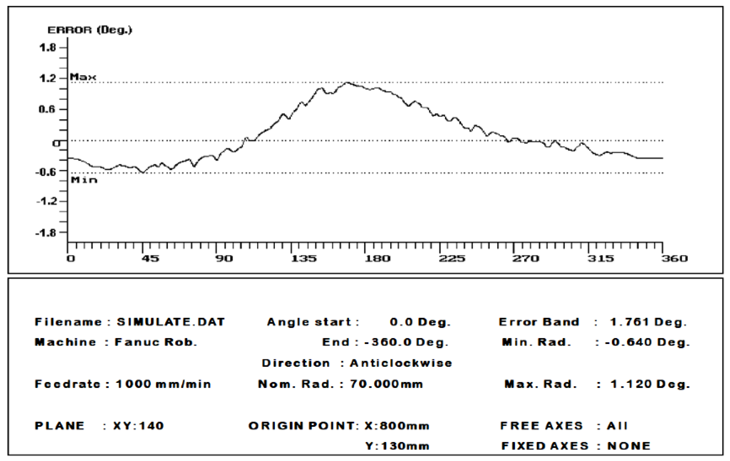
2.1. Orientation Test of Yaw Motion in the Robot End Effector

When the robot generated the circular contouring using the main three axes, i.e., Theta W and U axes, only the position of the end effector is controlled, and the orientation of end effector is constantly changing from the center of the circle. During the six axes operation, the robot was able to control precisely both the position and orientation of the robot end effector as shown in Figure 1. To measure the orientation and position of the robot end effector simultaneously is difficult due to the limitations of the robot working space, and transducer length. Achieving a robot end effector whose position pose is parallel to the XY plane, is limited to a maximum circle radius of 70 mm.

Special equipment was made using a six points kinematic concept to measure the yaw motion of the robot end effector as shown Figure 2. Three small balls at angular spacing of 120° were fixed to faces of two circular disks. A linear bearing was fixed onto one of the circular disks to facilitate a sliding motion between the disks and positive contact maintained between the measurement spheres by a spring force. Two transducers, which touch on the first circular disk, are mounted at the robot end effector; the distance between the two transducers being set to 50 mm.

The equipment is self-supporting by the spring force between the base-ball and the end effector as shown in Figure 2. The difference value of the two transducers was measured whilst the robot operated in a manner to maintain constant orientation in the radial direction during the circular contouring. The yaw motion angle error of the orientation was calculated from this difference value between the two transducers.

Figure 3a,b show the results in both the clockwise and anticlockwise directions and the error shape displays a sine curve function. This shape results from an eccentric setting between the center of the base-ball and the center of the circular contouring. This eccentricity situation is shown in Figure 4. If the base-ball is located at the center of the circle, and there is no yaw motion error in the robot axes, the circular disk is always square to the robot end effector during the robot generated circular contouring, in the radial direction.

If eccentricity between the center of the base-ball and the circle exists, then the error shape is a sine curve function [22], as shown in Figure 3. The amplitude of the sine curve is a function of the magnitude of eccentricity and the circle radius. For circle contouring with a radius R, the amplitude of sine curve error E based on the its eccentricity is [23].

$$E_{max}\left[arcsec\right]=\pm 206·e\left[\mu m\right]/R\left[mm\right]$$

where e is the eccentricity between the center of the base-ball and the circle.

Depending on the 70 mm radius of the circular contouring, an eccentricity of 14.142 mm results in measuring deviation of ±11.56 degrees as shown in Figure 4. Figure 4 shows the angle error due to eccentricity, and the resultant error is seen to be a sine curve.

Therefore, the experimental sine curve wave seen in Figure 3a,b is due to eccentricity. The least squares sine curve was calculated and also plotted in Figure 3a,b. The equation of least squares sin curve is shown in the below.

Assume that in the Figure 5

$$y_k=A+r\sin \left({\theta }_k+\alpha \right),$$

(1)

where, r: Amplitude, A: Offset of amplitude, α: Shift-angle, and θ_k: Rotation-angle.

According to least squares definition

$$E\left(y\right)={\displaystyle \sum _{k=1}^m{\left[A+r\sin \left({\theta }_k+\alpha \right)-y_k\right]}^2},$$

(2)

is minimized.

To illustrate least squares error approximation, consider the important problem of fitting a sin curve. This guess function for this rather special fit will be denoted by

$$\begin{array}{ll}E\left(y\right)& ={\displaystyle \sum _{k=1}^m{\left[A+r\sin \left({\theta }_k+\alpha \right)-y_k\right]}^2}\\ & ={\left[A+r\sin \left({\theta }_1+\alpha \right)-y_1\right]}^2+\cdot \cdot \cdot +{\left[A+r\sin \left({\theta }_m+\alpha \right)-y_m\right]}^2\end{array}$$

(3)

But

$$\begin{array}{ll}{y}_k& =A+r\sin \left({\theta }_k+\alpha \right)\\ & =A+\left[\left(r\cos \alpha \right)\sin {\theta }_k+r\sin \alpha \cos {\theta }_k\right]\\ & =A+a\sin {\theta }_k+b\cos {\theta }_k\end{array}$$

(4)

Let $r\cos \alpha =a$ $r\sin \alpha =b$

i.e.,

$$E\left(y\right)={\displaystyle \sum _{k=1}^m{\left[A+a\sin {\theta }_k+b\cos {\theta }_k-y_k\right]}^2}$$

We know from calculus that this will occur when

$$\begin{gathered} \frac{\partial E\left(y\right)}{\partial A}=0 \\ ,\frac{\partial E\left(y\right)}{\partial a}=0,\frac{\partial E\left(y\right)}{\partial b}=0 \\ \frac{\partial E\left(y\right)}{\partial A}=2{\displaystyle \sum _{k=1}^m\left(A+a\sin {\theta }_k+b\cos {\theta }_k-y_k\right)}=0, \end{gathered}$$

(5)

$$\frac{\partial E\left(y\right)}{\partial a}=2{\displaystyle \sum _{k=1}^m\left[A\sin {\theta }_k+a{\sin }^2{\theta }_k+b\cos {\theta }_k\sin {\theta }_k-y_k\sin {\theta }_k\right]}=0,$$

(6)

$$\frac{\partial E\left(y\right)}{\partial b}=2{\displaystyle \sum _{k=1}^m\left[A\cos {\theta }_k+a\sin {\theta }_k\cos {\theta }_k+b{\cos }^2{\theta }_k-y_k\cos {\theta }_k\right]}=0,$$

(7)

From the Equations (5–7)

$$\left|\begin{array}{ccc}m& {\displaystyle \sum \sin {\theta }_k}& {\displaystyle \sum \cos {\theta }_k}\\ {\displaystyle \sum \sin {\theta }_k}& {\displaystyle \sum {\sin }^2{\theta }_k}& {\displaystyle \sum \cos {\theta }_k\sin {\theta }_k}\\ {\displaystyle \sum \cos {\theta }_k}& {\displaystyle \sum \sin {\theta }_k\cos {\theta }_k}& {\displaystyle \sum {\cos }^2{\theta }_k}\end{array}\right|\left|\begin{array}{c}A\\ a\\ b\end{array}\right|=\left|\begin{array}{c}{\displaystyle \sum y_k}\\ {\displaystyle \sum y_k\sin {\theta }_k}\\ {\displaystyle \sum y_k\cos {\theta }_k}\end{array}\right|,$$

(8)

$$\left|\begin{array}{c}A\\ a\\ b\end{array}\right|=\frac{1}{\det \left(Q\right)}\left|\begin{array}{ccc}{b}_{11}& b_{12}& b_{13}\\ b_{21}& b_{22}& b_{23}\\ b_{31}& b_{32}& b_{33}\end{array}\right|\left|\begin{array}{c}{\displaystyle \sum y_k}\\ {\displaystyle \sum y_k\sin {\theta }_k}\\ {\displaystyle \sum y_k\cos {\theta }_k}\end{array}\right|,$$

(9)

$$\begin{array}{l}A=\frac{1}{\det \left(Q\right)}\left(b_{11}{\displaystyle \sum y_k+b_{12}{\displaystyle \sum y_k\sin {\theta }_k+b_{13}{\displaystyle \sum y_k\cos {\theta }_k}}}\right)\\ a=\frac{1}{\det \left(Q\right)}\left(b_{21}{\displaystyle \sum y_k+b_{22}{\displaystyle \sum y_k\sin {\theta }_k+b_{23}{\displaystyle \sum y_k\cos {\theta }_k}}}\right)\\ b=\frac{1}{\det \left(Q\right)}\left(b_{31}{\displaystyle \sum y_k+b_{32}{\displaystyle \sum y_k\sin {\theta }_k+b_{33}{\displaystyle \sum y_k\cos {\theta }_k}}}\right)\end{array},$$

(10)

From the Equation (1)

$$\begin{array}{ll}{y}_k& =A+a\sin \theta +b\cos \theta \\ & =A+r\sin \left(\theta +\alpha \right)\end{array},$$

(11)

where

$$\begin{gathered} r=\sqrt{a^2+b^2}\hspace{1em}\alpha ={\tan }^{-1}\left(\frac{b}{a}\right) \\ r=\frac{1}{\det \left(Q\right)}\sqrt{{\left(b_{21}{\displaystyle \sum y_k+b_{22}{\displaystyle \sum y_k\sin {\theta }_k+b_{23}{\displaystyle \sum y_k\cos {\theta }_k}}}\right)}^2+{\left(b_{31}{\displaystyle \sum y_k+b_{32}{\displaystyle \sum y_k\sin {\theta }_k+b_{33}{\displaystyle \sum y_k\cos {\theta }_k}}}\right)}^2} \\ \alpha ={\tan }^{-1}\left(\frac{b_{31}{\displaystyle \sum y_k+b_{32}{\displaystyle \sum y_k\sin {\theta }_k+b_{33}{\displaystyle \sum y_k\cos {\theta }_k}}}}{b_{11}{\displaystyle \sum y_k+b_{22}{\displaystyle \sum y_k\sin {\theta }_k+b_{23}{\displaystyle \sum y_k\cos {\theta }_k}}}}\right) \end{gathered}$$

The deviations between the real data and least squares sine curve are real orientation errors of yaw motion in the robot end effector, as shown Figure 6a,b. The error band is about 0.53° in the clockwise direction and 0.85° anticlockwise. The error shape is slightly different due to the backlash error of the robot axes. The fluctuation of the error is due to the gear transmission error of the robot axes.

The angle change of the robot axes is found with the inverse kinematic solution for the robot generated circular contouring. Figure 7 shows this angle change during the circular contouring. All the robot axes, except the gamma axis, show inflexion points during the circle contouring. The backlash points occur at the direction change of the angle in each axes. The rectangular mark shows the direction change point in Figure 7. If backlash exists in the robot axes, then angle error will suddenly be apparent during the robot operation.

The simulation result of the circle contouring is shown in Figure 8a,b. The simulation procedure is the same as mentioned [24]. The X, Y, and Z positions to make the theoretical circle contouring in the robot working space is calculated and input into the inverse kinematic solution program, and then the corresponding angles of the W and U axes are found i.e., the X, Y, and Z positions in the robot working space correspond to the angles of the W and U axes. The calculated angles and the datum location error of the gamma and beta axes were input in the kinematic solution. The result of this computation gives the X, Y, and Z positions of the robot with the influence of the datum location error of the gamma and beta axes. For comparison with the experimental results the circle radius and error band were evaluated. Figure 8a shows orientation error of yaw motion in the clockwise direction. Figure 8b shows the same in the anticlockwise direction. Comparing Figure 8a,b, the error tendency is slightly different due to the backlash of the robot axes. The sudden change is due to the backlash of the theta axes at 237°.

Table 1. Direction change of robot axes angle during circle contouring.

Robot Axes	Upper Backlash Point	Lower Backlash Point
Theta	105°	237°
W	3°	182°
U	351°	169°
Beta	0°	190°
Alpha	82°	290°

is shown the backlash point during circulation.

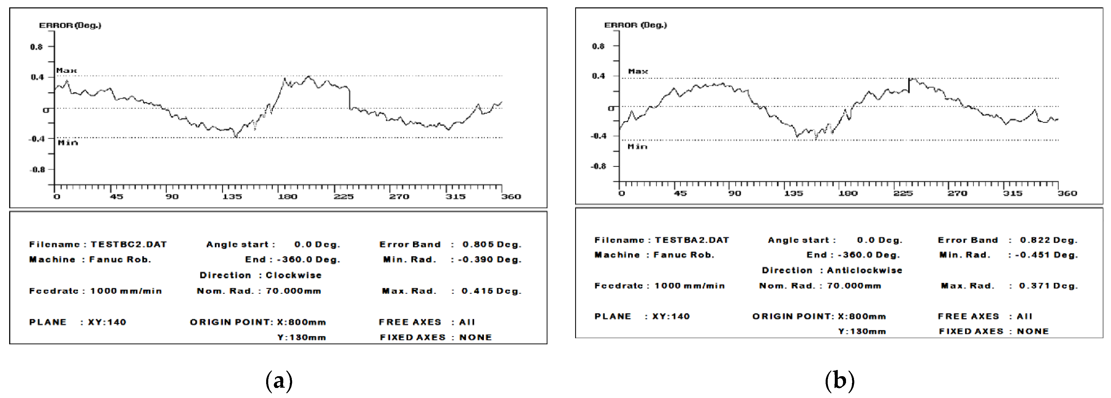
2.2. Orientation Test of Roll Motion in the Robot end Effector

Figure 9 shows the equipment setting for the orientation test of the roll motion. The defined positions and orientation of the robot end effector for the circular contouring are the same as the yaw test position. The difference is that the transducer is rotated by 90 degrees from the position of the yaw motion test. The results are shown in Figure 10a,b in both clockwise and anticlockwise directions. Comparing the two graphs in Figure 10a,b, the error shapes are almost identical. Therefore, backlash error has no influence on the roll motion error in the robot axes. If the gear transmission error and backlash error of the robot axes were negligible, the error shape would be a straight line, i.e., the error band would be zero degrees. However, the error band has a value of approximately 1.75 degrees which stems mainly from the gear transmission error in the robot axes.

The simulation result for the same test is shown in Figure 11. The error band is about 1.76 degree. The error curve shows maximum and minimum points around 180 and 45 degrees on the circle. The simulation error shape and band are very similar to the experimental data.

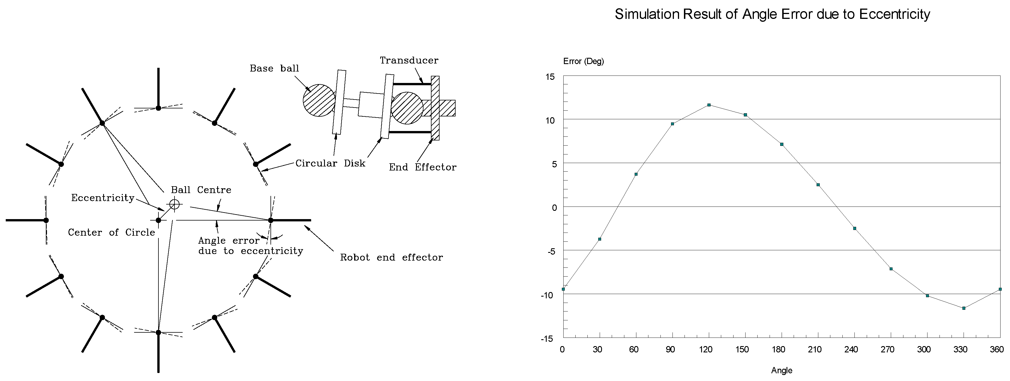
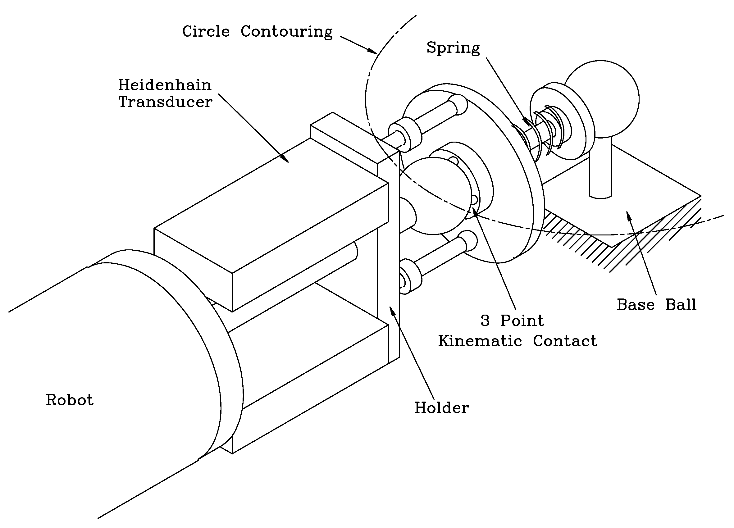
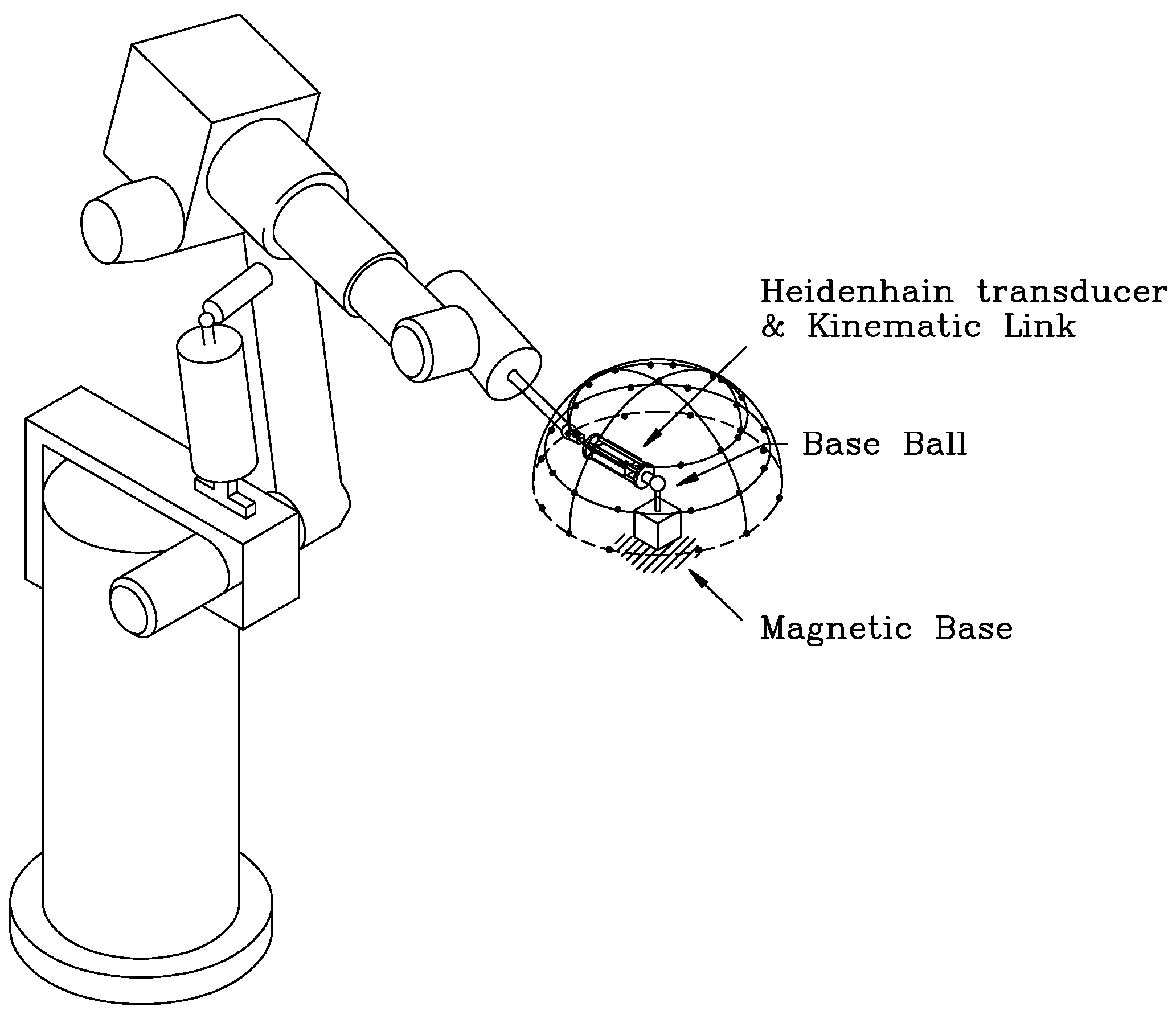
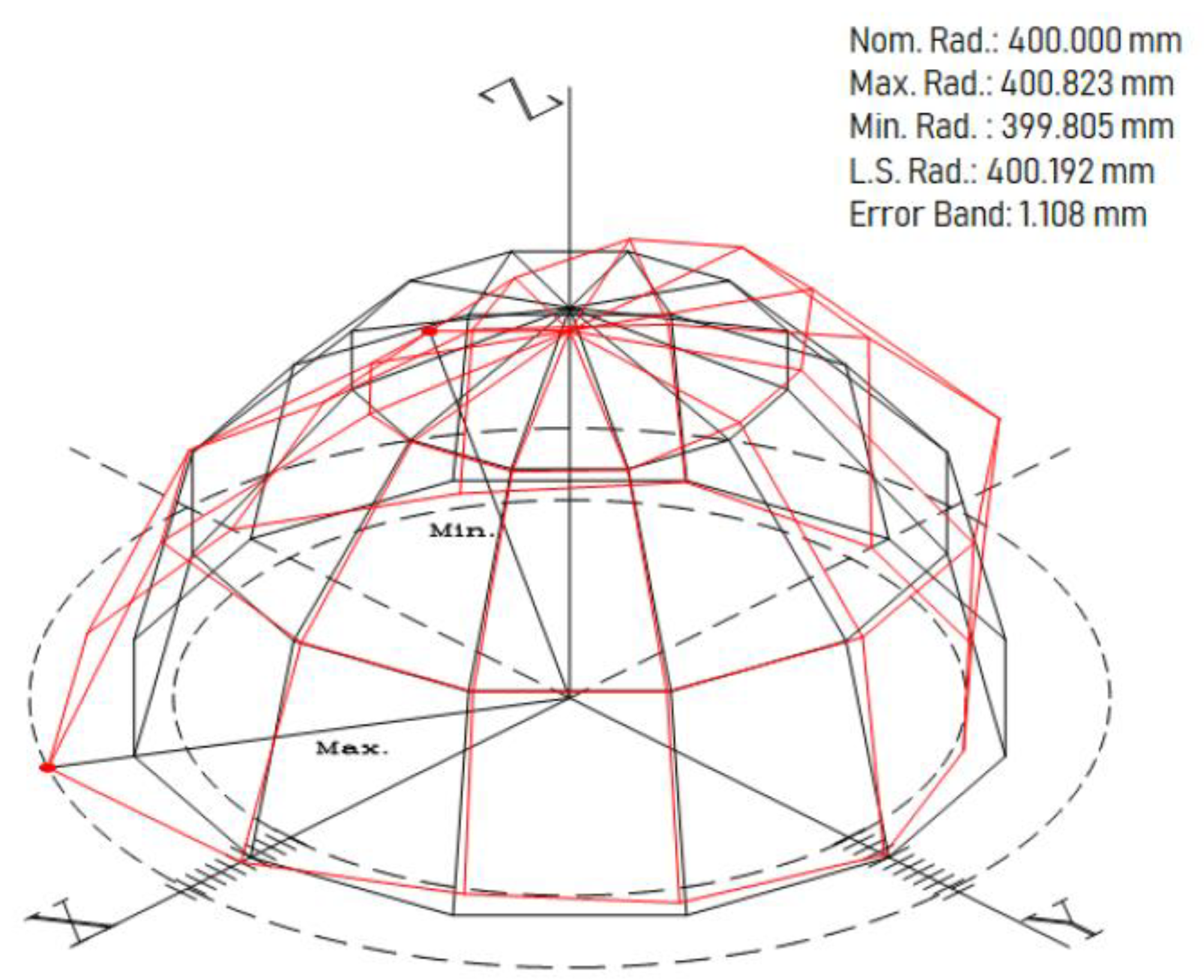
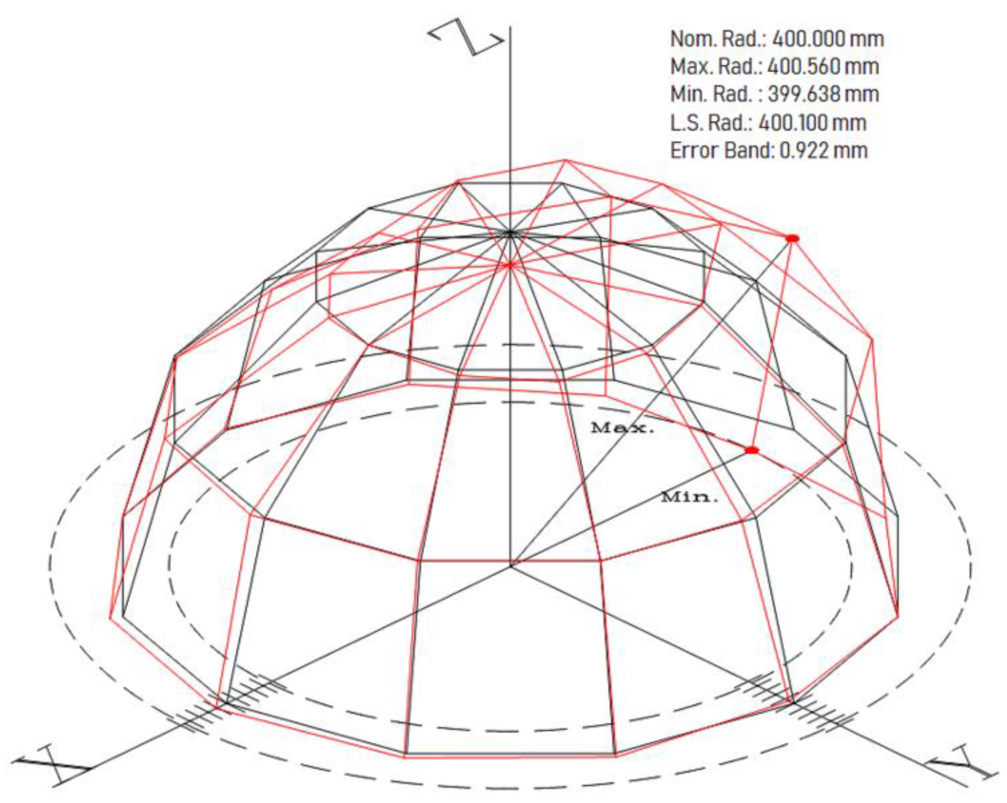
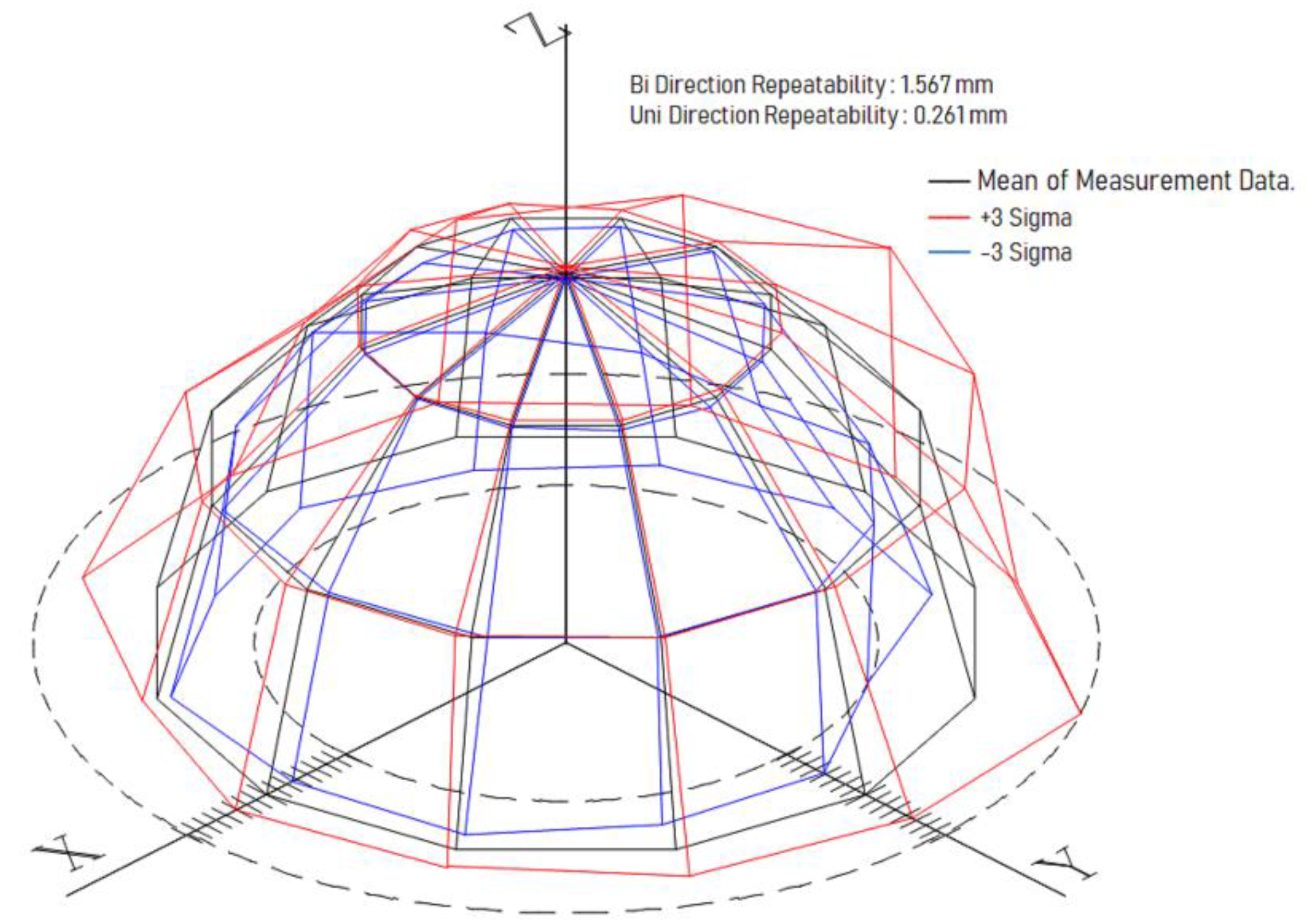
2.3. Radial Position Accuracy and Repeatability Test on a Hemisphere

The positional accuracy of the robot at different orientations of the robot end effector, is tested on a hemisphere of 400 mm radius as defined and shown in Figure 12. The target positions are equivalent to 30 degree intervals on the hemisphere. Each of the target positions is defined by three different orientations of robot end effector at the same position of the robot end effector. The equipment setting and target positions are shown in Figure 12. The radial distance between the target position of the end effector and the base-ball was measured using a transducer and kinematic link at the different orientations.

The experimental results are shown in the Figure 13. The experimental result, which is red color in the figure, are the mean value of the three different orientations at the same position of the robot end effector. The least squares sphere, which is black color on the Figure 13, is calculated from the experimental mean value using the least squares approximation method. The nominal radius is 400 mm, but the radius of the least squares sphere is 400.192 mm. The error band is seen to be just greater than 1 mm. The experimental data can also be seen to be distorted to one side when compared with the least squares sphere.

The target angle positions of each of axes were found with the inverse kinematic solution. The gear transmission error of each of the axes is added to the theoretical target angle positions of each of the axes. The distance between the center of the hemisphere and the position of the end effector was calculated for these simulation results as shown in Figure 14. The radius of the least squares sphere is again larger than the nominal radius, and the error band just less than 1 mm at 0.922 mm. Again, the simulation data is distorted to one side when compared with the least squares sphere. Compared with the experimental result, the error tendency of the simulation data is almost identical. This distortion is due therefore to the gear transmission error and backlash of the robot axes since these are the only correction made to the simulation data.

To test repeatability, the end effector is approached to the target position, and the distance between the two balls was measured with a transducer and kinematic link. The end effector is then moved to a position, which is in the same radial direction, but at a 3 mm greater nominal radius, then the end effector is returned to the target position in the same radial direction. The distance between two balls is again measured. Then the end effector is moved to a position, in the radial direction, which is 3 mm smaller than the nominal radius, and again the end effector returned to the target position in the same radial direction. The distance between the two balls is again measured. This procedure is repeated three times and six measurement data are acquired from one target point. The result of this repeatability test is shown in Figure 15. The uni-direction repeatability is found to be 0.261 mm, the bi-direction repeatability shows 1.567 mm. The bi-direction repeatability is seven times larger than uni-direction repeatability due to the backlash error of the theta and beta robot axes.

3. Conclusions

The following conclusions can be drawn from the investigation on robot accuracy. A new type of kinematic ball link system was designed and tested. This incorporated three points contact between the sockets and the balls and utilized the magnetic force in the socket to locate the link between the reference balls. This new design proved to be successful in operation and provided the following advantages over existing ball bars. This link system is light weight and low cost compare with existing system such as a camera-based system and a laser tracker. Also, the existing system is limited to the measuring area of sensor, and it can measure some working areas when the robot movies in a circle. However, the link system has the advantage of measuring the whole working area of the robot. The accuracy and the repeatability of the link depends mainly on the digital transducer which has a repeatability of 0.5 μm. The absolute length of the link can be determined precisely by means of a calibrated setting fixture. The performance of the link over the period of the research has shown that it was sufficiently robust for application to robots operating in industrial environments.

Parametric error components of industrial robots are generally difficult to establish compared with the orthogonal linear axes of machine tools. The research has shown that the techniques devised using basic equipment such as an extended range of ball links, together with a sensitive angular instrument such as a linear transducer, can be successfully applied to establish the orientation and volumetric error. The technique devised using a simulation program for the robot geometry, together with results from a circular test, enables robot errors to be characterized in terms of robot pose error such as roll, pitch, and volumetric characteristics. Circular test data is a valuable technique for characteristic the robot error in terms of robot orientation error and volumetric error etc. The robot orientation error due to robot parametric error. Also, robot pose error was shown a significant factor influencing the accuracy of the robot end effector. Proposed techniques are useful to set up the articulated robot in the industrial site.

References

1. Brussel, H.V. Evaluation and testing of robots. CIRP Annals-Manufacturing Technology 1990, 39, 657–664. [Google Scholar] [CrossRef]
2. Lau, K.; Hocken, J.A. Survey of current robot metrology methods. CIRP Annals-Manufacturing Technology 1984, 32, 485–488. [Google Scholar] [CrossRef]
3. Warnecke, H.J.; Weck, M.; Brodbeck, B.; Engel, G. Assessment of industrial robots. CIRP Annals-manufacturing Technology 1980, 29, 391–396. [Google Scholar] [CrossRef]
4. Chen, H.; Fuhlbrigge, T.; Choi, S.; Wang, J.; Li, X. Practical industrial robot zero offset calibration. In Proceedings of the 2008 IEEE International Conference on Automation Science and Engineering, Piscataway, NJ, USA, 23–26 Augst 2018; pp. 516–521. [Google Scholar]
5. Lei, S.; Jingtai, L.; Weiwei, S.; Shuihua, W.; Xingbo, H. Geometry-based robot calibration method. In Proceedings of the 2004 IEEE International Conference on Robotics and Automation, ICRA ’04, New Orleans, LA, USA, 26 April–1 May 2004; pp. 1907–1912. [Google Scholar]
6. Nubiola, A.; Bonev, I.A. Absolute Robot Calibration with Single Telescoping Ballbar. Precis. Eng. 2014, 38, 472–480. [Google Scholar] [CrossRef]
7. Nguyen, H.N.; Zhou, J.; Kang, H.J. A new full pose measurement method for robot calibration. Sensors 2013, 13, 9132–9147. [Google Scholar] [CrossRef]
8. Oh, Y.T. Robot accuracy evaluation using a ball-bar link system. Robotica 2011, 29, 917–927. [Google Scholar] [CrossRef]
9. Oh, Y.T. Robot accuracy evaluation using a ball-bar link system. Int. J. Eng. Technol. (IJET) 2015, 7, 833–843. [Google Scholar] [CrossRef]
10. Roth, Z.V.I.S.; Mooring, B.; Ravani, B. An overview of robot calibration. IEEE J. Robot. Autom. 1987, 3, 377–385. [Google Scholar] [CrossRef]
11. Ginani, L.S.; Motta, J.M.S.T. Theoretical and practical aspects of robot calibration with experimental verification. J. Braz. Soc. Mech. Sci. Eng. 2011, 33, 15–21. [Google Scholar] [CrossRef]
12. Dumas, C.; Caro, S.; Cherif, M.; Garnier, S.; Furet, B. A methodology for joint stiffness identification of serial robots. In Proceedings of the IEEE/RSJ International Conference on Intelligent Robots and Systems, Taipei, Taiwan, 18–22 October 2010. [Google Scholar]
13. Khalil, W.; Besnard, S. Geometric calibration of robots with flexible joints and links. J. Intell. Robot. Syst. 2002, 34, 357–379. [Google Scholar] [CrossRef]
14. Ota, H.; Shibukawa, T.; Tooyama, T.; Uchiyama, M. Forward kinematic calibration and gravity compensation for parallel-mechanism-based machine tools. Proc. Inst. Mech. Eng. Part K J. Multi Body Dyn. 2002, 216, 39–49. [Google Scholar] [CrossRef]
15. Beyer, L.; Wulfsberg, J. Practical robot calibration with ROSY. Robotica 2004, 22, 505–512. [Google Scholar] [CrossRef]
16. Stone, H.; Sanderson, A. A prototype arm signature identification system. In Proceedings of the IEEE International Conference on Robotics and Automation, Raleigh, NC, USA, 31 March–3 April 1987. [Google Scholar]
17. Nubiola, A.; Slamani, M.; Joubair, A.; Bonev, I.A. Comparison of two calibration meth-ods for a small industrial robot based on an optical CMM and a laser tracker. Robot. 2013, 32, 447–466. [Google Scholar] [CrossRef]
18. Nubiola, A.; Bonev, I.A. Absolute calibration of an ABB IRB 1600 robot using a laser tracker. Robot. Comput. Integr. Manuf. Robot 2013, 29, 236–245. [Google Scholar] [CrossRef]
19. Umetsu, K.; Furutnani, R.; Osawa, S.; Takatsuji, T.; Kurosawa, T. Geometric calibration of a coordinate measuring machine using a laser tracking system. Meas. Sci. Technol. 2005, 15. [Google Scholar] [CrossRef]
20. Meng, Y.; Zhuang, H. Self-calibration of camera-equipped robot manipulators. Int. J. Robot Res. 2001, 20, 909–921. [Google Scholar] [CrossRef]
21. Yeon Taek, O.H. Influence of the joint angular characteristics on accuracy of industrial robot. Ind. Robot Int. J. 2011, 38, 406–418. [Google Scholar] [CrossRef]
22. Evans, J.C.; Taylerson, C.O. Measurement of Angle in Engineering; Her Majesty’s Stationery Office: London, UK, 1986. [Google Scholar]
23. Warnecke, H.J.; Schiele, G. Performance characteristics and performance testing industrial robot-state of art. In Proceedings of the 1st Robotics and Europe Conference, Brussels, Belgium; 1984; pp. 5–7. [Google Scholar]
24. Yeon Taek, O.H. Evaluation of the Accuracy Performance of Industrial Robot. Ph.D. Thesis, UMIST, Manchester, UK, 1997. [Google Scholar]
Figure 1. Configuration of circular contouring using six axes of articulated robot.
Applsci 09 05149 g001
Figure 2. Equipment setting for the yaw motion test.
Applsci 09 05149 g002
Figure 3. Experimental result of yaw motion test: (a) clockwise direction and (b) anticlockwise direction.
Applsci 09 05149 g003
Figure 4. The angle error due to eccentricity.
Applsci 09 05149 g004
Figure 5. Least square error approximation—curve fitting for sine error curve.
Applsci 09 05149 g005
Figure 6. Experimental data of orientation error in the yaw motion: (a) clockwise direction and (b) anticlockwise direction.
Applsci 09 05149 g006
Figure 7. Angle change of robot axes during circle contouring.
Applsci 09 05149 g007
Figure 8. Simulation result of orientation error in the yaw motion: (a) clockwise direction and (b) anticlockwise direction.
Applsci 09 05149 g008
Figure 9. Equipment setting for roll motion test.
Applsci 09 05149 g009
Figure 10. Experimental data of orientation error in the roll motion: (a) clockwise direction and (b) anticlockwise direction.
Applsci 09 05149 g010
Figure 11. Simulation result of orientation error in the roll motion.
Applsci 09 05149 g011
Figure 12. Equipment setting and defined position.
Applsci 09 05149 g012
Figure 13. Experimental result of radial accuracy.
Applsci 09 05149 g013
Figure 14. Simulation result of radial accuracy.
Applsci 09 05149 g014
Figure 15. Experimental repeatability result of the Fanuc robot.
Applsci 09 05149 g015