Analysis of Dynamic Modulation Transfer Function for Complex Image Motion

Abstract

In remote-sensing imaging, the modulation transfer function (MTF) for image motion relevant to the mixing of multiple forms of motions is hard to calculate because of the complicated image motion expression. In this paper, a new method for calculating the MTF for complex image motion is proposed. The presented method makes it possible to obtain an analytical MTF expression derived from the mixing of linear motion and sinusoidal motion at an arbitrary frequency. On this basis, we used the summation of infinitely many terms involving the Bessel function to simplify the MTF expression. The truncation error obtained by the use of finite order sum approximations instead of infinite sums is investigated in detail. In order to verify the MTF calculation method, we proposed a simulation method to calculate the variation of MTF in an actual optical system caused by image motion. The mean value of the relative error between the calculation method and the simulation method is less than 5%. The experimental results are consistent with the MTF curve calculated by our method.

1. Introduction

Nowadays, optical remote-sensing imaging is of interest for a wide variety of applications [1]. In many types of vehicular or airborne imaging and in robotic systems, despite the use of high-quality sensors, the resolution is limited by the image motion [2,3,4] and, as a result, the high-resolution capability of the sensor may be wasted. Therefore, it is considered that the influence of the image displacement on image quality is necessary in order to design the optical mechanical structure of the instrument, and is significant for further image restoration.

The degradation of image quality caused by image motion is generally described by the modulation transfer function (MTF) [5,6]. The image motion can take several forms, such as a linear image motion, because of the attitude change of a craft, and sinusoidal image motion, because of the turbines and motors that give rise to mechanical vibrations. It is very important to calculate the MTF for complex image motion accurately in order to provide significant theoretical guidance for instrument design and to increase the effect of image restoration. Specifically, in the design stage of the remote-sensing imaging instrument, an exact MTF calculation model for complex image motion can make the allocation of instrument indicators more suitable [7,8]. Moreover, in the process of the fuzzy restoration of remote-sensing images in the later stage, Wiener filtering and other restoration methods also need to obtain accurate MTF values [9,10,11]. However, the complicated image motion expression makes it difficult for the existing methods to calculate MTF accurately, which leads to an inappropriate instrument design and poor image-restoration results. Therefore, the calculation of the MTF for complex image motion is essential for the reasonable distribution of errors and image restoration.

Earlier MTF calculation methods were focused on a single form of motion. Ofer Hadar established an analytical MTF expression based on spatial domain spread function analysis [12]. Yanlu Du mainly analyzed the impact of arbitrary frequency sinusoidal vibration on MTF [13]. Some studies created a mathematical model of a vibrating modulate transfer function for a remote-sensing camera using statistical averages and statistical moments [14,15,16]. The aforementioned literature proposed MTF calculation methods that only led to the MTF expression for a simple form of motion. There were a few models that were aimed at more complicated motion functions. S. Rudoler proposed that the shorter the time exposure, the smaller the blur radius caused by the image motion [17]. Therefore, the MTF calculation model for the complex image motion was accomplished using the assumption that for short time exposures, the image velocity was essentially uniform. Based on this method, the MTF for linear motion is currently being used in the design of remote-sensing cameras to calculate the MTF for complex image motion.

However, the existing MTF analysis methods are incapable of calculating the MTF for mixed image motion accurately, which is not equal to the product of the MTFs for a single form of image motion. We noted that the MTF calculation method mentioned in the literature [12,13,14,15,16] is available for any arbitrary image motion in principle, which includes complex motion. But, in the case of the mixing of multiple forms of motion, the expression of MTF is much more complicated, which means that the analytical MTF expression is almost impossible to deduce using the calculation method presented above. The MTF calculation model in the literature [17] for complex motion is inaccurate because of the linear motion approximation. Therefore, the MTF calculation method for the mixed image motion of the linear motion and sinusoidal vibration needs further research. Furthermore, few studies have been carried out on the simulation method aimed at the MTF for image motion, which makes the calculation methods hard to verify.

This paper focuses on an analysis of the MTF decrease derived from the complex image motion, such as linear motion, low-frequency sinusoidal motion, and high-frequency sinusoidal motion, and builds a calculation model for it. First, we propose a general MTF expression for the mixed image motion of linear motion and sinusoidal motion based on the average intensity analysis of a sine-wave response, and the definition of modulation contrast (MC). On this basis, to solve the problem that trigonometric functions are hard to integrate, we introduce the summation of infinitely many terms involving Bessel function to replace the integral of the trigonometric functions, so as to obtain the analytic expression of MTF. In order to calculate the numerical results of MTF, only a finite order of Bessel functions can be used for the calculation, and we also calculated the truncation error. We further propose a simulation method based on interactive programming for MATLAB and ZEMAX, to verify the calculation results, and some experiments were carried out. The simulation results and experimental results agreed well with the calculated MTFs, indicating the validity of the proposed MTF calculation model. This study is of great significance for the design and image restoration of remote-sensing imaging, and has been applied in the design of airborne remote-sensing camera.

The remainder of this paper is organized as follows: the analytical MTF expression for the mixed image motion of linear motion and sinusoidal motion is presented in Section 2. The truncation error caused by replacing the infinite sum with a finite sum approximation is analyzed in Section 3. The formula analysis in Section 3 shows a strong connection between the frequency of sinusoidal motion and the MTF. In Section 4, the simulation method is proposed to simulate the variation of MTF. The experimental results are presented in Section 5. Section 6 gives the conclusions.

2. Modulation Transfer Function (MTF) Calculation Method

In this section, we propose a general MTF expression for the mixed image motion of linear motion and sinusoidal motion. In order to obtain the analytical expression of MTF for the mixed image motion of linear motion and sinusoidal motion, the summation of infinitely many terms involving Bessel function is introduced in order to replace the integral of the trigonometric functions.

2.1. Common Model to Calculate MTF for Any Image Motion

In this section, we propose a general MTF expression for the mixed image motion of linear motion and sinusoidal motion. In order to obtain the analytical expression of MTF f or the mixed image motion of linear motion and sinusoidal motion, the summation of infinitely many terms involving Bessel function is introduced to replace the integral of trigonometric functions.

The MTF calculation model is based on the assumption of an object with a sinusoidal luminance pattern. The intensity distribution of the imaging targets can be expressed as follows:

$$\mathrm{i}\left(\mathrm{x}\right)={\mathrm{I}}_0+{\mathrm{I}}_{\mathrm{m}}\cos 2\mathsf{\pi }\mathrm{fx},$$

(1)

where ${\mathrm{I}}_0$ is the direct current component of sinusoidal wave, ${\mathrm{I}}_{\mathrm{m}}$ is the amplitude of sinusoidal wave, $\mathrm{f}$ is the spatial frequency, and $\mathrm{x}$ represents the spatial coordinate. As ${\mathrm{I}}_0$ and ${\mathrm{I}}_{\mathrm{m}}$ are constants, the MC can be expressed as follows:

$$\mathrm{M}{\mathrm{C}}_1=\frac{{\mathrm{I}}_{\mathrm{m}}}{{\mathrm{I}}_0}$$

(2)

To take image motion into account, the intensity distribution is described as follows:

$$\mathrm{i}\left(\mathrm{x},\mathrm{t}\right)={\mathrm{I}}_0+{\mathrm{I}}_{\mathrm{m}}\cos 2\mathsf{\pi }\mathrm{f}\left[{\mathrm{x}}_0+\mathrm{x}\left(\mathrm{t}\right)\right],$$

(3)

where $\mathrm{x}\left(\mathrm{t}\right)$ is the relative motion between the camera and the object during imaging and ${\mathrm{x}}_0$ is the initial value of spatial coordinates. Considering the process of image acquisition of the optical remote-sensing sensors, the intensity distribution accepted by the sensors in the exposure time can be expressed as follows:

$$\mathrm{i}\left(\mathrm{x}\right)=\overline{\mathrm{i}\left(\mathrm{x},\mathrm{t}\right)}=\frac{1}{{\mathrm{t}}_{\mathrm{e}}}{\displaystyle \underset{0}{\overset{{\mathrm{t}}_{\mathrm{e}}}{\int }}\left\{{\mathrm{I}}_0+{\mathrm{I}}_{\mathrm{m}}\cos 2\mathsf{\pi }\mathrm{f}\left[{\mathrm{x}}_0+\mathrm{x}\left(\mathrm{t}\right)\right]\right\}\mathrm{dt}},$$

(4)

where ${\mathrm{t}}_{\mathrm{e}}$ is the exposure time. As $\mathrm{x}\left(\mathrm{t}\right)$ is the expression of the image motion, Equation (4) can be expressed as follows:

$$\mathrm{i}\left(\mathrm{x}\right)={\mathrm{I}}_0+{\mathrm{I}}_{\mathrm{m}}\sqrt{{\mathrm{a}}^2+{\mathrm{b}}^2}\cos 2\mathsf{\pi }\mathrm{f}({\mathrm{x}}_0+\mathsf{\phi }),$$

(5)

where $\mathsf{\phi }=\arccos (\frac{\mathrm{a}}{\sqrt{{\mathrm{a}}^2+{\mathrm{b}}^2}})$, $\mathrm{a}=\frac{1}{{\mathrm{t}}_{\mathrm{e}}}{\displaystyle \underset{0}{\overset{{\mathrm{t}}_{\mathrm{e}}}{\int }}\sin 2\mathsf{\pi }\mathrm{fx}\left(\mathrm{t}\right)}\mathrm{dt}$, and $\mathrm{b}=\frac{1}{{\mathrm{t}}_{\mathrm{e}}}{\displaystyle \underset{0}{\overset{{\mathrm{t}}_{\mathrm{e}}}{\int }}\cos 2\mathsf{\pi }\mathrm{fx}\left(\mathrm{t}\right)}\mathrm{dt}$. The MC of the intensity distribution accepted by sensors can be described as follows:

$$\mathrm{M}{\mathrm{C}}_2=\frac{{\mathrm{I}}_{\mathrm{m}}\sqrt{{\mathrm{a}}^2+{\mathrm{b}}^2}}{{\mathrm{I}}_0}.$$

(6)

According to the definition of MTF, the MTF for the image motion can be expressed as follows:

$$\mathrm{MTF}=\frac{\mathrm{M}{\mathrm{C}}_2}{\mathrm{M}{\mathrm{C}}_1}=\sqrt{{\mathrm{a}}^2+{\mathrm{b}}^2}.$$

(7)

Thus, the MTF for the image motion can be determined by the expression of the image motion, and is given by Equation (7). The MTF for the mixing of multiple forms of motions is calculated using Equation (7) in the following section.

2.2. The MTF for the Mixed Image Motion of Linear Motion and Sinusoidal Motion

To accurately calculate the MTF, the exact expression of the image motion needs to be determined. In this section, the mix of common forms of motions—linear motion and sinusoidal motion—is analyzed. The expression of the image motion can be described as follows:

$$\mathrm{x}\left(\mathrm{t}\right)=\mathrm{vt}+\mathrm{Dcos}\left(\mathsf{\omega }\mathrm{t}\right),$$

(8)

where $\mathrm{v}$ is the velocity of the linear motion, $\mathrm{D}$ stands for the amplitude, and $\mathsf{\omega }$ stands for the circular frequency of the sinusoidal motion. The MTF for the mixed image motion of linear motion and sinusoidal motion becomes the following:

$$\mathrm{M}\left(\mathrm{f},\mathrm{t}\right)=\sqrt{{\left\{\frac{1}{{\mathrm{t}}_{\mathrm{e}}}{\displaystyle \underset{0}{\overset{{\mathrm{t}}_{\mathrm{e}}}{\int }}\sin 2\mathsf{\pi }\mathrm{f}\left[\mathrm{vt}+\mathrm{Dcos}\left(\mathsf{\omega }\mathrm{t}\right)\right]}\mathrm{dt}\right\}}^2+{\left\{\frac{1}{{\mathrm{t}}_{\mathrm{e}}}{\displaystyle \underset{0}{\overset{{\mathrm{t}}_{\mathrm{e}}}{\int }}\cos 2\mathsf{\pi }\mathrm{f}\left[\mathrm{vt}+\mathrm{Dcos}\left(\mathsf{\omega }\mathrm{t}\right)\right]}\mathrm{dt}\right\}}^2}.$$

(9)

It can be seen that the former part of the Equation (9) has the same form as the latter. Therefore, the formula is analyzed by expanding the former part. The former part can be expressed as follows:

$$\begin{array}{l}\frac{1}{{\mathrm{t}}_{\mathrm{e}}}{\displaystyle \underset{0}{\overset{{\mathrm{t}}_{\mathrm{e}}}{\int }}\sin 2\mathsf{\pi }\mathrm{f}\left[\mathrm{vt}+\mathrm{Dcos}\left(\mathsf{\omega }\mathrm{t}\right)\right]}\mathrm{dt}=\\ \frac{1}{{\mathrm{t}}_{\mathrm{e}}}{\displaystyle \underset{0}{\overset{{\mathrm{t}}_{\mathrm{e}}}{\int }}\left\{\cos \left(2\mathsf{\pi }\mathrm{fvt}\right)\sin \left[2\mathsf{\pi }\mathrm{fDcos}\left(\mathsf{\omega }\mathrm{t}\right)\right]\right\}}\mathrm{dt}+\frac{1}{{\mathrm{t}}_{\mathrm{e}}}{\displaystyle \underset{0}{\overset{{\mathrm{t}}_{\mathrm{e}}}{\int }}\left\{\sin \left(2\mathsf{\pi }\mathrm{fvt}\right)\cos \left[2\mathsf{\pi }\mathrm{fDcos}\left(\mathsf{\omega }\mathrm{t}\right)\right]\right\}}\mathrm{dt}\end{array}.$$

(10)

The integral of the trigonometric functions in Equation (10) is impossible to calculate. The trigonometric function can be expressed as an infinite sum of integral order Bessel functions of the first kind [18]:

$$\begin{array}{l}\sin (\mathrm{x}\cos \mathsf{\phi })=-2{\displaystyle \sum _{\mathrm{n}=1}^{\yen }{(-1)}^{\mathrm{n}}{\mathrm{J}}_{2\mathrm{n}-1}(\mathrm{x})\cos [(2\mathrm{n}-1)\mathsf{\phi }]}\\ \cos (\mathrm{x}\cos \mathsf{\phi })={\mathrm{J}}_0(\mathrm{x})+2{\displaystyle \sum _{\mathrm{n}=1}^{\yen }{(-1)}^{\mathrm{n}}{\mathrm{J}}_{2\mathrm{n}}(\mathrm{x})\cos (2\mathrm{n}\mathsf{\phi })}\end{array}.$$

(11)

In that case, we used an infinite sum of the integral order Bessel function of the first kind to simplify Equation (10). Thus, the former part of Equation (10) can be described as follows:

$$\begin{array}{l}\frac{1}{{\mathrm{t}}_{\mathrm{e}}}{\displaystyle \underset{0}{\overset{{\mathrm{t}}_{\mathrm{e}}}{\int }}\cos \left(2\mathsf{\pi }\mathrm{fvt}\right)\sin \left[2\mathsf{\pi }\mathrm{fDcos}\left(\mathsf{\omega }\mathrm{t}\right)\right]}\mathrm{dt}=\\ \frac{1}{{\mathrm{t}}_{\mathrm{e}}}{\displaystyle \underset{0}{\overset{{\mathrm{t}}_{\mathrm{e}}}{\int }}\cos \left(2\mathsf{\pi }\mathrm{fvt}\right)\left\{-2{\displaystyle \sum _{\mathrm{n}=1}^{\infty }{(-1)}^{\mathrm{n}}{\mathrm{J}}_{2\mathrm{n}-1}\left(2\mathsf{\pi }\mathrm{fD}\right)\cos \left[(2\mathrm{n}-1)\mathsf{\omega }\mathrm{t}\right]}\right\}}\mathrm{dt}\end{array}.$$

(12)

As the sum of the infinite series is uniform convergent, the operation order of the integrals and sums can be exchanged. Equation (12) can be expressed as follows:

$$\begin{array}{l}\frac{1}{{\mathrm{t}}_{\mathrm{e}}}{\displaystyle \underset{0}{\overset{{\mathrm{t}}_{\mathrm{e}}}{\int }}\cos \left(2\mathsf{\pi }\mathrm{fvt}\right)\sin \left[2\mathsf{\pi }\mathrm{fDcos}\left(\mathsf{\omega }\mathrm{t}\right)\right]}\mathrm{dt}=\\ -\frac{1}{{\mathrm{t}}_{\mathrm{e}}}{\displaystyle \sum _{\mathrm{n}=1}^{\infty }{(-1)}^{\mathrm{n}}{\mathrm{J}}_{2\mathrm{n}-1}\left(2\mathsf{\pi }\mathrm{fD}\right)\left[\frac{\sin \left(\right(2\mathrm{n}-1)\mathsf{\omega }+2\mathsf{\pi }\mathrm{fv}){\mathrm{t}}_{\mathrm{e}}}{(2\mathrm{n}-1)\mathsf{\omega }+2\mathsf{\pi }\mathrm{fv}}+\frac{\sin \left(\right(2\mathrm{n}-1)\mathsf{\omega }-2\mathsf{\pi }\mathrm{fv}){\mathrm{t}}_{\mathrm{e}}}{(2\mathrm{n}-1)\mathsf{\omega }-2\mathsf{\pi }\mathrm{fv}}\right]}\end{array}.$$

(13)

Based on this method, the MTF calculation formula can be further organized as follows:

$$\mathrm{M}\left(\mathrm{f},\mathrm{t}\right)=\sqrt{\left\{{\left[\frac{{\mathrm{J}}_0\left(2\mathsf{\pi }\mathrm{fD}\right)\sin \left(2\mathsf{\pi }\mathrm{fv}{\mathrm{t}}_{\mathrm{e}}\right)}{2\mathsf{\pi }\mathrm{fv}{\mathrm{t}}_{\mathrm{e}}}+\mathrm{A}+\mathrm{B}\right]}^2+{\left[\frac{{\mathrm{J}}_0\left(2\mathsf{\pi }\mathrm{fD}\right)\mathrm{si}{\mathrm{n}}^2\left(\mathsf{\pi }\mathrm{fv}{\mathrm{t}}_{\mathrm{e}}\right)}{\mathsf{\pi }\mathrm{fv}{\mathrm{t}}_{\mathrm{e}}}+\mathrm{C}-\mathrm{D}\right]}^2\right\}},$$

(14)

where $\mathrm{A},\mathrm{B},\mathrm{C},\mathrm{D}$ represent the expressions of the sums of the infinite series. The expressions are presented as follows:

$$\begin{gathered} \mathrm{A}={\displaystyle \sum _{\mathrm{n}=1}^{\infty }{(-1)}^{\mathrm{n}}{\mathrm{J}}_{2\mathrm{n}}\left(2\mathsf{\pi }\mathrm{fD}\right)\left[\frac{\sin 2(\mathrm{n}\mathsf{\omega }+\mathsf{\pi }\mathrm{fv}){\mathrm{t}}_{\mathrm{e}}}{2\mathrm{n}\mathsf{\omega }+2\mathsf{\pi }\mathrm{fv}}+\frac{\sin 2(\mathrm{n}\mathsf{\omega }-\mathsf{\pi }\mathrm{fv}){\mathrm{t}}_{\mathrm{e}}}{2\mathrm{n}\mathsf{\omega }-2\mathsf{\pi }\mathrm{fv}}\right]} \\ \mathrm{B}={\displaystyle \sum _{\mathrm{n}=1}^{\infty }{(-1)}^{\mathrm{n}}{\mathrm{J}}_{2\mathrm{n}-1}\left(2\mathsf{\pi }\mathrm{fD}\right)\left\{\frac{1-\cos \left[(2\mathrm{n}-1)\mathsf{\omega }+2\mathsf{\pi }\mathrm{fv}\right]{\mathrm{t}}_{\mathrm{e}}}{(2\mathrm{n}-1)\mathsf{\omega }+2\mathsf{\pi }\mathrm{fv}}-\frac{1-\cos \left[(2\mathrm{n}-1)\mathsf{\omega }-2\mathsf{\pi }\mathrm{fv}\right]{\mathrm{t}}_{\mathrm{e}}}{(2\mathrm{n}-1)\mathsf{\omega }-2\mathsf{\pi }\mathrm{fv}}\right\}} \\ \mathrm{C}={\displaystyle \sum _{\mathrm{n}=1}^{\infty }{(-1)}^{\mathrm{n}}{\mathrm{J}}_{2\mathrm{n}}\left(2\mathsf{\pi }\mathrm{fD}\right)\left[\frac{1-\cos 2(\mathrm{n}\mathsf{\omega }+\mathsf{\pi }\mathrm{fv}){\mathrm{t}}_{\mathrm{e}}}{2\mathrm{n}\mathsf{\omega }+2\mathsf{\pi }\mathrm{fv}}-\frac{1-\cos 2(\mathrm{n}\mathsf{\omega }-\mathsf{\pi }\mathrm{fv}){\mathrm{t}}_{\mathrm{e}}}{2\mathrm{n}\mathsf{\omega }-2\mathsf{\pi }\mathrm{fv}}\right]} \\ \mathrm{D}={\displaystyle \sum _{\mathrm{n}=1}^{\infty }{(-1)}^{\mathrm{n}}{\mathrm{J}}_{2\mathrm{n}-1}\left(2\mathsf{\pi }\mathrm{fD}\right)\left\{\frac{\sin \left[(2\mathrm{n}-1)\mathsf{\omega }+2\mathsf{\pi }\mathrm{fv}\right]{\mathrm{t}}_{\mathrm{e}}}{(2\mathrm{n}-1)\mathsf{\omega }+2\mathsf{\pi }\mathrm{fv}}+\frac{\sin \left[(2\mathrm{n}-1)\mathsf{\omega }-2\mathsf{\pi }\mathrm{fv}\right]{\mathrm{t}}_{\mathrm{e}}}{(2\mathrm{n}-1)\mathsf{\omega }-2\mathsf{\pi }\mathrm{fv}}\right\}}. \end{gathered}$$

Thus, the analytical expression of MTF for the mixed image motion of linear motion and sinusoidal motion is described by Equation (14). As can be seen in Equation (14), the MTF is the function of the blur radius when the vibration amplitude of the sinusoidal motion is zero, which means the image motion becomes a simple form of linear motion. Equation (14) becomes identical to the expression of linear motion derived by other MTF calculation methods [19].

3. Analysis of the Analytical MTF Expression for Complex Image Motion

The calculation model presents the analytical expression of MTF for complex image motion, which is described by the summation of the infinitely many terms involving the Bessel function. We used finite order sum approximations instead of infinite sums in order to calculate the numerical results of the MTF. This section is aimed at calculating the truncation error and at analyzing the variation of the MTF derived from the changes of the parameters.

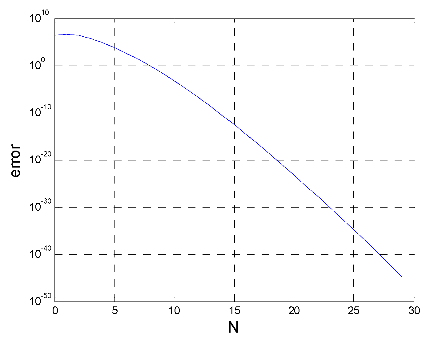
3.1. Convergence of the Approximate Analytical MTF Expression

To achieve Equation (14), in practice, the infinitely many terms involving the Bessel function of the first kind in Equation (14) needs to be approximated to the sum of the finite terms, which brings the truncation error. The MTF can be calculated by truncating up to the 20th order Bessel functions of the first kind. The truncation error can be described as follows:

$$\begin{array}{l}\mathrm{E}\left(\mathrm{N}\right)=\sqrt{{\left[\frac{{\mathrm{J}}_0\left(2\mathsf{\pi }\mathrm{fD}\right)\sin \left(2\mathsf{\pi }\mathrm{fv}{\mathrm{t}}_{\mathrm{e}}\right)}{2\mathsf{\pi }\mathrm{fv}{\mathrm{t}}_{\mathrm{e}}}+\mathrm{A}+\mathrm{B}\right]}^2+{\left[\frac{{\mathrm{J}}_0\left(2\mathsf{\pi }\mathrm{fD}\right)\mathrm{si}{\mathrm{n}}^2\left(\mathsf{\pi }\mathrm{fv}{\mathrm{t}}_{\mathrm{e}}\right)}{\mathsf{\pi }\mathrm{fv}{\mathrm{t}}_{\mathrm{e}}}+\mathrm{C}-\mathrm{D}\right]}^2}\\ -\sqrt{{\left[\frac{{\mathrm{J}}_0\left(2\mathsf{\pi }\mathrm{fD}\right)\sin \left(2\mathsf{\pi }\mathrm{fv}{\mathrm{t}}_{\mathrm{e}}\right)}{2\mathsf{\pi }\mathrm{fv}{\mathrm{t}}_{\mathrm{e}}}+{\mathrm{A}}_{\mathrm{N}}+{\mathrm{B}}_{\mathrm{N}}\right]}^2+{\left[\frac{{\mathrm{J}}_0\left(2\mathsf{\pi }\mathrm{fD}\right)\mathrm{si}{\mathrm{n}}^2\left(\mathsf{\pi }\mathrm{fv}{\mathrm{t}}_{\mathrm{e}}\right)}{\mathsf{\pi }\mathrm{fv}{\mathrm{t}}_{\mathrm{e}}}+{\mathrm{C}}_{\mathrm{N}}-{\mathrm{D}}_{\mathrm{N}}\right]}^2}\end{array},$$

(15)

where ${\mathrm{A}}_{\mathrm{N}},{\mathrm{B}}_{\mathrm{N}},{\mathrm{C}}_{\mathrm{N}},{\mathrm{D}}_{\mathrm{N}}$ represent the finite N terms of $\mathrm{A},\mathrm{B},\mathrm{C},\mathrm{D}$, respectively. As the value of MTF is always greater than 0, the approximation error can be expressed as follows:

$$\mathrm{E}\left(\mathrm{N}\right)<\sqrt{\begin{array}{l}|{\left(\frac{{\mathrm{J}}_0\left(2\mathsf{\pi }\mathrm{fD}\right)\sin \left(2\mathsf{\pi }\mathrm{fv}{\mathrm{t}}_{\mathrm{e}}\right)}{2\mathsf{\pi }\mathrm{fv}{\mathrm{t}}_{\mathrm{e}}}+\mathrm{A}+\mathrm{B}\right)}^2+{\left(\frac{{\mathrm{J}}_0\left(2\mathsf{\pi }\mathrm{fD}\right)\mathrm{si}{\mathrm{n}}^2\left(\mathsf{\pi }\mathrm{fv}{\mathrm{t}}_{\mathrm{e}}\right)}{\mathsf{\pi }\mathrm{fv}{\mathrm{t}}_{\mathrm{e}}}+\mathrm{C}-\mathrm{D}\right)}^2\\ -{\left(\frac{{\mathrm{J}}_0\left(2\mathsf{\pi }\mathrm{fD}\right)\sin \left(2\mathsf{\pi }\mathrm{fv}{\mathrm{t}}_{\mathrm{e}}\right)}{2\mathsf{\pi }\mathrm{fv}{\mathrm{t}}_{\mathrm{e}}}+{\mathrm{A}}_{\mathrm{N}}+{\mathrm{B}}_{\mathrm{N}}\right)}^2-{\left(\frac{{\mathrm{J}}_0\left(2\mathsf{\pi }\mathrm{fD}\right)\mathrm{si}{\mathrm{n}}^2\left(\mathsf{\pi }\mathrm{fv}{\mathrm{t}}_{\mathrm{e}}\right)}{\mathsf{\pi }\mathrm{fv}{\mathrm{t}}_{\mathrm{e}}}+{\mathrm{C}}_{\mathrm{N}}-{\mathrm{D}}_{\mathrm{N}}\right)}^2|\end{array}}.$$

(16)

To simplify Equation (16), the truncation error can be expressed by the infinitely many terms involving the Bessel function after 2Nth order, as follows:

$$\mathsf{\Delta }\mathrm{M}=\mathrm{M}-{\mathrm{M}}_{\mathrm{N}}\left(\mathrm{M}=\mathrm{A},\mathrm{B},\mathrm{C},\mathrm{D}\right).$$

(17)

As the MTF of the image motion is always less than 1, Equation (16) can be presented as follows:

$$\begin{array}{ll}\mathrm{E}\left(\mathrm{N}\right)& <\sqrt{\left(2\mathsf{\Delta }\mathrm{A}+2\mathsf{\Delta }\mathrm{B}+2\mathsf{\Delta }\mathrm{C}+2\mathsf{\Delta }\mathrm{D}\right)}\\ & <2\left(\left|\mathsf{\Delta }\mathrm{A}\right|+\left|\mathsf{\Delta }\mathrm{B}\right|+\left|\mathsf{\Delta }\mathrm{C}\right|+\left|\mathsf{\Delta }\mathrm{D}\right|\right)\end{array}.$$

(18)

Substituting in Equation (17), Equation (18) can be written as follows:

$$\begin{array}{ll}\mathrm{E}\left(\mathrm{N}\right)& <2{\displaystyle \sum _{\mathrm{n}=2\mathrm{N}+1}^{\infty }\left|{\mathrm{J}}_{\mathrm{n}}\left(2\mathsf{\pi }\mathrm{fD}\right)\left[\frac{\sin (\mathrm{n}\mathsf{\omega }+2\mathsf{\pi }\mathrm{fv}){\mathrm{t}}_{\mathrm{e}}}{\mathrm{n}\mathsf{\omega }+2\mathsf{\pi }\mathrm{fv}}+\frac{\sin (\mathrm{n}\mathsf{\omega }-2\mathsf{\pi }\mathrm{fv}){\mathrm{t}}_{\mathrm{e}}}{\mathrm{n}\mathsf{\omega }-2\mathsf{\pi }\mathrm{fv}}\right]\right|}\\ & +2{\displaystyle \sum _{\mathrm{n}=2\mathrm{N}+1}^{\infty }\left|{\mathrm{J}}_{\mathrm{n}}\left(2\mathsf{\pi }\mathrm{fD}\right)\left[\frac{1-\cos (\mathrm{n}\mathsf{\omega }+2\mathsf{\pi }\mathrm{fv}){\mathrm{t}}_{\mathrm{e}}}{\mathrm{n}\mathsf{\omega }+2\mathsf{\pi }\mathrm{fv}}-\frac{1-\cos (\mathrm{n}\mathsf{\omega }-2\mathsf{\pi }\mathrm{fv}){\mathrm{t}}_{\mathrm{e}}}{\mathrm{n}\mathsf{\omega }-2\mathsf{\pi }\mathrm{fv}}\right]\right|}\end{array}.$$

(19)

Based on the properties of the trigonometric functions and the range of parameters of the image motion, the approximation error is given as follows:

$$\mathrm{E}\left(\mathrm{N}\right)<8{\displaystyle \sum _{\mathrm{n}=2\mathrm{N}+1}^{\infty }\left|{\mathrm{J}}_{\mathrm{n}}\left(2\mathsf{\pi }\mathrm{fD}\right)\right|}.$$

(20)

The integral order Bessel function of the first kind can be expressed in the form of a power series, as follows:

$${\mathrm{J}}_{\mathrm{n}}\left(\mathrm{x}\right)={\displaystyle \sum _{\mathrm{m}=0}^{\infty }{\left(-1\right)}^{\mathrm{m}}\frac{1}{\mathsf{\Gamma }\left(\mathrm{m}+1\right)\mathsf{\Gamma }\left(\mathrm{m}+\mathrm{n}+1\right)}}{\left(\frac{\mathrm{x}}{2}\right)}^{2\mathrm{m}+\mathrm{n}}.$$

(21)

Substituting Equation (21) into Equation (20), the truncation error can be expressed as follows:

$$\mathrm{E}\left(\mathrm{N}\right)<8{\displaystyle \sum _{\mathrm{n}=2\mathrm{N}+1}^{\infty }\left|{\displaystyle \sum _{\mathrm{m}=0}^{\infty }{\left(-1\right)}^{\mathrm{m}}\frac{1}{\mathrm{m}!\left(\mathrm{m}+\mathrm{n}\right)!}}{\left(\mathsf{\pi }\mathrm{fD}\right)}^{2\mathrm{m}+\mathrm{n}}\right|}<8{\displaystyle \sum _{\mathrm{n}=2\mathrm{N}+1}^{\infty }\left|{\displaystyle \sum _{\mathrm{m}=0}^{\infty }{\left(-1\right)}^{\mathrm{m}}\frac{1}{\mathrm{m}!\mathrm{n}!}}{\left(\mathsf{\pi }\mathrm{fD}\right)}^{2\mathrm{m}+\mathrm{n}}\right|}.$$

(22)

According to the Maclaurin’s series of ${\mathrm{e}}^{\mathrm{x}}$, which is presented as the following:

$${\mathrm{e}}^{\mathrm{x}}={\displaystyle \sum _{\mathrm{k}=0}^{2\mathrm{N}}\frac{{\mathrm{x}}^{\mathrm{k}}}{\mathrm{k}!}}+\frac{{\mathrm{e}}^{\mathsf{\xi }}}{(2\mathrm{N}+1)!}{\mathrm{x}}^{2\mathrm{N}+1},\mathsf{\xi }\in \left(0,\mathrm{x}\right),$$

(23)

the upper bound to the absolute error is expressed as follows:

$$\mathrm{E}\left(\mathrm{N}\right)<8\left|{\displaystyle \sum _{\mathrm{n}=2\mathrm{N}+1}^{\infty }\frac{1}{\mathrm{n}!}{\left(\mathsf{\pi }\mathrm{fD}\right)}^{\mathrm{n}}{\displaystyle \sum _{\mathrm{m}=0}^{\infty }\frac{1}{\mathrm{m}!}}{\left(\mathsf{\pi }\mathrm{fD}\right)}^{2\mathrm{m}}}\right|<\left|\frac{8\exp \left[{\left(\mathsf{\pi }\mathrm{fD}\right)}^2+\left(\mathsf{\pi }\mathrm{fD}\right)\right]}{(2\mathrm{N}+1)!}{\left(\mathsf{\pi }\mathrm{fD}\right)}^{2\mathrm{N}+1}\right|.$$

(24)

With Equation (24), the upper bound error can be calculated. However, it is necessary to emphasize that fewer order Bessel functions are required generally. A plot of the upper limit error for 2Nth order approximation at the spatial frequency $\mathrm{f}=1/\mathrm{D}$ is shown in Figure 1. As can be seen, up to the 20th order Bessel functions are needed for an approximation error less than $10^{-20}$. In this paper, up to 20th order Bessel functions are used to calculate the MTF for the image motion.

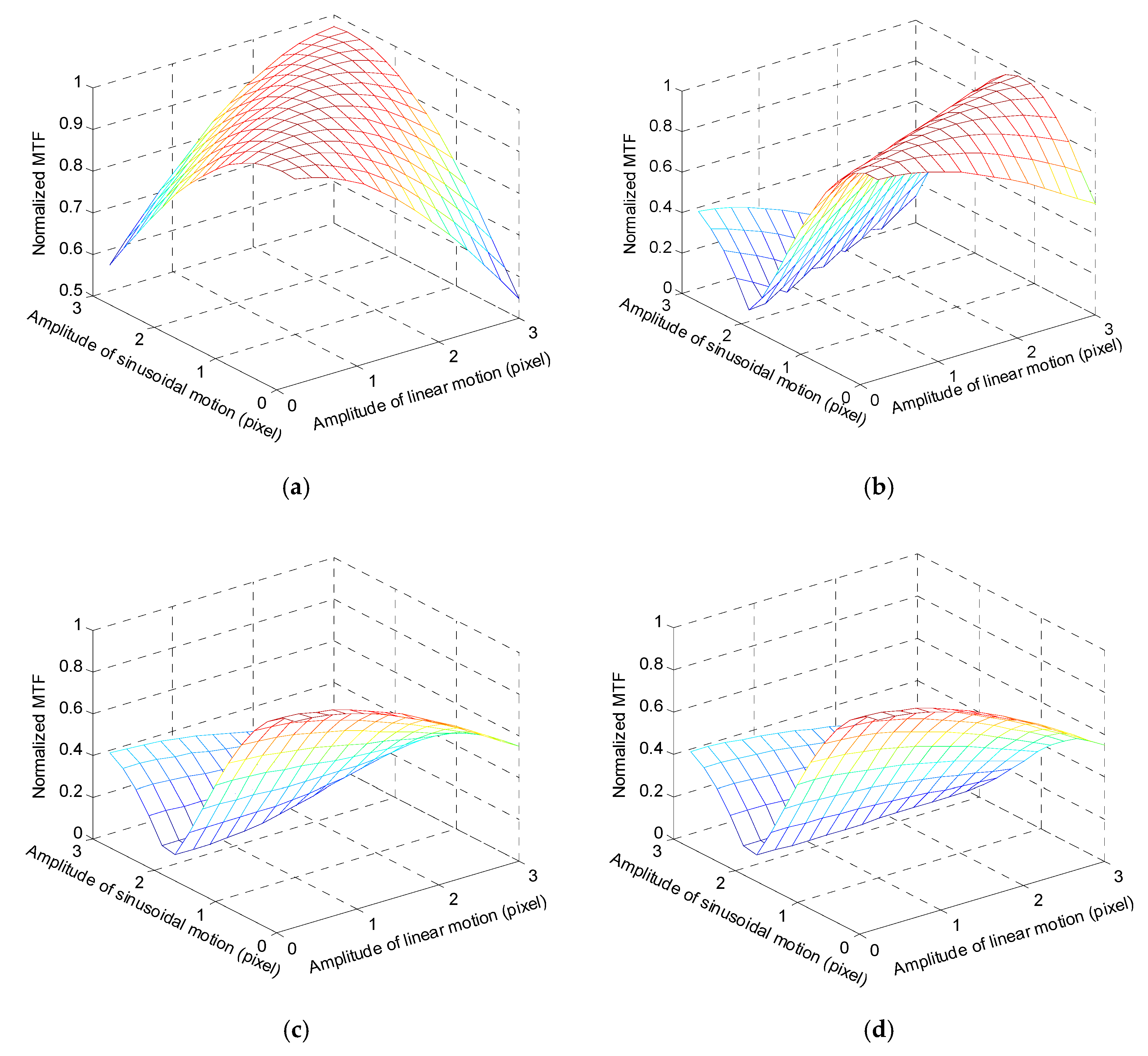
3.2. Expression Analysis of MTF for Image Motion

According to the early research on MTF for sinusoidal motion, sinusoid oscillations are often classified as low frequency, $\frac{{\mathrm{t}}_{\mathrm{e}}}{\mathrm{T}}<1$, and high frequency, $\frac{{\mathrm{t}}_{\mathrm{e}}}{\mathrm{T}}>1$, based on the ratio of the exposure period to the vibration period [20], where ${\mathrm{t}}_{\mathrm{e}}$ represents the exposure time and $\mathrm{T}$ is the period of sinusoidal vibration.

In this section, we used Equation (14) to calculate the MTF for sinusoidal motion with different ratios. Figure 2 shows the simulation results. As can be seen from the displayed results, the higher the ratio is, the faster the MTF declines, which means that a high-frequency vibration can cause much larger and more serious image blurring when the blur radius is certain and the linear motion is fixed.

In accordance with the calculation formula, the MTF for complex motions depends on the blur radius of linear motion and the amplitude of the sinusoidal vibration. Figure 3 shows the relationship between the MTF at the Nyquist frequency and the amplitudes of the motions, where Figure 3a–d represent the sinusoidal motion with different ratios of $\frac{{\mathrm{t}}_{\mathrm{e}}}{\mathrm{T}}$.

It can be seen from Figure 3 that the MTF decreases rapidly for a high ratio of sinusoidal motion. Figure 3a shows that 1/4 of the cycle of low-frequency sinusoidal vibration in the exposure time can be approximated to linear motion, which is proven by the literature [17]. Figure 3c,d show similar curves, indicating that sinusoidal vibrations with different frequencies and certain amplitudes have an equal effect on MTF, when the ratio of $\frac{{\mathrm{t}}_{\mathrm{e}}}{\mathrm{T}}$ is an integer. This conclusion is consistent with the results obtained from the MTF for only sinusoidal image motion. However, it can be seen in Figure 2 that the MTFs for high-frequency sinusoidal motions with an integer ratio are the same only in some certain spatial frequencies. When the frequency of the sinusoidal vibration increases, the MTF curve tends to be a certain curve.

4. Simulation Experiment

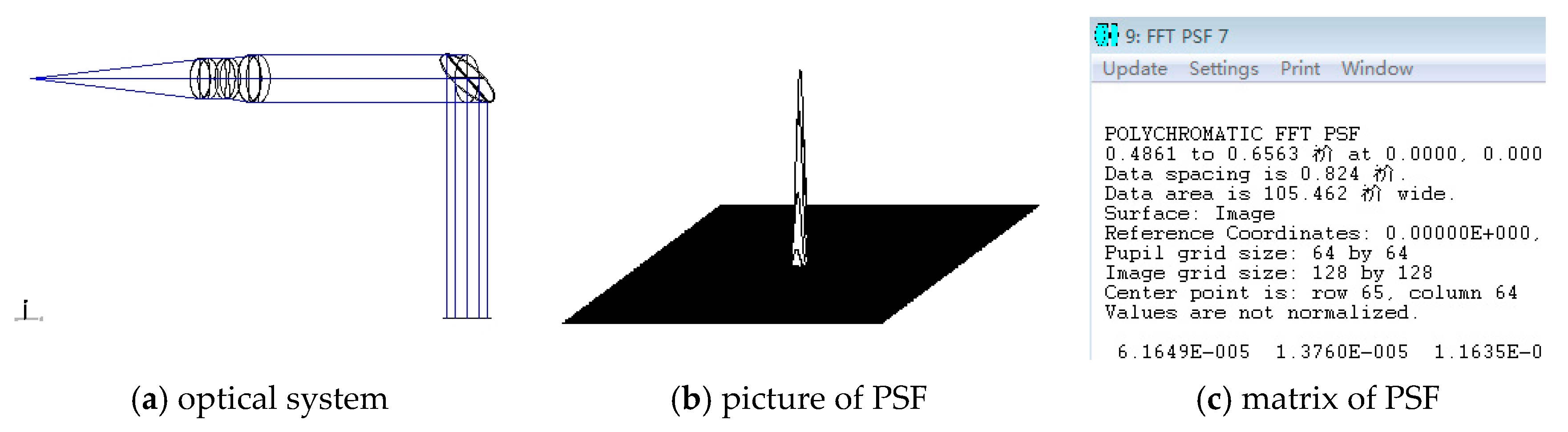
4.1. Simulation Method

To verify the validity of the MTF calculation method, a fast-steering mirror (FSM) and vibration platforms are usually required to give rise to sinusoidal vibration and linear image motion. In this paper, we used a mixed signal of sinusoidal and linear motion to actuate the FSM, which generated a complex motion at the focal plane in one direction. Figure 4 shows the experimental optical system [21,22]. However, the results may be inaccurate because of the pointing error of FSM and the aberrations of the optical system, when the motions are complicated.

Considering the actual working process of the FSM in an optical system, we proposed a simulation method to calculate the MTF in an optical system affected by vibration. In the simulation experiments, all of the data and simulation images were obtained from ZEMAX (2009, ZEMAX Development Corporation, USA and 2009) and MATLAB(R2012b, MathWorks, USA and 2012) [23,24]. We designed a simple optical system based on Figure 4 using ZEMAX as shown in Figure 5a. It was made of two groups of system: FSM and convergent lens. The point spread function (PSF) of the system and its data are seen in Figure 5b,c. According to the PSF acquired in ZEMAX, the actual process of the real system can be simulated by a simulation method programmed by MATLAB. The simulation method used ZEMAX to get the PSF of the optical system, and used MATLAB to simulate the effects of the image motions on the PSF. In that case, the MTF of the optical system affected by the image motion can be calculated by the PSF. The method simulates the influence of image motion on the MTF of the optical system in a period of time. The intuitive explanation for this method is as follows. Ideally, the reciprocating motion of the FSM causes the system PSF response to move spatially, without affecting the distribution of the intensity. These displacements are integrated during the exposure. The PSF for the image motion is obtained by adding up and normalizing the PSFs of the optical system with multiple instantaneous moments, which are sampled in a single exposure time by changing the position of the intensity matrix based on MATLAB. Thus, the MTF for the image motion can be calculated by Equation (25).

$$\mathrm{MTF}={\displaystyle \underset{-\infty }{\overset{\infty }{\int }}\mathrm{PSFexp}(-\mathrm{i}2\mathsf{\pi }\mathrm{fx})\mathrm{dx}}$$

(25)

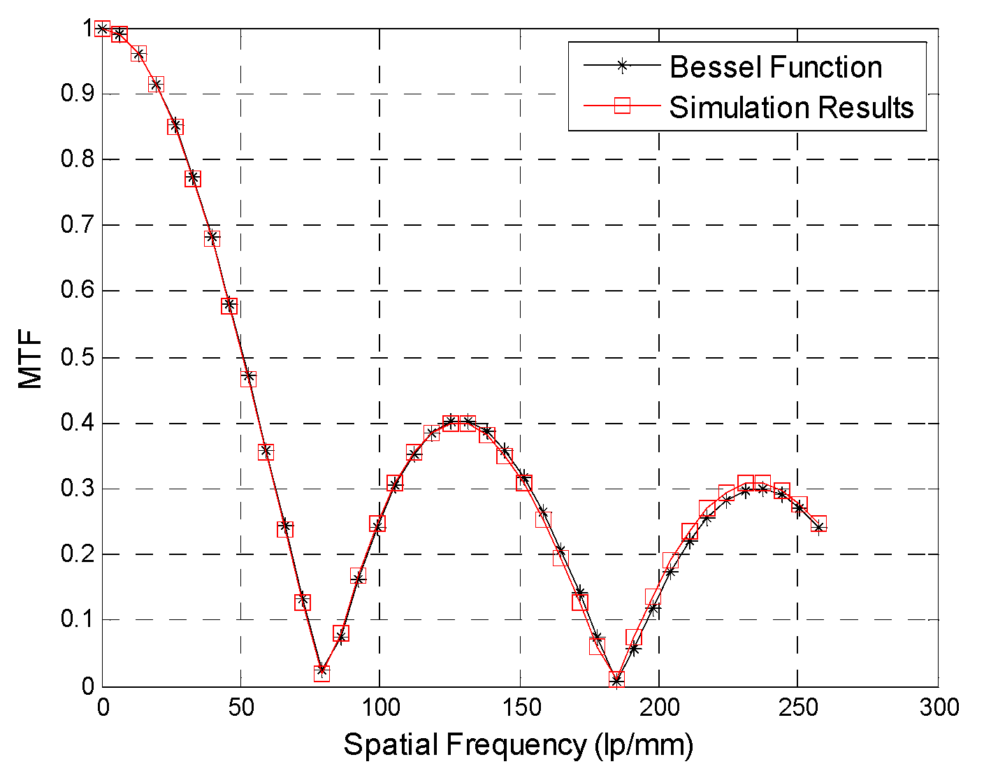
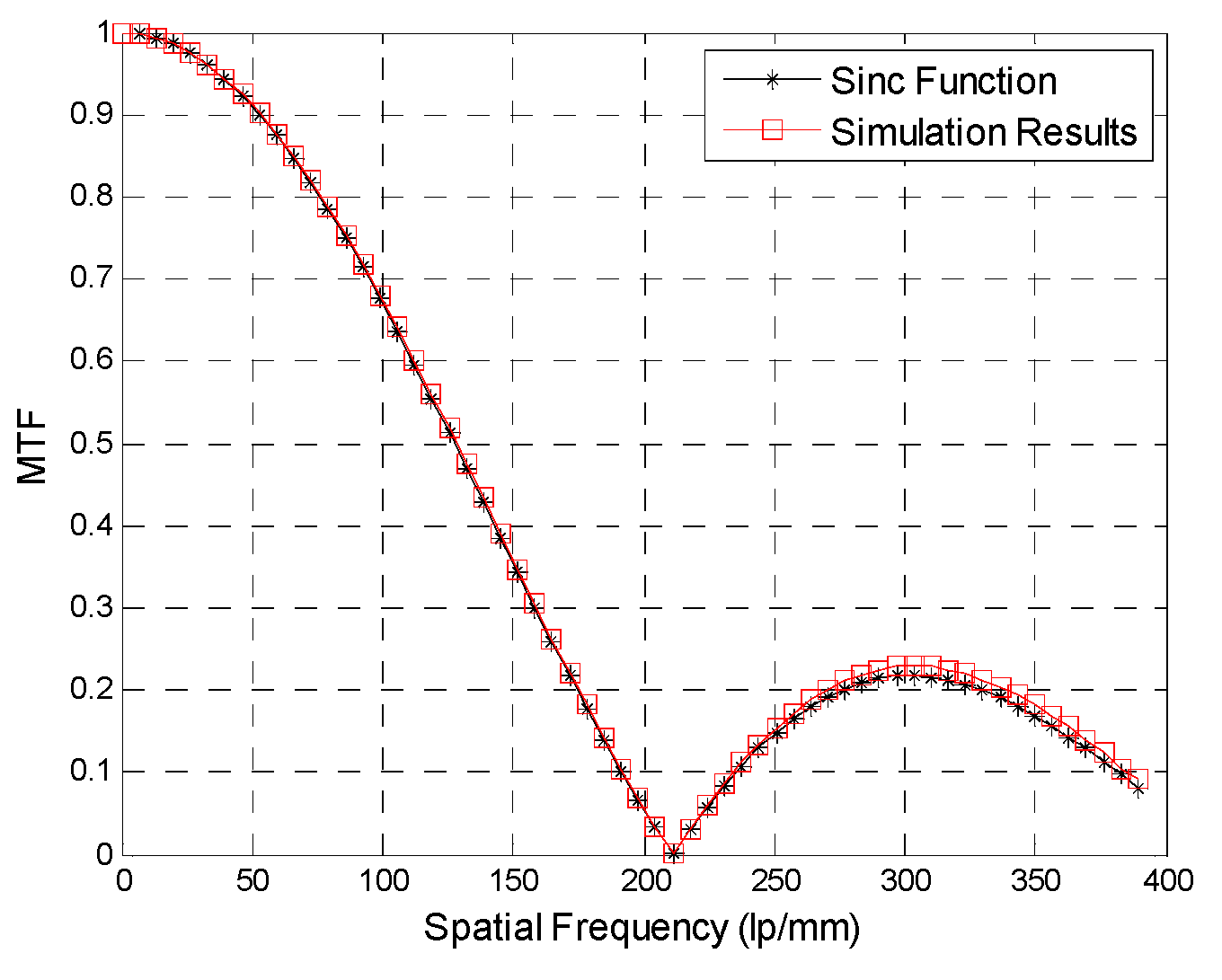
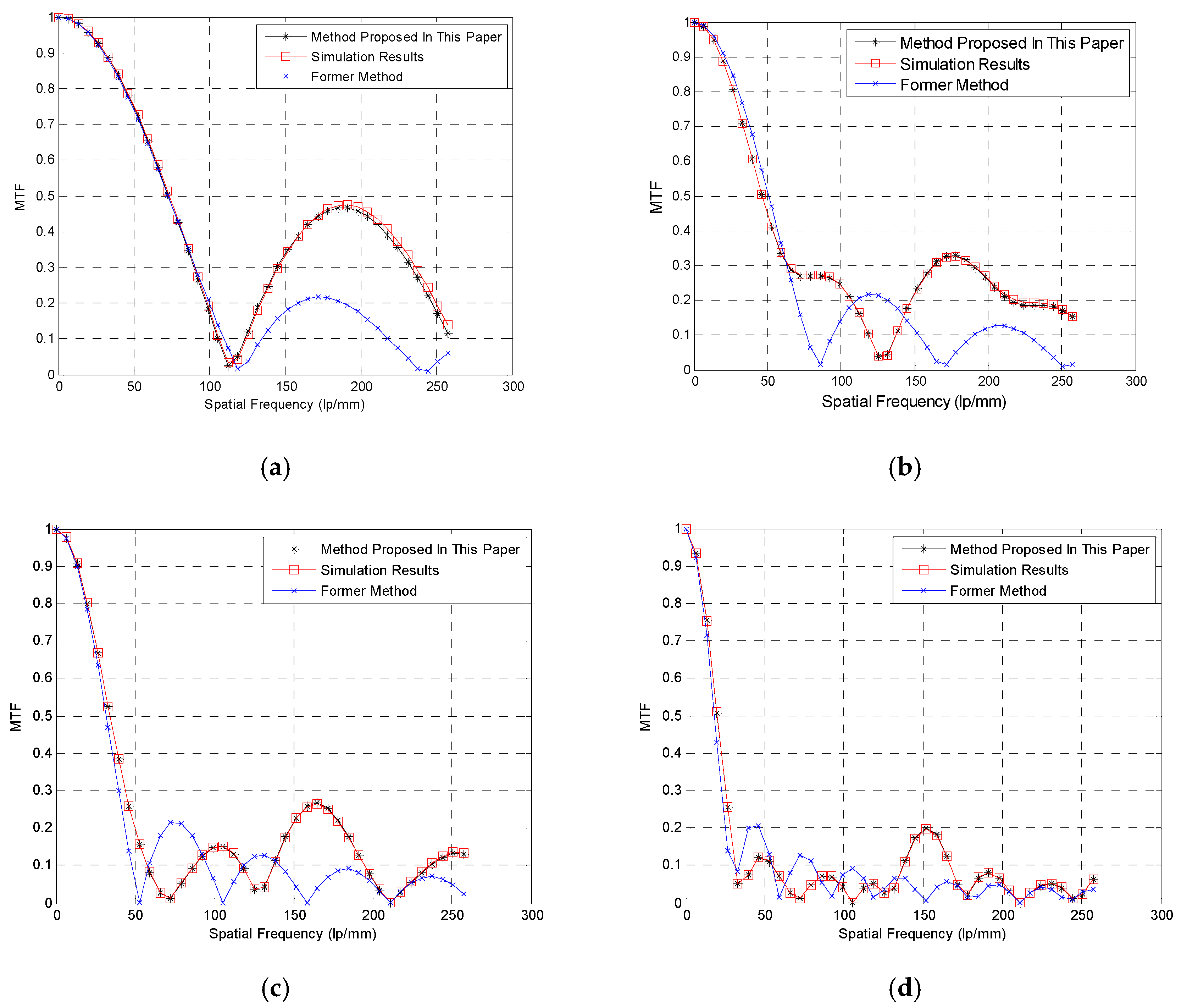
4.2. Simulation Results

As mentioned above, the simulation method is available for calculating the MTF for arbitrary image motions, which is illustrated theoretically. Therefore, the simulation method works in the case of a simple form of image motion, such as linear motion and sinusoidal motion. The simulation method can be verified in the case of simple form of image motion, such as linear motion and sinusoidal motion. For the data shown in Figure 5b, the image plane is $76\mathsf{\mu }\mathrm{m}\times 76\mathsf{\mu }\mathrm{m}$, with 128 × 128 sampling grids and 256 × 256 displaying grids. The maximum sampling frequency is 16.89 lp/mm.

Firstly, the simulation method is applied to the linear image motion. According to the Nyquist sampling theorem, linear motion can be sampled twice in the exposure. The MTF for the linear motion derived by other literature can be expressed as follows [11]:

$$\mathrm{MTF}\left(\mathrm{f}\right)=\frac{\sin \left(2\mathsf{\pi }\mathrm{fv}{\mathrm{t}}_{\mathrm{e}}\right)}{2\mathsf{\pi }\mathrm{fv}{\mathrm{t}}_{\mathrm{e}}}=\sin \mathrm{c}\left(2\mathsf{\pi }\mathrm{fd}\right),$$

(26)

where $\mathrm{d}$ is the non-circular blur radius of the linear motion. Figure 6 shows the MTFs calculated by the sinc function and the MTFs calculated by the simulation method.

To evaluate the simulation results, the average relative error is proposed as in Equation (27).

$$\mathrm{erro}{\mathrm{r}}_{\mathrm{relative}}=\frac{1}{\mathrm{k}}{\displaystyle \sum _{\mathrm{n}=1}^{\mathrm{k}}\left|\frac{\mathrm{MT}{\mathrm{F}}_{\mathrm{n}}-\mathrm{MT}{\mathrm{F}}_{\mathrm{n}}^{\prime }}{\mathrm{MT}{\mathrm{F}}_{\mathrm{n}}^{\prime }}\right|}\times 100\%,$$

(27)

where $\mathrm{MT}{\mathrm{F}}_{\mathrm{n}}$ represents the simulated result, $\mathrm{MT}{\mathrm{F}}_{\mathrm{n}}^{\prime }$ is the theoretical result and $\mathrm{k}$ stands for the quantity of the frequency points in the simulation. The average relative error for the linear motion calculated by Equation (27) is 3.23%.

According to the existing research, the MTF for sinusoidal motion is presented in the form of the Bessel function of the first kind. The expression can be described as follows [12]:

$$\mathrm{MTF}={\mathrm{J}}_0\left(2\mathsf{\pi }\mathrm{fD}\right),$$

(28)

where $\mathrm{D}$ stands for the amplitude of the sinusoidal motion. The Nyquist sampling theorem indicates that the sinusoidal signal needs to be sampled at least twice in a cycle. However, studies show that sampling twice in a cycle is not capable of restoring the original sinusoidal signal. In this case, we simulated the sinusoidal vibration signal by sampling 12 times in one period. The comparisons between the simulation results and the theoretical results are presented in Figure 7. The average relative error for the sinusoidal motion is 5.14%.

We used the simulation method to calculate the MTF for the mixed image motion of linear motion and sinusoidal motion. The PSF for the complex motion acquired by ZEMAX and MATLAB is shown in Figure 8.

As mentioned above in Section 1, the former method used the MTF calculation formula for linear motion to calculate the MTF for the complex image motion in the case of short exposure time [17]. The calculation formula is expressed as Equation (26). In order to compare the calculation method presented in this paper with the former method, the simulation experiments were carried out with different exposure times. In the simulation experiment, the velocity of the linear motion was 12 pixels per second, and the amplitude of sinusoidal vibration was eight pixels. The frequency of sinusoidal vibration was set as 1 Hz, and the exposure time range was from 0.5 s to 4 s. The curves of the MTF calculated by the simulation method and the calculation method in different exposure times are presented in Figure 9. Figure 9 also shows the calculated MTFs by the former methods using Equation (26). The average relative errors and the running time of the two methods are compared in

Table 1. The average relative errors and running time of the two methods.

Exposure Time (s)	Our Method		Former Method
	Errors	Running Time (s)	Errors	Running Time (s)
0.5	4.57%	1.452	39.71%	0.752
1	1.37%	1.448	65.29%	0.749
2	1.91%	1.415	106.6%	0.751
4	4.59%	1.425	891.86%	0.747

. As can be seen in Table 1, with different exposure times, the average relative error between the MTFs calculated by the method proposed in this paper and the simulation method are 4.57%, 1.37%, 1.91% and 4.59%, separately. The average relative errors between the MTFs calculated by the former method and the simulation method are 39.71%, 65.29%, 106.6%, and 891.86%, separately. Table 1 also shows the running time of the two methods.

As can be seen in Figure 9, the trend of MTF calculated by the proposed method varies with the exposure time, caused by the change of the blur radius of the linear motion and the frequency of the sinusoidal vibration. We can see from Table 1 that the errors between the MTF calculated by Equation (26) and the simulation results increase with the increase of exposure time. We can conclude that, despite the increase in running time, the MTFs calculated by our method, resulting in a less than 5% average relative error, are more similar to the simulation results than the former method.

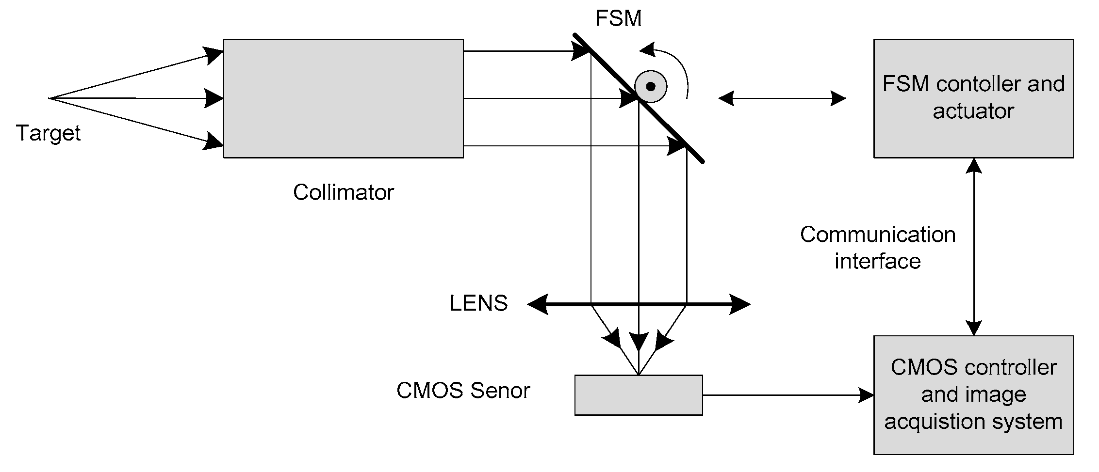
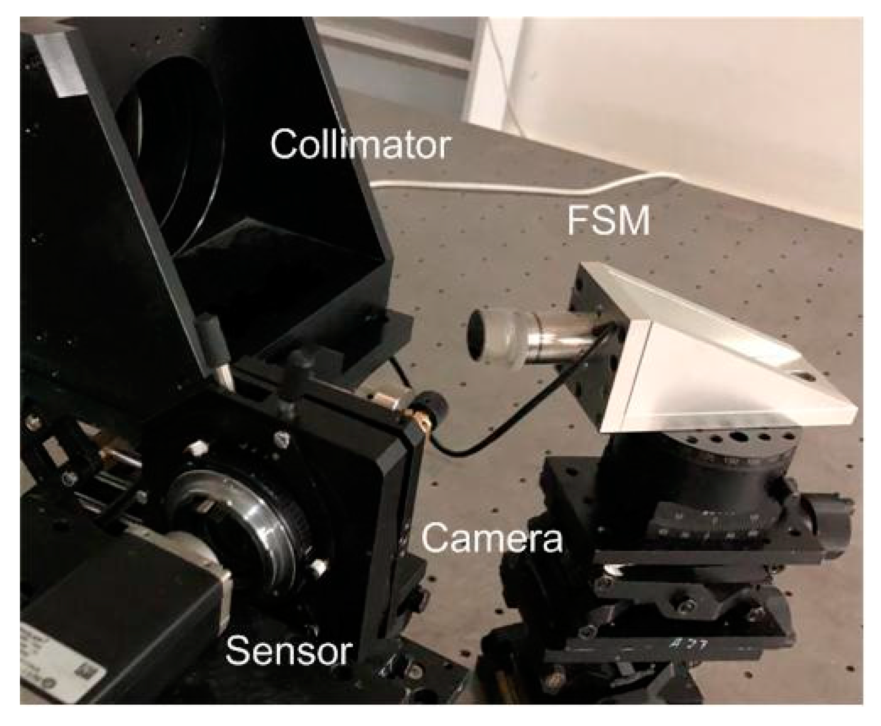
5. Laboratory Experiments for Validation

To further verify the theoretical analysis, we performed an experiment using the experimental setup in Figure 4. In these experiments, the Basler camera (Basler, Germany) piA2400-17gm, which has a pixel size of $3.45\times 3.45\mathsf{\mu }\mathrm{m}$, and an image size of 2456 × 2058 pixels, was used. The FSM that we used was S-330.2SL (Power integrations, USA) produced by the Pi company. The closed-loop tilt angle provided by the FSM is 2 mrad. Figure 10 shows the actual experiment setup. The image blurred by the complex motion is presented in Figure 11. The blur radius of linear motion was 12 pixels, and the amplitude of the sinusoidal motion was eight pixels. The exposure time was 1 s. The frequency range of the sinusoidal vibration generated by the FSM was from 0.5 to 4 Hz. Figure 12 shows the MTF for the complex motion measured by the point-source method [25], when the frequencies of the sinusoidal motions are different. Compared with Figure 2, the MTFs in Figure 12 have the same tendency. The MTFs measured from the images, and the MTFs calculated by our method are basically consistent, as shown in Figure 13. The average relative error calculated by Equation (27) is presented in

Table 2. The average relative errors between the theoretical results and experimental results.

The Frequency of Sinusoidal Vibration (Hz)	The Average Relative Error
0.5	7.21%
1	9.44%
2	11.38%
4	10.89%

.

6. Conclusions

The MTF of images is a significant index to evaluate the performance of remote-sensing cameras. However, calculating the MTF for image motion is usually difficult when the form of the image motion is complicated. In this paper, we propose a new approach to calculate the MTF for the mixed image motion of multiple forms of motion. By replacing the integral of the trigonometric functions with the summation of infinitely many terms involving the Bessel function, dynamic MTFs for the complex motion of linear motion and sinusoidal motion is expressed as an infinite sum of the integral order Bessel functions of the first kind. In order to obtain the numerical results of the MTF, the truncation error obtained by the use of finite order sum approximations instead of infinite sums is calculated, which gives satisfactory results. The MTF calculated model indicates that, with the same blur radius, the image degradation due to high-frequency vibration is more severe than that for low-frequency vibration. To verify the validity of the MTF calculation formula, a simulation method is proposed to calculate the MTF for the image motion. The results of the simulation experiment show that the mean value of the difference between the calculation model and the simulation method is less than 5%. Furthermore, laboratory experiments were carried out, and the average relative error was less than 12%. Hence, the proposed method improves the calculation accuracy and the applicability of the MTF calculation method for complex motion. This study will be of great significance for indicator design and image restoration of remote-sensing imaging.

References

1. Jun, P.; Chengbang, C.; Ying, Z.; Mi, W. Satellite Jitter Estimation and Validation Using Parallax Images. Sensors 2017, 17, 83. [Google Scholar]
2. Jin, L.; Fei, X.; Ting, S.; Zheng, Y. Efficient assessment method of on-board modulation transfer function of optical remote sensing sensors. Opt. Express 2015, 23, 6187–6208. [Google Scholar]
3. Taiji, L.; Xucheng, X.; Junlin, L.; Chengshan, H.; Kehui, L. A high-dynamic-range optical sensing imaging method for digital TDI CMOS. Appl. Sci. 2017, 7, 1089. [Google Scholar]
4. Peng, X.; Qun, H.; Changning, H.; Yongtian, W. Degradation of modulation transfer function in push-broom camera caused by mechanical vibration. Opt. Laser Technol. 2003, 35, 547–552. [Google Scholar]
5. Wei, Z.; Hans, Z.; Andreas, S. Wafer-scale fabricated thermo-pneumatically tunable microlenses. Light Sci. Appl. 2014, 3. [Google Scholar] [CrossRef]
6. Moojoong, K.; Jaisuk, Y.; Dong-Kwon, K.; Hyunjung, K. Measurement of contrast and spatial resolution for the photothermal imaging method. Appl. Sci. 2019, 9, 1996. [Google Scholar]
7. JiaQi, W.; Changxiang, Y. Space optical remote sensor image motion velocity vector computational modeling, error budget and synthesis. Chin. Opt. Lett. 2005, 3, 414–417. [Google Scholar]
8. Mark, E.P.; William, G.M. Optical transfer functions, weighting functions, and metrics for images with two-dimensional line-of-sight motion. Opt. Eng. 2016, 55, 063108. [Google Scholar]
9. Chenghao, Z.; Zhile, W. Mid-frequency MTF compensation of optical sparse aperture system. Opt. Express 2018, 26, 6973–6992. [Google Scholar]
10. Jin, L.; Zilong, L. Using sub-resolution features for self-compensation of the modulation transfer function in remote sensing. Opt. Express 2017, 25, 4018–4037. [Google Scholar]
11. Hansung, K.; Heonyong, K.; Moo-Hyun, K. Real-time inverse estimation of ocean wave spectra from vessel-motion sensors using adaptive kalman filter. Appl. Sci. 2019, 9, 2797. [Google Scholar]
12. Hadar, O.; Dror, I.; Kopeika, N.S. Image resolution limits resulting from mechanical vibrations. Part IV: Real-time numerical calculation of optical transfer functions and experimental verification. Opt. Eng. 1994, 33, 566–578. [Google Scholar] [CrossRef]
13. Yanlu, D.; Yalin, D. Dynamic modulation transfer function analysis of images blurred by sinusoidal vibration. J. Opt. Soc. Korea 2016, 20, 762–769. [Google Scholar]
14. Jin, L.; Zilong, L.; Si, L. Suppressing the images smear of the vibration modulation transfer function for remote-sensing optical cameras. Appl. Opt. 2017, 56, 1616–1624. [Google Scholar]
15. Adrian, S.; Norman, S.K. Analytical method to calculate optical transfer functions for image motion and vibrations using moments. J. Opt. Soc. Korea 1997, 14, 388–396. [Google Scholar]
16. Liude, T.; Tao, W. Calculation of optical transfer function for image motion based on statistical moments. Acta Opt. Sin. 2017, 37. [Google Scholar] [CrossRef]
17. Rudoler, S.; Hadar, O.; Fisher, M.; Kopeika, N.S. Image resolution limits resulting from mechanical vibrations Part 2: Experiment. Opt. Eng. 1994, 305, 577–589. [Google Scholar]
18. Zhuxi, W.; Dunren, G. Introduction to Special Function; Peking University Press: Beijing, China, 2000; pp. 337–415. [Google Scholar]
19. Kun, G.; Lu, H.; Hongmiao, L.; Zeyang, D.; Guoqiang, N.; Yingjie, Z. Analysis of MTF in TDI-CCD subpixel dynamic super-resolution imaging by beam splitter. Appl. Sci. 2017, 7, 905. [Google Scholar]
20. Wenbao, G.; YaLin, D. Analysis of influence of vibration on transfer function in optics imaging system. Opt. Precis. Eng. 2009, 17, 314–320. [Google Scholar]
21. Yu, J.; Hua, F.; Jiang, W. Distortion evaluation method for the progressive addition lens–eye system. Opt. Commun. 2019, 445, 204–210. [Google Scholar] [CrossRef]
22. Xufen, X.; Hongda, F. Regularized slanted-edge method for measuring the modulation transfer function of imaging systems. Appl. Opt. 2018, 57, 6552–6558. [Google Scholar]
23. Chin-Ta, Y.; Jyun-Min, S. A study of optical design on 9 × zoom ratio by using a compensating liquid lens. Appl. Sci. 2015, 5, 608–621. [Google Scholar]
24. Xufen, X.; Yuncui, Z.; Hongyuan, W.; Wei, Z. Analysis and modeling of radiometric error caused by imaging blur in optical remote sensing systems. Infrared Phys. Technol. 2016, 77, 51–57. [Google Scholar]
25. Weiwei, X.; Liming, Z. On-orbit modulation transfer function detection of high resolution optical satellite sensor based on reflected point sources. Acta Opt. Sin. 2017, 37, 0728001-1-8. [Google Scholar] [CrossRef]
Figure 1. The upper bound error for the 2Nth order approximation at spatial frequency f = 1/D.
Applsci 09 05142 g001
Figure 2. Modulation transfer functions (MTFs) for sinusoidal motion with different frequency ratios when the linear motion is fixed.
Applsci 09 05142 g002
Figure 3. Comparison of the MTFs for different amplitudes of complex motions with different ratios, namely: (a) t e T = 0.25 ; (b) t e T = 0.5 ; (c) t e T = 1 ; (d) t e T = 2 .
Applsci 09 05142 g003
Figure 4. Sketch of the experimental setup. FSM: fast-steering mirror.
Applsci 09 05142 g004
Figure 5. Data acquired by ZEMAX. PSF: point spread function.
Applsci 09 05142 g005
Figure 6. The simulated MTF and theoretical MTF for linear motion.
Applsci 09 05142 g006
Figure 7. The simulated MTF and theoretical MTF for sinusoidal motion.
Applsci 09 05142 g007
Figure 8. The grayscale image of complex motion.
Applsci 09 05142 g008
Figure 9. MTFs in different exposure times, namely: (a) 0.5 s, (b) 1 s, (c) 2 s, and (d) 4 s.
Applsci 09 05142 g009
Figure 10. The experimental imaging system.
Applsci 09 05142 g010
Figure 11. The grayscale image acquired in the experiment.
Applsci 09 05142 g011
Figure 12. The MTFs with different frequencies, measured by the point-source method.
Applsci 09 05142 g012
Figure 13. The calculated MTF and the measured MTF for sinusoidal motion with different frequencies, namely: (a) 0.5 Hz, (b) 1 Hz, (c) 2 Hz, and (d) 4 Hz.
Applsci 09 05142 g013