Article

Synergetic Application of Multi-Criteria Decision-Making Models to Credit Granting Decision Problems

by
Vicente García
1,†,
J. Salvador Sánchez
2,*,† and
Ana I. Marqués
3,†
1
Department of Electrical and Computer Engineering, Universidad Autónoma de Ciudad Juárez, Ciudad Juárez 32310, Mexico
2
Institute of New Imaging Technologies, Department of Computer Languages and Systems, Universitat Jaume I, 12071 Castelló de la Plana, Spain
3
Department of Business Administration and Marketing, Universitat Jaume I, 12071 Castelló de la Plana, Spain
*
Author to whom correspondence should be addressed.
These authors contributed equally to this work.
Appl. Sci. 2019, 9(23), 5052; https://doi.org/10.3390/app9235052
Submission received: 5 November 2019 / Revised: 19 November 2019 / Accepted: 20 November 2019 / Published: 22 November 2019
(This article belongs to the Section Computing and Artificial Intelligence)

Abstract

:
Although various algorithms have widely been studied for bankruptcy and credit risk prediction, conclusions regarding the best performing method are divergent when using different performance assessment metrics. As a solution to this problem, the present paper suggests the employment of two well-known multiple-criteria decision-making (MCDM) techniques by integrating their preference scores, which can constitute a valuable tool for decision-makers and analysts to choose the prediction model(s) more properly. Thus, selection of the most suitable algorithm will be designed as an MCDM problem that consists of a finite number of performance metrics (criteria) and a finite number of classifiers (alternatives). An experimental study will be performed to provide a more comprehensive assessment regarding the behavior of ten classifiers over credit data evaluated with seven different measures, whereas the Technique for Order of Preference by Similarity to Ideal Solution (TOPSIS) and Preference Ranking Organization METHod for Enrichment of Evaluations (PROMETHEE) techniques will be applied to rank the classifiers. The results demonstrate that evaluating the performance with a unique measure may lead to wrong conclusions, while the MCDM methods may give rise to a more consistent analysis. Furthermore, the use of MCDM methods allows the analysts to weight the significance of each performance metric based on the intrinsic characteristics of a given credit granting decision problem.

1. Introduction

The 2007–2008 global financial crisis and the recommendations on banking regulations have attracted the growing interest of institutions in credit and operational risk management, which has become a key determinant of success because incorrect decisions may lead to heavy losses. One major difficulty for financial institutions relates to credit granting and, more specifically, how to discriminate between default and non-default applicants.
Conventional methods for credit risk management have usually been based on subjective decisions made by analysts, using past experiences and well-established guidelines, but the increasing needs of companies and the huge amounts of financial data now available have motivated the design and application of more formal and precise techniques to make credit granting decisions more efficiently. Thus, the use of statistical and operations research methods depicted a first step towards this objective [1,2,3]. However, some assumptions of the statistical models are often difficult to meet in practice, which makes these methods theoretically null and void for databases with a limited number of samples [4]. In more recent years, important efforts have been addressed to exploit a variety of artificial intelligence and machine learning techniques, ranging from biologically inspired algorithms [5,6,7,8] to ensembles of classifiers [9,10,11,12], cluster analysis [13,14,15,16], and support vector machines [17,18,19], to shape solutions for both bankruptcy and credit risk prediction. An interesting advantage of these methods over the statistical models is that those automatically derive information from the past observations available in a data set, without assuming any specific prior knowledge.
From a practical viewpoint, credit granting decision can be expressed in the form of a two-class prediction problem in which a new case has to be assigned to one of the predetermined classes according to a set of input or explanatory attributes. These attributes or variables gather a diversity of information that summarizes both socio-demographic features and financial status of the credit applicants, whereas the classifier gives an output based on their financial solvency. Generally, a credit risk prediction system attempts to assign a credit applicant to either non-defaulter or defaulter. Let us assume a set of n past observations S = { ( x 1 , y 1 ) , , ( x n , y n ) } , where each instance x i is described by D input attributes, x i 1 , x i 2 , x i D , and y i is the class (defaulter/non-defaulter), then the objective of a prediction model δ is to estimate the value y for a new sample x , that is, δ ( x ) = y .
A considerable number of papers whose purpose has been to conduct a comparison of credit risk prediction algorithms are available in the literature, but their conclusions are often contradictory because of the criteria used for the evaluation. For instance, Desai et al. [20] showed that linear models perform worse than artificial neural networks when using the proportion of defaulters correctly predicted, and logistic regression achieves the highest proportion of non-defaulters and defaulters correctly predicted. Bensic et al. [6] noticed that the probabilistic neural networks are superior to learning vector quantization, classification and regression tree (CART), logistic regression, multilayer perceptron, and radial basis function based on the prediction accuracy. Yobas et al. [21] concluded that linear discriminant analysis is superior to decision trees, genetic algorithms, and neural networks when using the percentage of applicants correctly classified. Wang [12] showed that bagging and stacking with a decision tree as base classifier were the best performing algorithms when using type-I error, type-II error, and overall accuracy. Baesens et al. [17] found that the neural networks are superior to other methods based on the area under the receiver operating characteristic curve (ROC) curve, while the support vector machines perform the best in terms of overall accuracy. Bhaduri [22] tested some artificial immune systems against well-known classifiers on accuracy for two benchmark credit scoring data sets. Antonakis and Sfakianakis [23] compared linear discriminant analysis, decision trees, k-nearest neighbors decision rule, multilayer perceptron, naïve Bayes classifier, and logistic regression, pointing out that the k-nearest neighbors model performed the best in terms of accuracy, and the multilayer perceptron achieved the highest rate based on the Gini coefficient.
The contradictory conclusions of those studies and some other similar works suggest that no classifier can be considered the best on any performance evaluation metric. However, model selection is a subject of great interest for credit risk management, which advises the need of using more influential techniques for assessing the performance of prediction methods. Taking the limitations of individual performance scores into account, this paper suggests the synergetic application of MCDM models to provide a more comprehensive evaluation of credit granting decision systems. Thus, the TOPSIS and PROMETHEE methods rank a set of prediction models using a single scalar score that will be derived from aggregating their preference rates, showing that this technique allows for more consistent conclusions regarding the effectiveness of credit risk prediction models than the use of individual performance measures.
Henceforward, the paper is organized as follows. Section 2 offers an overview of MCDM and describes the two methods used here. Section 3 presents the details of the experimental design, with the description of the databases and the performance measures. Section 4 discusses the results of the experiments conducted. Section 5 summarizes the main conclusions that can be drawn from the present work and outlines possible avenues of further research.

2. Multiple-Criteria Decision-Making

Over the past several years, MCDM models have acquired a great relevance because this paradigm presents a number of features that make it especially suitable for analyzing hard real-life problems. One of the fundamental features of the MCDM methodologies refers to the fact that most of them can cope with both quantitative and qualitative data, along with the subjective opinions and/or the preferences of experts [24]. From a theoretical viewpoint, MCDM is a powerful component of operations research that encompasses some analytical tools and techniques to appraise the strengths and weaknesses of a set of M competing alternatives A = { a 1 , a 2 , , a M } evaluated on a family of N (usually conflicting) criteria of different nature C = { c 1 , c 2 , , c N } , with the objective of making an accurate decision regarding the preference judgment of the decision-maker [25,26]. Thus, an MCDM problem can be generally represented by means of a ( M × N ) decision matrix as that shown in Table 1.
Choosing the best alternative requires combining partial evaluations of each alternative into an aggregated value by using an aggregation operator Ψ : A R that relates a global value Ψ ( a i ) to alternative a i . This aggregation operator depends on the preferences of the analyst, which can be expressed regarding the relevance of criteria through weights w = { w 1 , w 2 , , w N } [ 0 , 1 ] N . Thus, the aggregation operator can be defined as
Ψ ( a i ) = j = 1 N w j a i j ,
where a i j are the partial evaluations of the alternative a i .
MCDM methods can be categorized into two general groups [27]: the multi-objective decision-making approach assumes a theoretically infinite (or a very large) number of alternatives, whereas the multi-attribute decision-making requires the assessment of a finite number of alternatives, which corresponds to the most common situation in financial decision-making problems (e.g., credit approval applications).
A rather different taxonomy identifies four categories [28]: (i) multi-objective mathematical programming, (ii) multi-attribute utility/value theory, (iii) outranking relations, and (iv) preference disaggregation analysis. As already pointed out, the present work concentrates on the outranking relations approach because it is recognized as one of the most effective ways to face the complexity of business and financial decision-making problems. In addition, unlike other MCDM techniques, the outranking relations methods are able to deal with any kind of problematics.
Performance assessment of classification algorithms requires dealing with various complementary criteria of interest, typically weighting the gains of each criterion against the others. Taking this into account, choosing the best performing prediction model can be considered as a particular MCDM problem, where M represents the number of prediction models (alternatives) and N expresses the number of performance assessment measures (criteria). In the framework of credit risk analysis, the MCDM techniques ought to allow analysts and decision-makers to pick up the algorithm that yields a closely optimal compromise between the evaluation criteria.
Well-known examples of the numerous MCDM algorithms that have been presented in the literature are TOPSIS (Technique for Order of Preference by Similarity to Ideal Solution), which is a representative of the multi-attribute value theory, and PROMETHEE (Preference Ranking Organization METHod for Enrichment of Evaluations), which belongs to the outranking techniques. Apart from their conceptual and implementational simplicity, both of these methods present some interesting benefits over other models [29]; for instance, they provide a single result in the form of a scalar value that constitutes the logic of human decision.

2.1. The TOPSIS Method

The basis of TOPSIS is to rank the alternatives or to discover the best alternative by simultaneously minimizing the distance to the positive ideal solution and maximizing the distance from the negative ideal solution [30]. The positive ideal solution ( a + ) is shaped as a mixture of the best performance values of any alternative for each criterion, whilst the negative ideal solution ( a ) corresponds to the mixture of the worst performance values.
Afterwards, the procedure follows by computing the separations of each alternative a i from the positive and negative ideal solutions, d i + and d i , using the N-dimensional Euclidean distance. Finally, the relative proximity to the ideal solution is computed as R i = d i / ( d i + + d i ) . Note that R i [ 0 , 1 ] because d i + 0 and d i 0 . Then, the alternatives can be ranked using this index in decreasing order, without the need for criterion preferences to be independent [31].
Let us assume an MCDM problem with M alternatives and N criteria represented as a decision matrix (Table 1); then, the TOPSIS method can be defined following the steps of Algorithm 1. It is worth noting that the alternatives are completely ranked based on their global utilities and, on the other hand, the criterion preferences are not required to be independent [30].
Algorithm 1 TOPSIS
1:
Compute the normalized decision matrix, where the normalized value n i j of the original score z i j is computed as n i j = z i j i = 1 M z i j 2       i = 1 , , M       j = 1 , , N .
2:
Compute the weighted normalized values v i j = w j z i j , where w j denotes the weight of the criterion c j and j = 1 N w j = 1
3:
Compute the positive and negative ideal solutions a + = { v 1 + , , v N + } = { ( max j v i j | i I ) , ( min j v i j | i J ) } , a = { v 1 , , v N } = { ( min j v i j | i I ) , ( max j v i j | i J ) } , where I and J are associated with benefit and cost criteria, respectively
4:
Compute the separation of each alternative from the positive and negative ideal solutions d j + = j = 1 N ( v i j v j + ) 2 and d j = j = 1 N ( v i j v j ) 2 i = 1 , , M .
5:
Compute the relative proximity to the ideal solution. The relative closeness of the alternative a i with respect to a + is defined as R i + = d i d i + + d i i = 1 , , M
6:
Rank alternatives based on the decreasing order of R i +

2.2. The PROMETHEE Method

The PROMETHEE methodology [32] intends to select the best alternatives (PROMETHEE I) or to sort the alternatives based on their values over different criteria (PROMETHEE II). As an outranking relations technique, the PROMETHEE method quantifies a ranking through the pairwise comparisons (differences) of alternatives ( a i , a j ) to determine the preference index π ( a i , a j ) [ 0 , 1 ] , which reflects how a i is preferred to a j on criterion c k . The calculation of the preference index is based on the specification of the normalized weights w k and the preference functions P k ( a i , a j ) for each criterion c k . The idea of this index is similar to that of the global concordance index in the ELECTRE methodology: the higher the preference index is, the higher the strength of the preference for a i over a j .
On the other hand, the PROMETHEE methodology also makes use of the concepts of positive and negative preference flows [33]: the positive preference flow ϕ + ( a i ) evaluates how a given alternative a i outranks the remaining alternatives, and the negative preference flow ϕ ( a i ) measures how an alternative a i is outranked by all the other alternatives. Finally, the global net preference flow, which is calculated as ϕ ( a i ) = ϕ + ( a i ) ϕ ( a i ) , indicates how an alternative a i is outranking ( ϕ ( a i ) > 0 ) or outranked ( ϕ ( a i ) < 0 ) by all the other alternatives on all the evaluation criteria. As a result, the alternative a i with the maximum global net preference flow will be deemed to be the best.
The general PROMETHEE methodology can be easily implemented in the form of a stepwise procedure as defined in Algorithm 2.
Algorithm 2 PROMETHEE
1:
For each pair ( a i , a j ) of a finite set of alternatives A = { a 1 , a 2 , , a M } , compute aggregated preference indices π ( a i , a j ) = k = 1 N P k ( a i , a j ) w k and π ( a j , a i ) = k = 1 N P k ( a j , a i ) w k
2:
Compute the positive and negative preference flows ϕ + ( a i ) = 1 M 1 a A π ( a i , A ) and ϕ ( a i ) = 1 M 1 a A π ( A , a i )
3:
Compute the net preference flow for each alternative as ϕ ( a i ) = ϕ + ( a i ) ϕ ( a i )
The global net preference flow ϕ ( a i ) indicates how an alternative a i is outranking ( ϕ ( a i ) > 0 ) or outranked ( ϕ ( a i ) < 0 ) by all the remaining alternatives on all the evaluation criteria. As a result, the alternative a i with the maximum global net preference flow will be identified as the best one.

3. Experiments

A series of experiments were conducted to assess the performance of a pool of classifiers through the TOPSIS and PROMETHEE tools for some credit granting decision problems, with the purpose of demonstrating that the synergetic application of MCDM models makes better decisions than using a single measure to determine the best performing prediction algorithm. The TOPSIS and PROMETHEE techniques were run with the Sanna open source software [34], whereas the classifiers were tested in the WEKA environment [35] using their default parameters (see Table 2):
  • Artificial neural networks: Bayesian belief network (Bnet), multilayer perceptron (MLP), and radial basis function (RBF);
  • Statistical models: naïve Bayes classifier (NBC), logistic regression (logR), support vector machine (SVM) and nearest neighbor classifier (1NN);
  • Rule-based classifier: RIPPER;
  • Decision trees: C4.5 and random forest (randF).

3.1. Data Sets

Table 3 reports some characteristics of the six real-life credit data sets used for the experiments, including the number of input or explanatory variables, the total number of instances and the number of instances in each class, and the imbalance ratio (IR) calculated as the ratio of the number of instances in the minority class to the number of instances in the majority class.
The Australian and German databases were obtained from the UCI Machine Learning Database Repository (http://archive.ics.uci.edu/ml/). The Australian database contains 690 samples of credit card applicants, 307 of which were labeled as solvent and 383 as unable to pay their debts; each sample is described by 14 input variables. The German credit database represents a credit screening application, comprising cases on 24 explanatory variables for a total of 1000 applicants: 700 were considered as creditworthy and 300 were labeled as non-creditworthy.
The Iranian database is an adaptation of a customers’ data set of a small private bank [36]. It contains 950 observations tagged as non-defaulters and 50 as defaulters, where each sample is formed by 27 explanatory variables. The Polish database consists of financial information regarding 120 firms registered over a 2-year period [37], with a total of 112 bankrupt and 128 non-bankrupt accounts. The Thomas database [38] comprises the data of 1225 applicants for a credit product, each one being shaped by 12 input attributes. Finally, the SabiSPQ database consists of 944 instances and 16 explanatory variables that describe firms whose accounts are established in the Spanish Mercantile Registry [39]. This constitutes a fully balanced data set with 472 healthy companies and 472 companies that failed during the period 2000–2003.

3.2. Performance Assessment Measures

Standard performance assessment measures for credit risk prediction include accuracy, area under the ROC curve, Kolmogorov–Smirnov statistic, geometric mean of accuracies, root mean squared error, Gini coefficient, and F-measure [38,40,41], among many others. For a problem with two classes, as is the case of the data set used in our experiments, most of these measures are easily obtained from a ( 2 × 2 ) confusion matrix as that shown in Table 4, where each entry represents the amount of correct (true-positive, true-negative) or wrong (false-positive, false-negative) decisions (classifications or predictions).
Numerous prediction systems typically employ the accuracy (Acc) rate to assess the performance of the classifiers, thus describing the proportion of correct classifications on a given data set. Nevertheless, practical and theoretical evidences demonstrate that the accuracy can be heavily biased regarding imbalance in class distribution and proportions of correct and incorrect classifications. As financial data are commonly strongly skewed, the area under the ROC curve (AUC) has been proposed as a suitable measure without regard to class distribution or misclassification costs [17,42]. For all practical purposes, the AUC for a two-class problem can be calculated as the arithmetic average of sensitivity (or true-positive rate, TP-rate) and specificity (or true-negative rate, TN-rate) [43]:
A U C = s e n s i t i v i t y + s p e c i f i c i t y 2 ,
where the sensitivity is the proportion of non-defaulters correctly classified, and the specificity denotes the proportion of defaulters classified as defaulters.
Other powerful measures based on simple indices are the geometric mean of accuracies (G-mean) and the F-measure. The geometric mean attempts to maximize the accuracy on each individual class while keeping a small difference between sensitivity and specificity. This metric penalizes those classifiers that yield large differences between true-positive and true-negative rates. It is worth pointing out that the geometric mean is closely linked to the distance to perfect classification in the ROC space:
G - m e a n = s e n s i t i v i t y · s p e c i f i c i t y .
On the other hand, the F-measure is defined as follows:
F - m e a s u r e = 2 · s e n s i t i v i t y · p r e c i s i o n p r e c i s i o n + s e n s i t i v i t y ,
where p r e c i s i o n = T P / ( T P + F P ) .
Finally, the root mean squared error (RMSE) corresponds to a standard performance evaluation metric widely-used in a variety of classification problems. Let p 1 , p 2 , , p m and a 1 , a 2 , , a m be the predicted and actual outputs on the test samples, respectively. The root mean squared error allows for measuring the difference between the predicted outputs and the true labels, estimating the deviation of the prediction model from the target value [44]:
R M S E = 1 m i = 1 m ( p i a i ) 2 .

3.3. Experimental Protocol

As databases are small in size, the performance of the classifiers were evaluated with the 5-fold cross-validation method because this seems to be a trustworthy strategy. Each data set was randomly partitioned into five stratified subsets of equal size: for each round, four blocks were used for training a learning algorithm and the remaining one for testing purposes (see Figure 1). In addition, ten repetitions were run for each trial in order to achieve more stable and reliable outcomes. Finally, the prediction results of all classifiers on the seven criteria were averaged across the 50 runs and then analyzed with the TOPSIS and PROMETHEE methods.

4. Results

Table 5, Table 6, Table 7, Table 8, Table 9 and Table 10 provide the results of each classifier on the seven performance assessment criteria (accuracy, root mean squared error, true-positive and true-negative rates, AUC, geometric mean, and F-measure) for each database. On the other hand, Table 11 reports the mean value across all data sets generated by each prediction model on each metric, which is here used to illustrate the performance of that classifier. For each performance metric, the best performing algorithm has been highlighted in boldface.
As can be observed in Table 5, Table 6, Table 7, Table 8, Table 9 and Table 10, no algorithm achieved the best performance across all criteria. For instance, when analyzing the results over the Australian database, logistic regression, RIPPER, and random forest were the prediction methods with the highest accuracy rate and F-measure, whereas the naïve Bayes classifier was the best performing algorithm in terms of TN-rate. Even a more obvious example is for the results over the Thomas database: the Bayesian belief network, logistic regression, MLP, and SVM achieved the highest rates when using the accuracy, the naïve Bayes classifier was the model with the highest true-negative rate and geometric mean, and MLP and random forest were the best algorithms on the F-measure.
These results show that there was a significant discrepancy regarding the set of criteria. Consequently, different conclusions about the best performing method could be drawn based on the performance assessment metric used. These conflicting outcomes depict a realistic scenario in which a pool of analysts or decision-makers might make very different decisions depending on the criteria used to measure the performance of a credit granting decision system. In our opinion, this reflects an illustrative example of real-life applications where the MCDM techniques should be taken into consideration for making more consistent, trustworthy decisions.
The conflicting points related to the employment of single performance assessment criteria led to carry out some experiments with the MCDM methods included in this study. Taking into account that identifying relative weights of criterion importance is nontrivial, one can use either subjective weighting methods or objective weighting methods [45]. While the subjective methods determine weights solely according to the decision-maker’s judgments/preferences, the objective methods define weights by solving mathematical models automatically without any consideration of the decision maker’s preferences. In general, objective weighting is applied to situations where reliable subjective weights cannot be obtained [46].
In this work, the weights used by the TOPSIS and PROMETHEE methods were set in line with the relative relevance of the performance evaluation measures for credit granting decision problems. For instance, AUC, G-mean, and F-measure have traditionally been deemed as significant performance metrics for this application domain because they choose optimal methods independently of the class distribution and the misclassification costs [44,47]. Keeping these questions in mind, elicitation of weights was based on the subjective procedure of the fuzzy approach proposed by Wang and Lee [45] and then the weights were normalized in the interval [ 0 , 1 ] (see the last row of Table 11).
Table 12 reports the ranks and the preference values of the prediction models given by TOPSIS and PROMETHEE. Note that the higher the ranking, the better the classifier. The analysis of the ranks produced by these two MCDM techniques reveals that the random forest and logistic regression algorithms were the best performing algorithms since both TOPSIS and PROMETHEE agreed with their decisions. Paradoxically, despite the conclusions drawn by some authors [17], the SVM appeared as one of the worst alternatives for credit granting decision problems according to the ranks produced by TOPSIS and PROMETHEE; this situation could be explained by the employment of unsuitable performance assessment criteria, while the MCDM techniques could correct such misleading results. In addition, the naïve Bayes classifier and the 1NN decision rule were among the worst ranked classification algorithms.
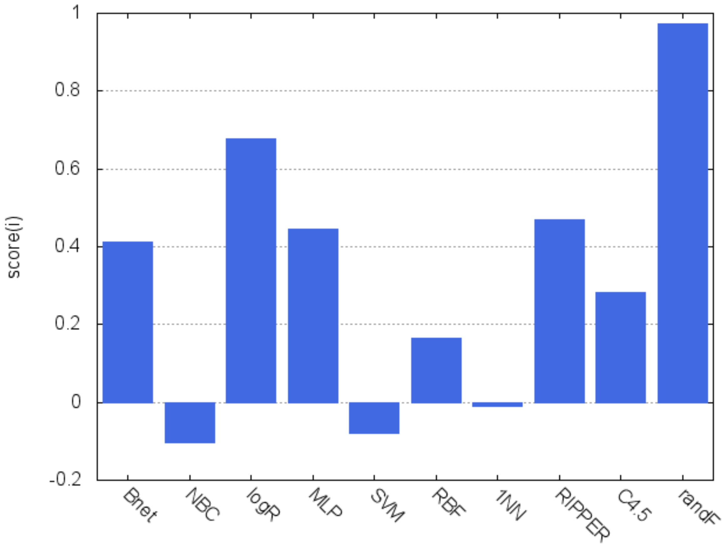
Despite the ranks achieved with TOPSIS and PROMETHEE being rather similar to one another, a composite ranking score was further defined as the mean of the preference values of both techniques for each prediction method i. This composite score allows for combining the preference rates R i + and ϕ ( a i ) of an alternative (prediction model) i in a fair manner as follows:
s c o r e ( i ) = R i + + ϕ ( a i ) 2 .
Furthermore, this score can be easily generalized to L different MCDM methods as:
G e n e r a l i z e d   s c o r e ( i ) = 1 L j L v a l u e j ,
where v a l u e j denotes the preference value given by the method j.
Figure 2 displays a graphical representation of the composite scores, which is a simple way of visualizing the rationale of the decisions made. It clearly shows that both random forest and logistic regression are superior to all the other classifiers and, on the other hand, the poor performance achieved by the naïve Bayes, SVM and 1NN algorithms is also apparent.

5. Conclusions

The present analysis supports the synergetic application of MCDM techniques for the performance assessment of credit granting decision systems. Through a series of experiments, it has been shown that the employment of an individual metric may give rise to inconsistent conclusions about what is the best prediction model for a given problem, which would lead to selecting an inappropriate method with not the most reliable results.
TOPSIS and PROMETHEE, which are two well-known MCDM techniques, have been tested in the experiments applying ten prediction models (alternatives) to six real-world bankruptcy and credit data sets and using seven performance evaluation criteria. The use of single performance metrics have designated different classifiers as the most suitable alternatives. These results suggest that credit granting decision corresponds to a real-world application where the MCDM techniques are especially useful to consistently assess a pool of classifiers and help decision-makers to choose the most beneficial model. In our experiments, both TOPSIS and PROMETHEE have determined that random forest and logistic regression are the best performing prediction methods on most of the performance evaluation measures.
Furthermore, we have also introduced a plain score that can be easily expressed as a linear combination of the preference values given by a number of MCDM methods. The most important advantages of this simple score are two-fold: (i) it converts the individual preference values of the MCDM models into a single scalar, thus allowing for making more trustworthy decisions; and (ii) it can be graphically represented for a better understanding of the decisions made.
In the experiments, we have tested 10 classification models using their default parameter values given in WEKA. It is known that some of these classifiers can yield widely different results depending on the value of their parameters (e.g., the kernel function used in SVM, or the number of decision trees in a random forest). As future work, a more exhaustive analysis of the optimal parameter values for the classification problem here addressed should be performed.

Author Contributions

Conceptualization, A.I.M. and V.G.; Methodology, A.I.M., V.G., and J.S.S.; Formal Analysis, A.I.M., V.G., and J.S.S.; Investigation, A.I.M., V.G., and J.S.S.; Resources, V.G. and J.S.S.; Data Curation, A.I.M. and V.G.; Writing—Original Draft Preparation, A.I.M.; Writing—Review and Editing, V.G. and J.S.S.; Supervision, J.S.S.; Funding Acquisition, J.S.S.

Funding

This research was funded by Universitat Jaume I Grant No. UJI-B2018-49.

Conflicts of Interest

The authors declare no conflict of interest.

References

  1. Lee, T.S.; Chiu, C.C.; Chou, Y.C.; Lu, C.J. Mining the Customer Credit Using Classification and Regression Tree and Multivariate Adaptive Regression Splines. Comput. Stat. Data Anal. 2006, 50, 1113–1130. [Google Scholar] [CrossRef]
  2. Shi, Y.; Peng, Y.; Kou, G.; Chen, Z. Classifying credit card accounts for business intelligence and decision-making: A multiple-criteria quadratic programming approach. Int. J. Inf. Technol. Decis. Mak. 2005, 4, 581–599. [Google Scholar] [CrossRef]
  3. Tseng, F.; Lin, L. A quadratic interval logit model for forecasting bankruptcy. Omega 2005, 13, 85–91. [Google Scholar] [CrossRef]
  4. Huang, Z.; Chen, H.; Hsu, C.J.; Chen, W.H.; Wu, S. Credit rating analysis with support vector machines and neural networks: A market comparative study. Decis. Support Syst. 2004, 37, 543–558. [Google Scholar] [CrossRef]
  5. Atiya, A. Bankruptcy prediction for credit risk using neural networks: A survey and new results. IEEE Trans. Neural Netw. 2001, 12, 929–935. [Google Scholar] [CrossRef]
  6. Bensic, M.; Sarlija, N.; Zekic-Susac, M. Modelling small-business credit scoring by using logistic regression, neural networks and decision trees. Intell. Syst. Account. Financ. Manag. 2005, 13, 133–150. [Google Scholar] [CrossRef]
  7. Du Jardin, P. Predicting Bankruptcy Using Neural Networks and Other Classification Methods: The Influence of Variable Selection Techniques on Model Accuracy. Neurocomputing 2010, 73, 2047–2060. [Google Scholar] [CrossRef]
  8. Kozeny, V. Genetic algorithms for credit scoring: Alternative fitness function performance comparison. Expert Syst. Appl. 2015, 42, 2998–3004. [Google Scholar] [CrossRef]
  9. Marqués, A.; García, V.; Sánchez, J. Two-level classifier ensembles for credit risk assessment. Expert Syst. Appl. 2012, 39, 10916–10922. [Google Scholar] [CrossRef]
  10. Tsai, C.F.; Wu, J.W. Using Neural Network Ensembles for Bankruptcy Prediction and Credit Scoring. Expert Syst. Appl. 2008, 34, 2639–2649. [Google Scholar] [CrossRef]
  11. Twala, B. Combining classifiers for credit risk prediction. J. Syst. Sci. Syst. Eng. 2009, 18, 292–311. [Google Scholar] [CrossRef]
  12. Wang, G.; Hao, J.; Ma, J.; Jiang, H. A comparative assessment of ensemble learning for credit scoring. Expert Syst. Appl. 2011, 38, 223–230. [Google Scholar] [CrossRef]
  13. Caruso, G.; Gattone, S.A.; Fortuna, F.; Di Battista, T. Cluster Analysis as a Decision-Making Tool: A Methodological Review. Decision Economics: In the Tradition of Herbert A. Simon’s Heritage; Bucciarelli, E., Chen, S.H., Corchado, J.M., Eds.; Springer International Publishing: Cham, Switzerland, 2018; pp. 48–55. [Google Scholar]
  14. Caruso, G.; Gattone, S.A.; Balzanella, A.; Di Battista, T. Cluster Analysis: An Application to a Real Mixed-Type Data Set. Models and Theories in Social Systems; Flaut, C., Hošková-Mayerová, Š., Flaut, D., Eds.; Springer International Publishing: Cham, Switzerland, 2019; pp. 525–533. [Google Scholar]
  15. Caruso, G.; Gattone, S.A. Waste management analysis in developing countries through unsupervised classification of mixed data. Soc. Sci. 2019, 8, 186. [Google Scholar] [CrossRef]
  16. Valls Mateu, A. ClusDM: A Multiple Criteria Decision Making Method for Heterogeneous Data Sets. Ph.D. Thesis, Universitat Politècnica de Catalunya, Barcelona, Spain, 13 December 2002. [Google Scholar]
  17. Baesens, B.; Gestel, T.V.; Viaene, S.; Stepanova, M.; Suykens, J.; Vanthienen, J. Benchmarking state-of-the-art classification algorithms for credit scoring. J. Oper. Res. Soc. 2003, 54, 627–635. [Google Scholar] [CrossRef]
  18. Min, J.; Lee, Y.C. Bankruptcy Prediction Using Support Vector Machine with Optimal Choice of Kernel Function Parameters. Expert Syst. Appl. 2005, 28, 603–614. [Google Scholar] [CrossRef]
  19. Trustorff, J.H.; Konrad, P.; Leker, J. Credit risk prediction using support vector machines. Rev. Quant. Financ. Account. 2011, 36, 565–581. [Google Scholar] [CrossRef]
  20. Desai, V.; Crook, J.; Overstreet, G. A comparison of neural networks and linear scoring models in the credit union environment. Eur. J. Oper. Res. 1996, 95, 24–37. [Google Scholar] [CrossRef]
  21. Yobas, M.; Crook, J.; Ross, P. Credit scoring using neural and evolutionary techniques. IMA J. Math. Appl. Bus. Ind. 2000, 11, 111–125. [Google Scholar] [CrossRef]
  22. Bhaduri, A. Credit scoring using artificial immune system algorithms: A comparative study. In Proceedings of the 2009 World Congress on Nature & Biologically Inspired Computing (NaBIC), Coimbatore, India, 9–11 December 2009; pp. 1540–1543. [Google Scholar]
  23. Antonakis, A.; Sfakianakis, M.E. Assessing naïve Bayes as a method for screening credit applicants. J. Appl. Stat. 2009, 36, 537–545. [Google Scholar] [CrossRef]
  24. Cohon, J. Multiobjective Programming and Planning; Dover Publishings: New York, NY, USA, 2004. [Google Scholar]
  25. Köksalan, M.; Wallenius, J.; Zionts, S. Multiple Criteria Decision Making: From Early History to the 21st Century; World Scientific: Singapore, 2011. [Google Scholar]
  26. Triantaphyllou, E. Multi-Criteria Decision Making Methods. In Multi-Criteria Decision Making Methods: A Comparative Study; Springer: Boston, MA, USA, 2000; Volume 44, pp. 5–21. [Google Scholar]
  27. Belton, V.; Stewart, T. Multiple Criteria Decision Analysis—An Integrated Approach; Kluwer Academic Publishers: Norwell, MA, USA, 2002. [Google Scholar]
  28. Pardalos, P.; Siskos, Y.; Zopounidis, C. Advances in Multicriteria Analysis; Kluwer Academic Publishers: Dordrecht, The Netherlands, 1995. [Google Scholar]
  29. Shih, H.S.; Shyur, H.J.; Lee, E. An extension of TOPSIS for group decision-making. Math. Comput. Model. 2007, 45, 801–813. [Google Scholar] [CrossRef]
  30. Hwang, C.L.; Yoon, K. Multiple Attribute Decision Making—Methods and Applications; Springer: New York, NY, USA, 1981. [Google Scholar]
  31. Yoon, K.; Hwang, C.L. Multiple Attribute Decision Making: An introduction; SAGE Publications: Thousand Oaks, CA, USA, 1995. [Google Scholar]
  32. Brans, J.P.; Vincke, P. A Preference Ranking Organisation Method: The PROMETHEE Method for Multiple Criteria Decision-Making. Manag. Sci. 1985, 31, 647–656. [Google Scholar] [CrossRef]
  33. Brans, J.P.; Mareschal, B. PROMETHEE methods. In Multiple Criteria Decision Analysis: State of the Art Surveys; Springer: Boston, MA, USA, 2005; pp. 163–186. [Google Scholar]
  34. Jablonsky, J. Software support for multiple criteria decision-making problems. Manag. Inf. Syst. 2009, 4, 29–34. [Google Scholar]
  35. Hall, M.; Frank, E.; Holmes, G.; Pfahringer, B.; Reutemann, P.; Witten, I. The WEKA data mining software: An update. SIGKDD Explor. Newsl. 2009, 11, 10–18. [Google Scholar] [CrossRef]
  36. Sabzevari, H.; Soleymani, M.; Noorbakhsh, E. A comparison between statistical and data mining methods for credit scoring in case of limited available data. In Proceedings of the 3rd CRC Credit Scoring Conference, Edinburgh, UK, 4 November 2007. [Google Scholar]
  37. Pietruszkiewicz, W. Dynamical Systems and Nonlinear Kalman Filtering Applied in Classification. In Proceedings of the 7th IEEE International Conference on Cybernetic Intelligent Systems, London, UK, 9–10 September 2008; pp. 263–268. [Google Scholar]
  38. Thomas, L.; Edelman, D.; Crook, J. Credit Scoring and Its Applications; SIAM: Philadelphia, PA, USA, 2002. [Google Scholar]
  39. Alfaro, E.; García, N.; Gámez, M.; Elizondo, D. Bankruptcy forecasting: An empirical comparison of AdaBoost and neural networks. Decis. Support Syst. 2008, 45, 110–122. [Google Scholar] [CrossRef]
  40. Hand, D. Good practice in retail credit scorecard assessment. J. Oper. Res. Soc. 2005, 56, 1109–1117. [Google Scholar] [CrossRef]
  41. Abdou, H.; Pointon, J. Credit scoring, statistical techniques and evaluation criteria: A review of the literature. Intell. Syst. Account. Financ. Manag. 2011, 18, 59–88. [Google Scholar] [CrossRef]
  42. Lee, J.S.; Zhu, D. When Costs Are Unequal and Unknown: A Subtree Grafting Approach for Unbalanced Data Classification. Decis. Sci. 2011, 42, 803–829. [Google Scholar] [CrossRef]
  43. Sokolova, M.; Lapalme, G. A systematic analysis of performance measures for classification tasks. Inf. Process. Manag. 2009, 45, 427–437. [Google Scholar] [CrossRef]
  44. Japkowicz, N.; Shah, M. Evaluating Learning Algorithms: A Classifier Perspective; Cambridge University Press: New York, NY, USA, 2011. [Google Scholar]
  45. Wang, T.C.; Lee, H.D. Developing a fuzzy TOPSIS approach based on subjective weights and objective weights. Expert Syst. Appl. 2009, 36, 8980–8985. [Google Scholar] [CrossRef]
  46. Deng, H.; Yeh, C.H.; Willis, R.J. Inter-company comparison using modified TOPSIS with objective weights. Comput. Oper. Res. 2000, 27, 963–973. [Google Scholar] [CrossRef]
  47. Lee, T.S.; Chen, I.F. A two-stage hybrid credit scoring model using artificial neural networks and multivariate adaptive regression splines. Expert Syst. Appl. 2005, 28, 743–752. [Google Scholar] [CrossRef]
Figure 1. Diagram of the 5-fold cross-validation method (blocks in blue represent the testing folds at each step).
Applsci 09 05052 g001
Figure 2. Composite ranking scores.
Applsci 09 05052 g002
Table 1. Decision matrix for a general MCDM problem ( z i j denotes the value of alternative a i assessed by criterion c j ).
c 1 c 2 c N
a 1 z 11 z 12 z 1 N
a 2 z 21 z 22 z 2 N
a M z M 1 z M 2 z M N
Table 2. Parameter values of the classifiers.
ModelParameters
BnetInitial count for estimating the conditional probability tables of the Bayes network = 0.5; Naive Bayes network used as the initial structure; K2 hill climbing algorithm for structure learning; Bayesian Dirichlet score to evaluate the structure learned
MLPBroyden–Fletcher–Goldfarb–Shanno optimization algorithm; Sigmoid transfer function; Learning rate = 0.3; Momentum = 0.2; Maximum number of training epochs = 500; Neurons in the hidden layer = 2
RBFNormalized Gaussian RBF; Center vectors of the functions determined using K-means clustering
logRMultinomial logistic regression; Quasi-Newton optimization method; Ridge value in the log-likelihood = 1.0 × 10 8
SVMLinear kernel; Soft margin constant = 1.0: Tolerance = 0.001; Round-off error ϵ = 1.0 × 10 12 ; Sequential minimal optimization algorithm
1NNEuclidean distance
RIPPERNumber of folds = 3 (one fold is used for pruning, the rest for growing the rules); Minimum total weight of the instances in a rule = 2.0; Number of optimization runs = 2
C4.5Number of folds = 3 (one fold is used for pruning, the rest for growing the tree); Minimum number of instances per leaf = 2; Error-based pruning; Pruning confidence factor = 0.25
randFNumber of trees = 100; Number of randomly chosen attributes at each node = log 2 ( D ) + 1
Table 3. Overview of the databases used in the experiments.
#Variables#Positive#Negative#InstancesIR
Australian143073836000.80
sabiSPQ164724729441.00
Polish301281122401.14
German2470030010002.33
Thomas1290232312252.79
Iranian2795050100019.00
Table 4. Confusion matrix for a two-class problem.
Predicted Class
True classTrue-positive (TP)False-negative (FN)
False-positive (FP)True-negative (TN)
Table 5. Performance results for the Australian database.
AccRMSETP-RateTN-RateAUCTN-RateF-Measure
Bnet0.850.340.810.890.910.850.85
NBC0.770.440.590.920.890.740.76
logR0.870.320.880.860.930.870.87
MLP0.830.380.820.840.900.830.83
SVM0.860.380.930.800.860.860.86
RBF0.810.360.730.890.900.810.81
1NN0.810.430.800.830.810.810.82
RIPPER0.870.340.840.890.880.860.87
C4.50.860.360.830.880.860.850.86
randF0.870.310.870.870.930.870.87
Table 6. Performance results for the sabiSPQ database.
AccRMSETP-RateTN-RateAUCG-MeanF-Measure
Bnet0.890.330.800.980.930.890.89
NBC0.870.360.770.980.900.870.87
logR0.890.300.850.940.930.890.89
MLP0.850.340.780.920.900.850.85
SVM0.780.470.750.810.780.780.78
RBF0.780.390.580.990.830.760.78
1NN0.770.480.750.790.770.770.77
RIPPER0.890.300.810.970.920.890.89
C4.50.870.330.840.910.900.870.87
randF0.900.270.850.950.950.900.90
Table 7. Performance results for the Polish database.
AccRMSETP-rateTN-rateAUCG-meanF-measure
Bnet0.730.490.710.760.820.730.73
NBC0.690.530.890.460.750.640.67
logR0.740.440.760.710.810.730.74
MLP0.740.450.810.650.810.730.74
SVM0.710.540.670.750.710.710.71
RBF0.710.430.800.620.800.700.71
1NN0.750.500.770.730.750.750.75
RIPPER0.740.440.760.710.770.730.74
C4.50.690.490.670.710.710.690.69
randF0.790.390.830.740.860.780.79
Table 8. Performance results for the German database.
AccRMSETP-rateTN-rateAUCG-meanF-measure
Bnet0.720.430.850.420.740.600.71
NBC0.760.420.860.510.790.660.75
logR0.770.400.890.500.790.670.76
MLP0.710.510.790.530.740.650.71
SVM0.770.480.900.470.680.650.76
RBF0.730.420.840.480.740.630.72
1NN0.670.580.760.450.610.580.67
RIPPER0.730.440.870.400.640.590.71
C4.50.720.480.830.460.670.620.72
randF0.760.400.910.410.780.610.74
Table 9. Performance results for the Thomas database.
AccRMSETP-RateTN-RateAUCG-MeanF-Measure
Bnet0.740.440.970.100.600.310.67
NBC0.630.510.690.460.600.560.65
logR0.740.430.970.100.630.310.66
MLP0.740.440.930.200.700.430.69
SVM0.740.521.000.000.500.000.63
RBF0.730.440.980.020.590.140.63
1NN0.660.590.770.340.560.520.66
RIPPER0.730.440.940.150.550.380.68
C4.50.720.440.940.130.570.350.67
randF0.730.440.910.220.640.450.69
Table 10. Performance results for the Iranian database.
AccRMSETP-RateTN-RateAUCG-MeanF-Measure
Bnet0.950.230.990.020.720.140.93
NBC0.240.870.200.900.600.420.32
logR0.940.230.990.020.710.140.94
MLP0.930.240.970.200.700.440.93
SVM0.950.221.000.000.500.000.93
RBF0.950.221.000.000.610.000.93
1NN0.930.270.960.320.640.550.93
RIPPER0.940.230.990.040.520.200.92
C4.50.940.230.990.100.570.310.93
randF0.950.210.990.160.790.400.94
Table 11. Performance results averaged across the six experimental databases.
AccRMSETP-RateTN-RateAUCG-MeanF-Measure
Bnet0.810.380.860.530.790.590.80
NBC0.660.520.670.710.760.650.67
logR0.830.350.890.520.800.600.81
MLP0.800.390.850.560.790.660.79
SVM0.800.440.880.470.670.500.78
RBF0.790.380.820.500.750.510.76
1NN0.770.480.800.580.690.660.77
RIPPER0.820.370.870.530.710.610.80
C4.50.800.390.850.530.710.620.79
randF0.830.340.890.560.830.670.82
Weight0.027620.200480.085240.042860.219540.215710.20855
Table 12. Preference rankings given by TOPSIS and PROMETHEE.
TOPSISPROMETHEE
AlternativeRank R i + Rank ϕ ( a i )
Bnet(4)0.76538(5)0.05905
NBC(10)0.17492(8)−0.38273
logR(2)0.87375(2)0.48095
MLP(6)0.70375(3)0.18736
SVM(8)0.44787(10)−0.60858
RBF(5)0.71332(9)−0.38358
1NN(9)0.31014(7)−0.32921
RIPPER(3)0.80342(4)0.13517
C4.5(7)0.70363(6)−0.13937
randF(1)0.96282(1)0.98095

