Evaluation of Loading Bay Restrictions for the Installation of Offshore Wind Farms Using a Combination of Mixed-Integer Linear Programming and Model Predictive Control

Featured Application

This article demonstrates a combination of Mixed-Integer Linear Programming with methods usually applied for short-term control, namely the Model Predictive Control scheme, to achieve decision support for the scheduling of installation activities for offshore wind farms. The general approach applies to several areas of application, where time-dependent uncertainties complicate mid- to long-term planning.

Abstract

The installation of offshore wind farms poses particular challenges due to expensive resources and quickly changing weather conditions. Model-based decision-support systems are required to achieve an efficient installation. In the literature, there exist several models for scheduling offshore operations, which focus on vessels but neglect the influence of resource restrictions at the base port and uncertainties involved with weather predictions. This article proposes a Mixed-Integer Linear Programming model for the scheduling of installation activities, which handles several installation vessels as well as restrictions about available cargo bridges at the port. Additionally, the article explains how this model can be combined with a Model Predictive Control scheme to provide decision support for the scheduling of offshore installation operations. The article presents numerical studies of the effects induced by resource restrictions and of different parametrizations for this approach. Results show that even small planning windows, paired with comparably low computational times, achieve reasonably good results. Moreover, the results show that an increase in vessels comes at diminishing returns concerning the installation efficiency. Therefore, the results indicate that available good-weather windows primarily limit efficiency.

1. Introduction

Wind energy constitutes one of the most promising technologies to cover the world’s need for sustainable energy. In 2017, wind farms with a capacity of around 52 Gigawatts were constructed worldwide, increasing the total amount of energy produced by wind turbines by approximately 11% to a total of 539 Gigawatts [1]. As a result of high wind speeds at sea, offshore wind farms can produce large amounts of energy [2,3]. According to the Renewables 2018 Status Report [1], the amount of energy generated by offshore wind farms was exponentially increasing over the last decade. While offshore wind farms provide a steadier stream of energy at higher rates compared to onshore wind farms, their construction poses particular challenges due to their increased weight and dimensions. Also, the installation process requires highly specialized, expensive vessels, and resources [4,5]. In general, logistics costs during the installation can amount to about 15% to 20% of the costs for offshore wind farms [6,7,8]. As a result, the efficient use of available resources constitutes a predominant factor of success. On the one hand, this requires optimal planning and scheduling of available resources; on the other hand, highly dynamic weather conditions at sea render the execution of such plans difficult. Consequently, adaptive, model-based decision-support systems can be used to achieve optimal planning while retaining a high degree of adaptability to these dynamic conditions [9]. Most of the models found in the literature focus on the simulation or scheduling of offshore operations, using a provided set of vessels. These models are often used to evaluate different amounts of vessels, e.g., [10,11]. Nevertheless, efficient use of vessels also requires considering the availability of resources at the base port. For example, loading components for an offshore wind turbine at port takes several hours per part, approximately amounting to a total of 12 h per turbine. If only a single loading bay is available, this long duration can quickly render port operations to become a bottleneck if several vessels are applied. As companies usually charter vessels and bays for extended periods, optimization models should be capable of handling such restrictions. Unfortunately, current models do not include restrictions on loading bays, which could render their results inaccurate and lead to an underestimation of the project duration. In turn, such underestimations may result in delays and, thus, in high additional costs and the need for rescheduling. Moreover, current models generally try to optimize the overall project with a more or less unlimited prediction horizon. Such long horizons require exact and reliable long-term weather forecasts, which are not available in reality.

This article extends the Mixed-Integer Linear Programming (MILP) optimization model and the overall Model Predictive Control (MPC)-based approach presented in [9] to handle several vessels and different numbers of loading bays to achieve more realistic plans under forecast uncertainties. Additionally, it presents an enhanced method to preprocess weather forecast uncertainties for their use during the optimization. The MILP model still aims to find optimal schedules for previously decided numbers of vessels and bays but can provide a foundation to optimize these numbers in future work. In this context, the article also describes significant extensions to the MPC-based methodology to enable usage of the extended optimization model as decision support under weather forecast uncertainties by deriving plans incrementally. Finally, this article provides numeric studies of different configurations with regards to vessels and bays, to assess the impact of loading restrictions on the performance of the installation process as well as to evaluate the extended approach in general.

The next Section 1.1 presents a description of the installation process and its characteristics. The article then follows with an overview of the relevant literature concerning the scheduling for the installation of offshore wind farms (Section 1.2) and by presenting general scheduling approaches in Section 1.3 and Section 1.4. Afterward, Section 2 presents the overall methodology and details its single steps. This section also includes the extended Mixed-Integer model in Section 2.4. Finally, Section 3 details the experimental setup and the numerical results. The article closes with a conclusion and a description of future work (Section 4).

1.1. Installation Process for Offshore Wind Farms

According to Vis and Ursavas [12] and Quandt et al. [13], the installation process comprises three main stages: First, the construction of foundations and the connection to the energy grid. Second, the installation of top structures. Third, the ramp-up and commissioning. Commonly, different companies take responsibility for the first stage and the remaining two stages of the process. Generally, these tasks proceed sequentially: First, one company installs the foundations and cables, and afterward, often in the following year, another company installs and commissions the wind turbines. While the components and resources in the first and second stages differ, the overall process remains the same.

In the literature, authors have proposed two different types of installation concepts: The conventional concept, as depicted in Figure 1, and feeder-based concepts. These concepts mainly differ in how installation vessels are applied. For the conventional concept, these vessels travel between the base port and the installation site, while feeder-based concepts try to avoid these tours by applying specific feeder vessels. For more information in feeder-based concepts, refer to [14] or [15]. The conventional concept assumes that the base-port buffers the components before installation. So-called heavy-lift vessels perform the transport from production sites to the base port as these vessels usually come at comparably low charter rates. During the construction process, more expensive installation vessels pick up these components from the port, travel to the installation site, and perform construction there. The same process applies to the construction of founding structures. Similarly, the components are transported by heavy-lift vessels to the base port. In contrast to the installation of top structures, the installation of founding structures involves two different types of vessels, i.e., specially equipped installation vessels, and so-called cable vessels.

In general, the installation requires several types of vessels. While so-called heavy-lift vessels do not provide any special equipment, they usually have large transportation capacities. Generally, these vessels have comparably low charter rates of about €10,000 to €20,000 a day [17]. Specially equipped installation and cable vessels conduct the construction of founding structures. These installation vessels, so-called jack-up vessels, can be equipped with different tools. As an example, hydro hammers are a standard tool for the installation of founding structures. Cable vessels are used to mount and lay cables between the turbines and the offshore network hubs to establish a connection to the power grid. During the installation, jack-up vessels are usually equipped with a crane to perform installation operations. Moreover, these vessels use retractable pillars, to mount themselves above the sea level. Therefore, the pillars are lowered into the seabed until the vessel rises out of the ocean. This jack-up operation is generally used to steady the vessels, enabling the vessel to conduct installation operations even under comparably rough sea conditions. These jack-up vessels come at high charter rates of between €70,000 and €145,000 a day [17].

As the planning problem for foundations and top structures is more or less identical, this article uses the actual turbines as an example. Their installation is performed sequentially, generally in a single session [9]. Therefore, the installation vessel first positions itself next to the foundation and performs its jack-up operation. Afterward, the components are assembled from bottom to top, in the order of tower, nacelle, blades, and finally, the connecting hub. After completing the installation, the vessel jacks-down again. Afterward, it moves to the next foundation or back to the base port. It is to mention that after jacking-up close to one position, installation vessels remain stationary until they finished installing all components. In practice, a single position should only be used once for jacking-up to avoid damaging the foundations or even the installation vessel itself, as the jack-up process punctures and loosens the seabed.

Each of the listed offshore operations is restricted by specific weather conditions, given by maximum wind speeds and maximum wave heights. If the current weather conditions do not meet these requirements for the full duration of an operation, it cannot be conducted for safety reasons or has to be aborted to avoid danger to the staff, already installed turbine parts, or the components currently being handled. Aborting an operation, thereby leads to a loss of all current progress. Consequently, weather dynamics can easily result in expensive waiting times for the installation vessel, leading to high, unplanned costs. Moreover, charter contracts often set different prices for vessels being in port and for the vessel to be offshore, which, on average, differ by approximately 30% [9]. As a result of these weather restrictions, installation activities commonly take place in the months April until October to ensure a sufficient amount of good-weather windows.

As can be deducted from the process description, efficient scheduling of installation operations is a significant cost factor for this process. The state of the art also supports this conclusion. Most of the presented models deal with the scheduling of installation vessels in one way or another (compare Section 1.2). Weather dynamics are the major influential factor in the scheduling: Only if the weather is good enough, turbines can be installed quickly to avoid expensive waiting times.

Nevertheless, to conduct an installation of an offshore wind turbine (OWT), the required components need to be loaded into the jack-up vessel in advance. As given in

Table 1. Duration of basic operations.

Operation	Base Duration (h)	Max. Wind (m/s)	Max. Wave (m)
Traveling	4	21	2.5
Positioning	1	14	2
Jack-up/-down	2	14	1.8
Load Tower	3	12 ⋆	5 ⋆
Load Nacelle	2	12 ⋆	5 ⋆
Load Blade	2	10 ⋆	5 ⋆
Load Hub	1	12 ⋆	5 ⋆
Install Tower	3	12	2.5 †
Install Nacelle	3	12	2.5 †
Install Blade	2	10	2.5 †
Install Hub	2	12	2.5 †

⋆ Omitted using loading bridges. † Unaffected by wave height due to jack-up.

, loading a complete set of components takes up around 12 h, whereas the installation itself amounts to 19 h in the best case. The table lists operations used in this article’s planning model. Therefore, the column Base Duration refers to the minimum time required to conduct the operation, if the current weather conditions do not exceed the limits given in the columns Max. Wind and Max. Wave for the full base duration. As can be seen, most operations are affected by high wind speeds as they involve the use of a crane. In contrast, most operations omit the influence of the wave height due to the jack-up, which keeps the vessel steady. Moreover, the values given in this table assume that the base port is a controlled environment and that loading bridges are used to omit the influence of wind and waves. The limits and durations in Table 1 closely follow the information provided in [9] and [15] to represent realistic assumptions. Within the literature, other, usually softer bounds, can be found too (compare [5] for a review of the overall planning problem).

As a consequence of the weather dependency, an accurate mid- to long-term planning can only rely on weather forecasts. Unfortunately, with an increasing prediction horizon, these forecasts tend to become increasingly uncertain. According to the Deutscher Wetterdienst, current models achieve an accuracy of approximately 75% for a prediction horizon of 168 h (one week) [18]. For horizons of two weeks, an average accuracy of approximately 35% can be assumed, indicating an increasing decline in accuracy with increasing horizons. As a result, an operative decision-support system cannot provide plans for very long prediction horizons. While the state of the art presented in the next section demonstrates that historical weather records can be used to achieve accurate long-term estimations, a decision-support tool for the operative scheduling has to rely on an incremental approach to be useful in practice. From information gathered in talks with other researchers in this field, it became apparent that in practice, the scheduling is performed more or less ad-hoc. Therefore, the vessels’ captains and the port-side operations managers continuously render decisions based on experience, current weather conditions, and using forecasts.

Hazir provides a review of models and approaches for decision-support systems for the monitoring and control of projects in general. Therefore he defines the main tasks of decision-support systems as the identification and reporting of the project’s current status, the comparison with a predefined plan, the identification of and analysis of deviations, and finally, the implementation of countermeasures [19]. A decision-support system provides two main functionalities to achieve this objective: First, a monitoring policy, defining which information must be collected and monitored, also defining the when and how. Second, an intervention and control policy, which clearly states who should counteract deviations from the provided plan, when and in which way.

1.2. Planning Approaches for the Installation of Offshore Wind Farms

In current literature, only a few works deal explicitly with the installation planning of offshore wind farms [5,12]. In general, these approaches can be classified in either simulation-based approaches, used to evaluate given configurations, or in optimization-based approaches, aiming to generate optimized plans for certain aspects of the overall planning problem.

In terms of simulation-based models, all current approaches focus on the evaluation of the involved actors’ behavior, usually concentrating on vessels, in terms of the overall installation performance. Muhabie et al. present an approach to compare the effect of deterministic and stochastic assumptions concerning weather conditions [8]. Vis et al. propose a simulation model to evaluate different pre-assembly strategies and to assess their impact on the overall installation process [12]. Ait-Alla et al. propose a multi-agent-based model to compare the conventional installation concept with feeder concepts, later extending the simulation model for different feeder concepts [14,15]. While all these approaches simulate the behavior of vessels and thus can be used to derive a plan after the simulation finished, they do not include an optimization component to evaluate different schedules or configurations. Whereas most of these models include storage capacity limitations, it is not explicitly stated or investigated, if the used simulation models support constraining operative resources at the base port.

In terms of mathematical models, the majority of literature focuses on the generation of plans on different levels of abstraction. Therefore, most authors use Mixed-Integer Linear Programming formulations to tackle their optimization problem. Kerkhove et al. apply a heuristic approach to plan the deployment and decommissioning of vessels, thereby optimizing the overall cost of the installation process [20]. Scholz-Reiter et al. combine a precedence-based job-shop scheduling formulation with a multi-periodic production formulation to derive optimal plans for small scenarios with a daily resolution [21]. Later, they extend this model by heuristics to enable solving larger problem instances [22]. The same model was recently extended by Ursavas et al. to deal with probabilistic weather assumptions [23]. Besides their multi-agent-based approach, Ait-Alla et al. propose another Mixed-Integer model, which closely resembles a time-indexed job-shop formulation [10]. For each indexed period of 12 hours, the optimizer determines the number of foundations, cables, and top structures to be built using a predefined vessel configuration. Irawan et al. propose a bi-objective, Mixed-Integer optimization model, aiming to find a trade-off between minimal construction times and minimal costs [11]. The authors recently extended this model for the decommissioning of offshore wind farms in [24].

As can be seen from these descriptions, most optimization models focus on the handling of vessels, operations, and weather conditions. Only a few models include port-related features [25], again, only focusing on port storage capacities. The mentioned models do not cover the availability of supporting resources such as loading bays and stationary cargo bridges. Moreover, the majority of the presented models try to achieve schedules for the overall installation project and thus assume that weather conditions are known a-priori. As described in the process description and the state of the art, historical information can be used to achieve reasonable estimations, but are not suitable to support the operative decision-making process, as they are not designed to handle dynamic weather conditions at sea. In terms of decision-support systems, current approaches are monolithic per design, i.e., they derive the complete plan once, and do not perform any iterations or increments during the execution. Thus, there exist no monitoring or intervention policies.

1.3. General Classes of Scheduling Problems

As can be seen from the process description and the description of current planning methods for offshore installations, the problem generally resembles a sub-type of a scheduling problem. Therefore, a fixed number of jobs, consisting of sequential operations, is assigned to a defined number of capable machines. In this context, the most commonly used objective function is the minimization of the makespan, i.e., the time that is needed to complete all jobs [26]. When compared to this classical notion, installation operations resemble machining operations, and vessels represent machines. As there is no inherently fixed sequence between vessels (machines) as typical to flow shop scenarios, the overall structure resembles a job-shop scheduling problem (JSSP). This class of problems is strongly NP-hard, even NP-complete for three or more machines [27]. Thus, an optimizer cannot guarantee the optimality of a solution in polynomial time, even for small scenarios. For this reason, this class is denoted as NP for non-polynomial. As a result, a multitude of solution algorithms has been proposed, ranging from exact mathematical models to heuristic or metaheuristic approaches. Please refer to Zhang et al. [28] for a concurrent review of solution approaches. Within the literature, there exist several classifications of sub-types of the JSSP, e.g., [28,29,30]. Nevertheless, besides giving a broad list of possible classifications, Zhang et al. propose four predominant sub-types for JSSP [28]:

Basic JSSP: 

The Basic JSSP constitutes the simplest class of job-shop scheduling problems. The Basic JSSP assumes that each operation can only be conducted by a single machine, thus resulting in a sequencing problem.

Flexible JSSP: 

The Flexible JSSP extends the basic formulation by allowing a specified set of alternative machines to perform operations. This flexibility increases the problem’s complexity: In addition to the already present sequencing problem (order of operations per machine), the Flexible JSSP also has to cope with an additional routing problem, deciding which machine to choose for which operation [26].

Multi-Resource JSSP: 

The Multi-Resource JSSP extends the formulation of the Flexible JSSP by another dimension. In addition to the machine, each operation additionally requires other limited resources. These could, for example, be workers, tools, or dies.

Multi-Plant Multi-Resource JSSP: 

This type of model extends the Multi-Resource JSSP by regarding multiple plants or production facilities. Therefore, it is also necessary to include the transport of orders between those facilities within the scheduling.

Depending on the scope of the offshore installation problem considered, the installation planning can either be classified as Flexible JSSP or even as Multi-Resource Flexible JSSP if including crew- and personnel-assignments in the model. Nevertheless, from the process description, it can be argued that the three stages of the installation process, i.e., foundations, turbines, and commissioning, can be considered to be individual, sequentially performed tasks. Therefore, crew management primarily becomes an issue for the commissioning stage of the installation process [5]. As a result, this article considers the operative installation planning of offshore wind farms in terms of a Flexible JSSP. This classification is justified, as, e.g., installation vessels can perform overlapping sets of operations. For example, all installation vessels can perform all assembly operations, leading to a so-called Complete Flexible JSSP, where multiple machines offer the same sets of operations. If also considering transport operations by heavy-lift or feeder vessels, overlaps of performable operations exist, resulting in a so-called Partial Flexible JSSP. Please refer to Zhang et al. [28] for more information on Partial and Complete Flexible JSSPs and a more detailed definition of the different sub-types.

Literature proposes a multitude of models for Flexible JSSP. Nevertheless, these usually follow one of three basic types of formulations. In this context, Demir and İs̨leyen present an overview of these base formulations and compare different implementations against each other, concerning their optimality and CPU time [31]:

Time-Indexed formulation: 

These types of models index the generated schedules over discrete time instances, e.g., minutes or hours. Therefore, the schedules denote for each machine and each time instance, which operation of which job is currently processed. The drawback of these formulations is the high number of decision variables, which is at least quadratic over the number of machines and time instances. According to Demir and İs̨leyen [31], a significant drawback of these formulations is that the planning horizon must be estimated in advance so that the optimizer can schedule all operations.

Sequence-Position formulations: 

This type of formulation uses discrete slots instead of time instances, which refer to semantic concepts, e.g., to machining operations. Therefore, it represents each machine by a sequence of slots, assigning operations to them. This type of formulation closely resembles a time-indexed formulation but reduces the number of decision variables by summarizing these into discrete slots of equal length in time. For example, if a machine performs three operations of lengths 2 h, 2.5 h, and 3 h, a formulation of this class would most probably use slots of 3 h length. As a trade-off, this abstraction reduces the resolution of the model (for the example above by factor 3 compared to an hourly time-indexed model) but may lead to weaker solutions, e.g., if operations finish in less time than assigned to a sequencing slot. These formulations require an a-priori estimation of the number of slots to allow the optimizer to schedule all operations. Consequently, this class summarizes all indexed formulations, which do not focus on single time instances but higher-level concepts. This reduces the complexity and simplifies the formulation of semantic constraints, e.g., like not assigning a morning shift directly after a night shift.

Precedence-based formulations: 

In contrast to the formulations above, precedence-based models use a continuous representation of time. Therefore, the generated solutions are indexed over the number of operations to be performed, usually resulting in fewer decision variables. The schedules denote start or end times, and the assigned machine for each operation.

In addition to the formulation itself, the environment poses an essential factor for the choice of approaches. Therefore, several authors, e.g., [28,32], include the differentiation into static and dynamic JSSPs. In static scenarios, all variables and conditions are known a-priori. In contrast, dynamic scenarios include various kinds of dynamics like, e.g., variable processing times, machine breakdowns, or rush orders.

1.4. Dynamic Scheduling Approaches

While the formulations and models described in the last subsection can derive optimal schedules for a provided system, weather dynamics require dynamic approaches to cope with the associated uncertainties. Several authors provide a review of current methods for the dynamic scheduling in production environments, e.g., [32,33,34]. Therefore, they provide a more or less common classification of these approaches, which is summarized below:

Reactive and Continuous Approaches: 

Reactive approaches generally do not incorporate uncertainties into the initial planning but rely on so-called recourse actions in cases of plan failures, i.e., a rescheduling. Therefore, some authors distinguish between approaches that only react to disturbances and between approaches that perform a continuous rescheduling. The first class of reactive approaches mostly focuses on a reduction of rescheduling times, e.g., by only selecting affected operations or by applying dispatching rules. The second class often uses receding horizon techniques (e.g., variations of the Model Predictive Control) and combines these with state-space descriptions to avoid expensive optimizations.

Preventive (Robust and Stochastic) Approaches: 

Preventive approaches try to provide schedules that can cope with the dynamics of the system in general. At this, the plans are generally designed to either focus on the worst possible case (robust plans) or to provide alternatives for possible scenarios using stochastic programming techniques. In general, robust plans tend to be too conservative as they usually assume the worst case. In contrast, stochastic plans come at very high computational costs, as the solver needs to compute alternative plans for different probable cases in advance.

Predictive-Reactive Approaches: 

This class of approaches tries to assume the extent of disturbances during the initial planning stage and employ reactive recourse actions if additional disturbances occur. Dias and Ierapetritou provide the example of fuzzy-based approaches, which translate uncertainties into a fuzzy description of the resulting variables. These descriptions are then used to derive schedules [34]. This type of reformulation enables a reduction of the models’ complexity as done for robust scheduling approaches, but does not limit the results to the worst case. Ouelhadj and Petrovic provide an overview of approaches, which use a bi-objective formulation, minimizing the makespan, and the impact of disturbances on the overall plan [33].

1.5. Summary of the Research Aim and the Assumptions

The provided state of the art demonstrates that the scheduling of offshore operations during the installation constitutes a crucial but hard-to-achieve task. On the one hand, it involves expensive resources, which must be chartered long before the actual project starts. On the other hand, offshore operations subject to highly dynamic weather conditions, which render accurate long-term planning impossible. This article aims to provide a methodology that can act as a basis for a decision-support system for the scheduling of offshore operations. In contrast to the approaches found in the literature, the proposed approach combines Mixed-Integer Linear Programming to achieve optimal plans with a Model Predictive Control scheme to handle the involved dynamics. Current approaches found in the literature usually entirely rely on optimization, which, in practice, would require perfect data, or use reactive approaches in their simulation, which usually results in sub-optimal plans. Compared to previous work, this article extends the proposed methodology to handle several vessels and port-site resource restrictions. Moreover, it presents a novel approach to discretize weather dynamics based on Markov Chains.

The overall installation consists of three distinct, consecutive stages. Due to the consecutiveness, this article considers these stages as disjunct scheduling problems. These stages only differ in their parametrization. Thus, the article chooses the installation of top structures as an example, as it contains the most complex sequence of operations. All experiments subject to the following assumptions:

• Each scenario only considers the actual installation part of the given supply chain. Consequently, this article assumes that components are always available at the base port.
• As in practice, this article only considers the so-called season from April to October, as it provides suitable weather conditions to perform offshore operations.
• If a scenario applies several installation vessels, all installation vessels are considered to be equal.
• The number of installation vessels is fixed for each scenario.
• The number of loading bays is fixed for each scenario.
• This article assumes that vessels host several crews to assure the availability of personnel seven days a week in three shifts (24 h).
• This article does not include staff planning and thus neglects differences in labor costs for night shifts or weekend shifts.

1.6. Notation

Table 2. Parameters and Variables used in the extended Mixed-Integer Linear Program.

Indices:
k, v, o	Indices	Indices for Time Instances (k), Vessels (v), and Operations (o) with $\mathit{k},\mathit{v}\in {\mathbb{N}}^{+}$ and $\mathit{o}\in \{1,2,3,4\}$.
Parameters determined a-priori:
N	Integer	Length of the prediction horizon as $N=P*T$
T	Integer	Sampling step size
P	Integer	Number of planning periods considered by the MILP
V	Integer	Number of installation vessels
$CAP$	Integer	Maximum loading capacity for vessels
$BAYS$	Integer	Number of loading bays
$D_{o,k}$	Integer	Estimated duration of operation o at time instance k
${START}_v$	Integer	Index of time instance when a vessel v is available
${INUSE}_k^{bays}$	Integer	Denotes the number of busy loading bays for each time instance k
$C_v^o$	Float	Cost for being offshore per hour by vessel v
$C_v^m$	Float	Cost for moving between port and site by vessel v
$C_v^p$	Float	Cost for port operations per hour by vessel v
$B^{owt}$	Float	Benefit for installing a turbine
$B^{early}$	Float	Benefit for finishing an operation early
Decision variables (start of operation events):
$Y_{v,k}^{owt}$	Binary	Denotes if a vessel v starts an installation operation at time instance k
$Y_{v,k}^{load}$	Binary	Denotes if a vessel v starts a loading operation at time instance k
$Y_{v,k}^{toPort}$	Binary	Denotes if a vessel v starts to move to the port at time instance k
$Y_{v,k}^{toSite}$	Binary	Denotes if a vessel v starts to move to the construction site at time instance k
Support variables (ongoing operations and states):
$X_{v,k}^{cap}$	Integer	Amount of currently loaded components
$Y_{v,k}^{loc}$	Binary	Denotes if vessel v is in port (0) or offshore (1)
$Y_{v,k}^{busy}$	Binary	Denotes if vessel v is currently performing an operation (1) or is idle (0)
$Y_{v,k}^{atBay}$	Binary	Denotes if vessel v is currently using a loading bay (1) or not (0)
$X_{v,k}^{fOwt}$	Integer	Denotes at which time instance an installation operation conducted by vessel v and started at instance k will finish
$X_{v,k}^{fOp}$	Integer	Denotes at which time instance a non-installation operation conducted by vessel v and started at instance k will finish

summarizes the parameters and variables used in the following sections and in particular, in the Mixed-Integer Linear Program described later on.

2. Materials and Methods

As described earlier, the scheduling of offshore activities is subject to strong dynamics from ever-changing weather conditions at sea. As operations are dependent on suitable weather, forecasts constitute an essential source of information during the planning process. Nevertheless, with an increasing prediction horizon, these forecasts become increasingly inaccurate and unreliable, thus rendering reliable long-term planning infeasible. Therefore, Rippel et al. proposed an incremental approach as decision support for the scheduling of offshore operations [9]. This section describes the proposed approach and highlights required changes to enable the handling of multiple vessels and port-side resource restrictions as well as general extensions and improvements to the algorithm.

2.1. Overall Methodology

As long-term weather forecasts become increasingly uncertain, plans should be revised and extended continuously to stay reliable. Therefore, methods from the field of control theory, in particular, the Model Predictive Control (MPC) scheme, offer suitable tools to achieve this continuous adaptation. While other heuristic or metaheuristic optimization schemes can be found in the current literature on renewable energies (e.g. [35]), only very few directly include feedback loops that are required to deal with uncertainty. The overall proposed methodology classifies as a predictive-reactive approach. For the reactive component, the methodology relies on a combination of a continuous rescheduling (MPC) with recourse actions. The continuous rescheduling is used to reduce the complexity of the overall problem to smaller prediction horizons. Semi-robust, predictive plans are calculated by estimating disturbances, i.e., dynamic operation times due to changing weather conditions to avoid a high number of recourse actions. In contrast to robust scheduling approaches, the proposed methodology does not assume the worst case but tries to make realistic assumptions based on provided weather forecasts.

Generally, MPC is used for the short-term control of continuous systems to cope with unanticipated or indescribable dynamics. Examples of such applications are robot motion control and collision avoidance [36], production control [34,37], supplier management [38], or energy and building management [39]. Further information on examples, implementations, and MPC, in general, can be found, e.g., in [40]. Nevertheless, the general scheme also applies to planning scenarios with longer time horizons.

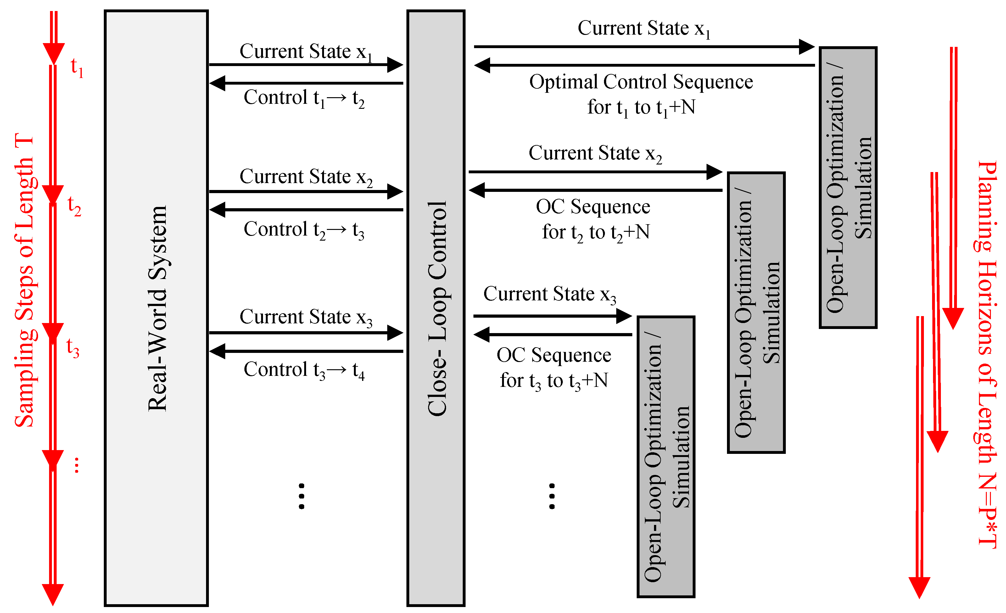
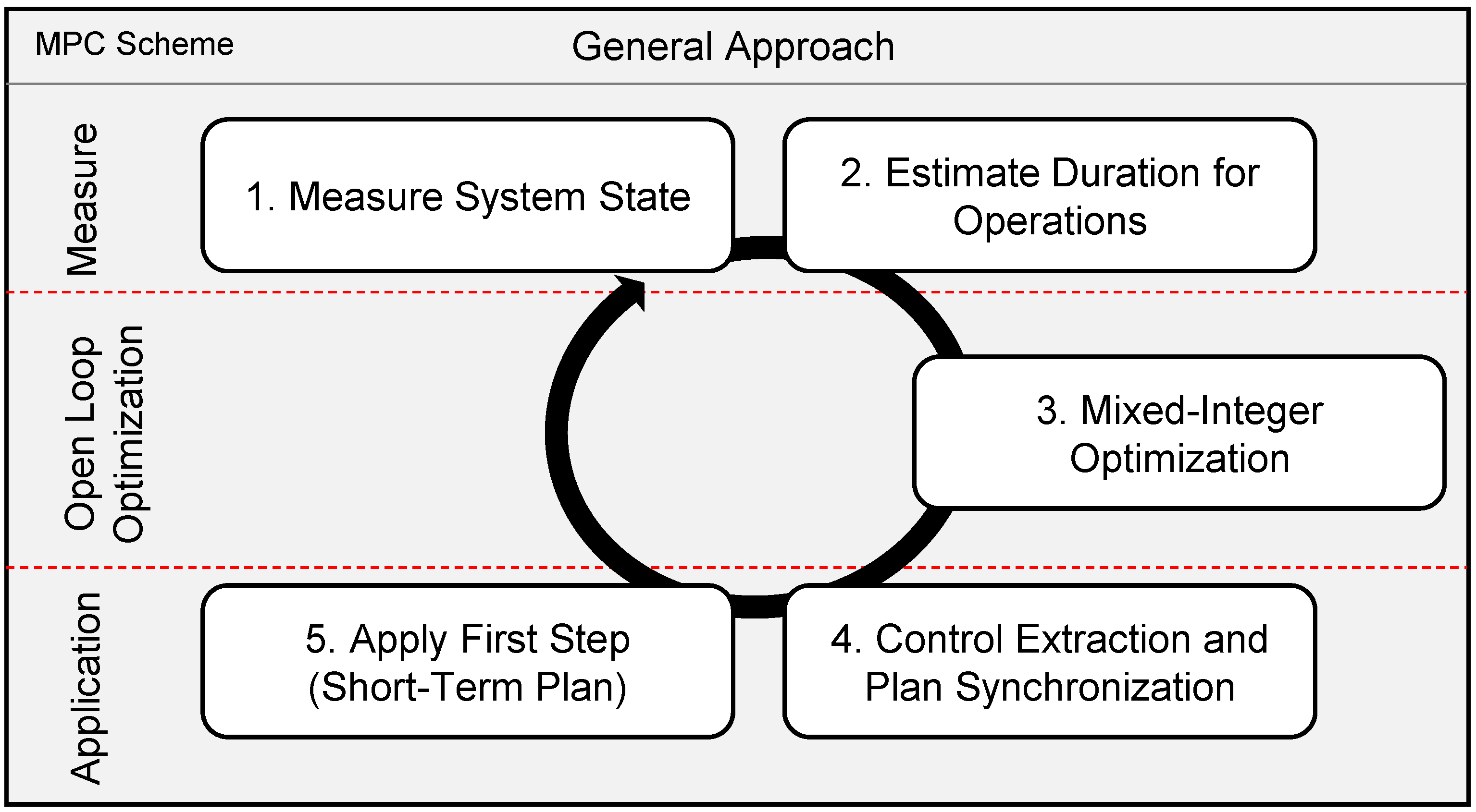
The MPC scheme applies a combination of two connected control loops, as depicted in Figure 2. The closed loop tethers to the controlled, real-world system. At distinct sampling instance $t_i$, the closed loop measures the current state of the real-world system denoted as state $x_i$. These sampling instances are distributed according to the sampling step size T. Afterward, the state gets forwarded to the open-loop optimization. This optimization uses so-called system models to estimate events and responses in the real-world system, and tries to obtain an optimal control sequence $u=\{u_1,u_2,\dots ,u_P\}$ for a simulated prediction horizon $N=P\times T$ with P denoting the number of planning periods of length T. The algorithm then passes this sequence back to the closed-loop control, which extracts the first control $u_1$ for the current sampling instance $t_i$ and applies it to the real-world system. As time progresses and reaches the next sampling instance $t_{i+1}$, the cycle starts over by measuring the current state of the system $x_{i+1}$ and thus, by evaluating the effects of the provided control.

The MPC scheme provides a viable baseline for the implementation of a decision-support system. It thereby implements the monitoring policy by selecting suitable values for the sampling step size, whereas the state defines all values that must be measured and monitored. In terms of the scheduling of offshore operations, the decision-support system should monitor deviations from a given plan/schedule. As the open loop already provides an optimized plan, deviations can be recognized quickly. As an intervention policy, this approach devises new schedules as recourse action, reacting to deviations by incorporating them into a new plan.

Where, for most common applications, the sampling step size T is only a few seconds or less, the adaptation of the MPC to the scheduling of offshore operations allows for substantially longer horizons. For this article, T is chosen as either 84 or 168 h, i.e., one week. The prediction horizon is generally varied between $N=168$ h (one week) and $N=540$ h (three weeks), as explained in more depth in Section 2.3. Due to the long horizons, each control subsumes a set of operations to be conducted within the corresponding week, thus representing a plan. Therefore, the control for the next sampling step size is considered a short-term plan, while the open loop’s optimal control sequence can be considered a mid- to long-term plan depending on the choice of P. As each plan consists of several operations, the realization of this plan is prone to failure. For the described scheduling problem, the primary source of dynamics stems from uncertainties in weather forecasts, and thus from uncertainties about the real duration of operations. In this context, a plan fails if an operation finishes too early or if it takes so long that follow-up operations cannot commence in time. Thus, plans may fail or finish before the next sampling instance. In the context of a decision-support system, it is a viable assumption that information on plan failures is available to the system. Moreover, as operations take a long time, it can be assumed that deviations from the plan can be anticipated early enough, to devise a new plan, i.e., to implement recourse actions. Therefore, the algorithm loosens the notion of sampling instances for this application. Instead of representing discrete time steps, a new sampling instance, and thus a new planning iteration, is initiated each time a plan finishes or fails. Nevertheless, every single plan aims to have a length equal to the sampling step size T for the closed loop or the corresponding prediction horizon N for the open loop.

Following the MPC scheme, the proposed approach consists of five steps, which apply to each sampling instance, as depicted in Figure 3. First, the current state of the real-world system is measured. This measurement includes updating the state of vessels, the number of built turbines, and weather forecasts. The second step estimates the duration of offshore operations for a prediction horizon N. Using this information, the third step creates a plan using a Mixed-Integer Linear Program during the open-loop optimization and returns this plan to the closed loop. The closed loop extracts a short-term plan of length T and calculates when the next sampling instance should occur if everything goes according to plan in step four. Finally, as the last step, the algorithm applies this plan to the real-world system.

For this article, we simulate the real-world system based on historical weather records. These records cover 50 years of hourly measurements of the wind speed and the wave height in Germany’s Northern Sea. As only measurements are available, the following evaluations simulate weather forecasts according to the stated accuracy given in Section 1.1. Consequently, the following subsections also include descriptions of how these forecasts are simulated and how the state is updated based on a simulated real-world system. For a real-world application, these steps can be omitted or simplified.

2.2. First Step: Representation of the State and Simulation of Weather Forecasts

The state comprises general information about the installation process and the current problem instance. The latter particularly subsumes information about the current date, the number, position, and loading state of vessels, the number of turbines to build, and the number of finished turbines. Additionally, the state contains general information, e.g., about costs or capacities required for the optimizer as given in Table 2 and information on the duration and restrictions of the considered operations. 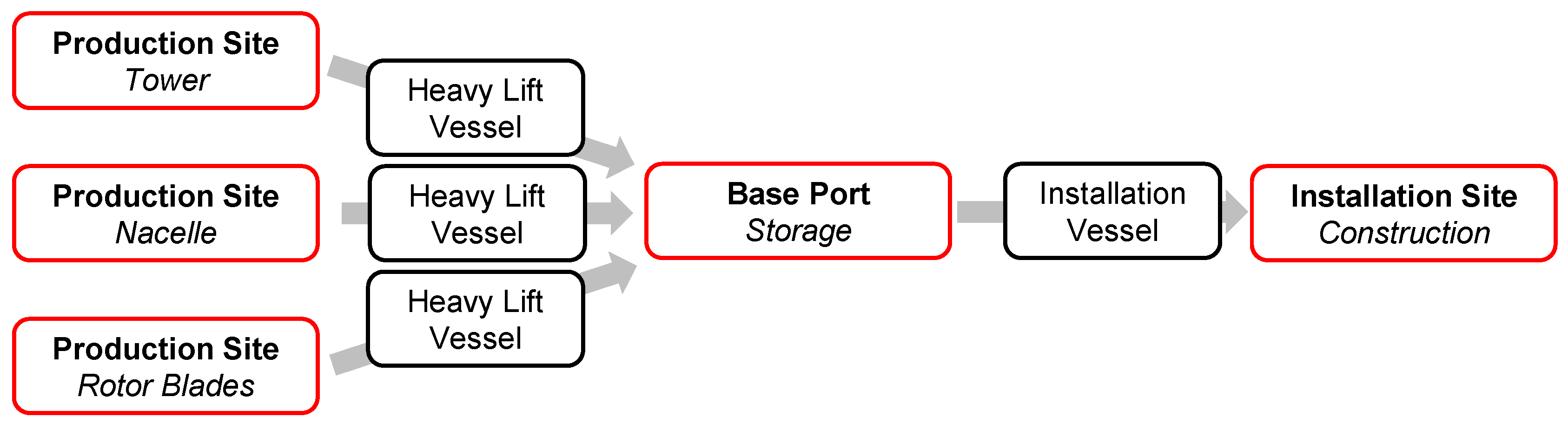As described in Section 1.1, the installation of a wind turbine occurs sequentially from bottom to top. This sequentiality allows simplifying the planning problem by applying aggregate operations, effectively reducing the number of considered operations from 12 to 4. While the basic operations given in Table 1 directly refer to tasks given in the process description, the aggregate operations, given in

Table 3. Aggregate operations used by the MILP model.

Operation	Base Duration (h)	Max. Wind (m/s)	Max. Wave (m)
Travel to Base Port	4	21	2.5
Travel to Construction Site	4	21	2.5
Load OWT	12	-	-
Install OWT	19	Depending on progress

, subsume sequences of basic operations. Therefore, the operation Load OWT is comprised of the loading of one tower, one nacelle, three blades, and one hub. The operation Install OWT subsumes the operations: position at foundation, jack-up, install tower, install nacelle, 3× install blade, install hub, and finally jack-down.

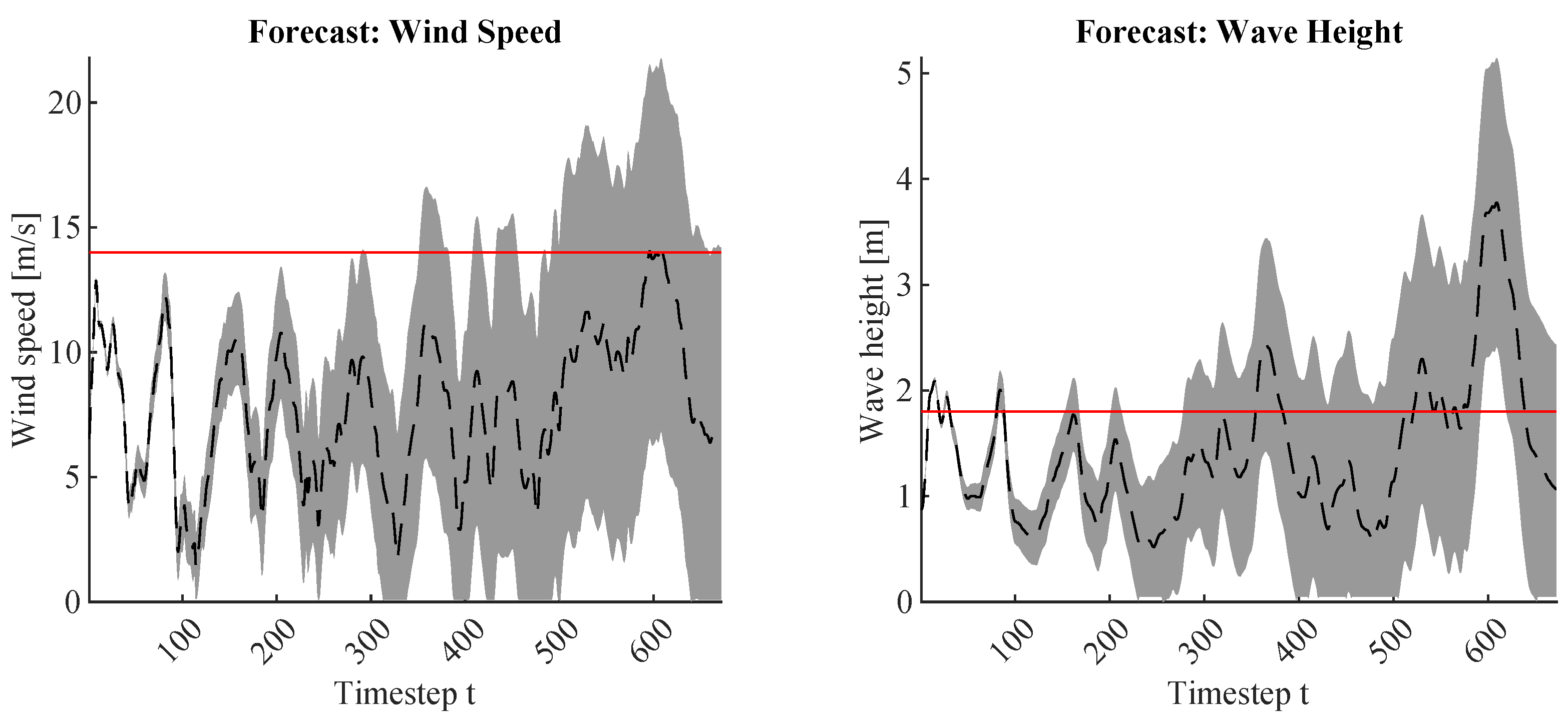
Finally, the state comprises the current weather forecast given as an interval of probable values for the wave height and wind speed for each hour within the prediction horizon N. As for this article, no real-world forecasts are available, forecasts are simulated from historical weather records as proposed in [9]. Compared to the original proposal, the forecast uncertainty has been adapted to provide more realistic assumptions. Therefore it is assumed that the uncertainty $\delta \left(t\right)$ starts at 0.0 for the current time instance, reaches 0.25 at 168 h into the future, and from there quickly increases to 0.65 at 336 h, 0.95 at 504 h, and from there increases even faster. The simulation first determines the average wind speed ${\mu }_s^{*}$ and wave height ${\mu }_h^{*}$ over the prediction horizon N. Afterward, for each time instance, the simulation obtains the measured values ${\mu }_s$ and ${\mu }_h$ from the historical recordings. Finally, the simulation acquires the forecast interval by multiplying the average values with the uncertainty and then adding/subtracting this value from the measurement: ${forecast}_s\left(t\right)={\mu }_s\pm ({\mu }_s^{*}·\delta \left(t\right))$ and ${forecast}_h\left(t\right)={\mu }_h\pm ({\mu }_h^{*}·\delta \left(t\right))$. Figure 4 shows the measurements as a black, dotted line and the generated intervals as gray areas for each hour of a forecasting horizon of three weeks. Additionally, the figure denotes the limits for a jack-up operation as a red line. The figure shows that the intervals strictly conform to the measured values in the beginning but begin to broaden quite quickly. As a result, larger proportions of the forecast intervals exceed the limits. This increase effectively reduces the probability of meeting these limits further into the forecast.

2.3. Second Step: Duration Estimation by Sliding Windows and Markov-Based Approaches

To handle weather dynamics with an hourly resolution and to cope with forecast uncertainties, the methodology discretizes weather forecasts in terms of an estimation of how long an operation takes if stated at a particular hour of the prediction horizon. These estimations are later used by the optimizer to obtain its plans. This approach avoids the use of stochastic or purely robust optimizations. A stochastic approach would require calculation of several samples, which, in combination with the embedded MILP, would lead to remarkably high computation times, unsuitable for a decision-support system. In contrast, a robust approach would always assume the worst possible case, which leads to high project costs and, for this application, to a high number of recourse actions as plans are considered to fail whenever a deviation between the planned and the real duration of operations occurs (cf. Section 2.1). This section first describes the original sliding-window approach proposed in [9]. Afterward, it introduces a new approach using Markov Chains, which eliminates the need for a user-based parametrization. The article presents a comparison of both approaches later in Section 3.1.

2.3.1. Discretization by Sliding Windows

The original methodology proposed a two-step approach. First, for each time instance within the prediction horizon and for each basic operation, the probability of having good-enough weather is calculated using the forecasts lower and upper bounds (gray area) and the corresponding limits indicated by the red line in Figure 4. Therefore, the approach assumes a uniform distribution for the interval. Consequently, it interprets the fraction of this interval, which lies below the limit, as the probability for having good-enough weather. In a second step, this approach estimates the duration of aggregate operations using a sliding window. This approach estimates the duration of aggregate operations as the sum over each basic operations’ duration plus the respective waiting times between those. It commences with the first basic operation at the requested starting time instance. It calculates the joint probability for a time window, corresponding to the length of the operation’s base duration, and compares this probability to a user-specified threshold $\omega$. If the joint probability is high enough, the window is accepted, and the algorithm proceeds to the next basic operation. This next operation is assumed to commence as soon as the previous one finishes. If the algorithm rejects the current window, i.e., the probability to successfully conduct the operation is too low, it shifts the window forward by one hour and reevaluates the new window. This shift represents the vessel waiting for one hour until it commences the operation. The algorithm performs this procedure for every aggregate operation and every possible starting hour within the prediction horizon.

While this approach provides a straightforward way to discretize the stochastic nature of weather forecasts, its estimation quality strongly depends on the selection of the parameter $\omega$. Therefore, this article proposes a more general way to estimate the duration of aggregate operations.

2.3.2. Discretization by Markov Chains

Since the weather data for wind speed and wave height come in a discrete form with an hourly resolution, the following approach discretizes the different basic operations and combines them in a directed graph. It represents each basic operation by a node, and each weighted edge represents the probability of transitioning to the adjacent node in the next time step. The goal is to estimate the average time needed to pass from the first to the last node in that graph. Since the probability of reaching the next node is only dependent on the weather forecast, the graph represents a discrete-time Markov Chain.

The used chain has three specific characteristics: First, each state points only on itself or to the following state with a combined probability of 1, since it is assumed that the operation was either successfully performed or not started at all. The second characteristic aims to render the problem easier to handle mathematically. This approach introduces helper states after each normal state. Therefore, a series of k helper states follow each normal state to represent the passing of time that is needed for that process to finish. The amount k of helper states conforms to the base duration of the respective operation minus one. The third characteristic describes that the final state is indeed final since it is not escapable. Let $P_{x,y}^n=P(X_{n+1}=y\mid X_n=x)$ be the probability of transitioning from state $x\in \mathbb{S}$ to $y\in \mathbb{S}$ with the state-space $\mathbb{S}$ at time step $t_n$. The state-space $\mathbb{S}$ thereby contains all the possible states from starting the turbine construction until the finished state, including all helper states in between. The stated characteristics from before are given as:

$$\begin{array}{cccccccc}\hfill P_{x,y}^n+P_{x,x}^n=1& & \forall n\in {\mathbb{N}}_0\hfill & & & & & \hfill \mathrm{if}y\mathrm{follows}x\\ \hfill P_{x,y}^n=1& & \forall n\in {\mathbb{N}}_0\hfill & & & & & \hfill \mathrm{if}x\mathrm{is}\mathrm{a}\mathrm{help}\mathrm{state}\\ \hfill P_{x,x}^n=1& & \forall n\in {\mathbb{N}}_0\hfill & & & & & \hfill \mathrm{if}x\mathrm{is}\mathrm{the}\mathrm{last}\mathrm{state}\end{array}$$

Since the weather and its forecast changes over time, most of the time $P_{x,y}^{n+1}\ne P_{x,y}^n$ which makes this Markov-Chain non-time-homogeneous and results in a time-dependent transition matrix $P^n$ with the entries $P_{x,y}^n$.

Writing the states as a vector s with a length equal to the number of states with its binary entries indicating which state s is represented, it is possible to apply the transition matrices $P^0,\dots ,P^n$ on the initial state to calculate the probabilities of the states at time step $t_n$. Figure 5 displays an example transition matrix. Let $s_0=[1,0,\dots ,0]$ indicate the initial state, then the last entry of $s_i=s_0{\prod }_{i=0}^n{P}^i$ represents the probability of being in the final state at time step $t_n$. This approach uses a weighted sum $d={\sum }_{i=1}^{\infty }i·p_i$ with $p_i=s_i\left(q\right)-s_{i-1}\left(q\right)$ and q equal to the number of all states to estimate the average time d needed to reach the final state. Since it is possible that $s_i\left(q\right)<1$ $\forall i\in {\mathbb{N}}_0$, the sum does not need to converge. This particularly happens, if an operation cannot finish during the forecast period due to high uncertainties or bad weather. For numerical purposes, this approach caps the sum after $s_i\left(q\right)>0.9973$, which correlates with a standard deviation of $3\sigma$ in a normal distribution.

The Markov-Chain approach uses the presented concepts in combination with the limits on weather restrictions provided in Table 1 to estimate the duration of aggregate operations. Therefore, it compares the limits for each operation with the minimum $l_{i,j,r}$, and maximum $u_{i,j,r}$ of the forecast for every time step $t_i,\dots ,t_{i+d-1}$ to calculate the probability that the operation could finish successfully if started at time step $t_i$. Therefore, d denotes the specified base duration of that operation (c.f. Table 1), $j\in \{0,\dots ,d-1\}$ and r indicates the respective weather restriction. The minimum and maximum value serve as $3\sigma$-boundaries for a normal distribution $\mathcal{N}(\mu ,\sigma )$ with the mean $\mu =(u_{i,j,r}+l_{i,j,r})/2$ and the standard deviation $\sigma =((u_{i,j,r}-l_{i,j,r})/2)/3$ to estimate the success probability for an operation at a certain time step. This way, 99.73% of the time, the actual value will be inside the interval given by the minimum and maximum. This approach then uses the value of the cumulative distribution function $\mathsf{\Phi }(x,\mu ,\sigma )$ of the normal distribution $\mathcal{N}(\mu ,\sigma )$ with x as the operation’s limit as the probability for that time instance. Finally, it selects the overall probability for the operation at the specified time step as the minimum probability across all requirements r and time steps $t_i,\dots ,t_{i+d-1}$. The approach chooses the minimum, as all requirements must be fulfilled to conduct the operation successfully. As a result, the lowest probability reflects the overall success chance.

2.4. Third Step: MILP Formulation for the Incremental Scheduling of Offshore Operations

After preprocessing the weather forecasts to obtain an estimation of the duration for each aggregate operation at each time instance, the open loop calculates a plan for the prediction horizon N. As can be seen from the state of the art, several possible formulations and approaches exist for this task. Following the assumptions given in Section 2.1, i.e., that plans cover about a week or even more and that deviations can be anticipated comparably early due to the long duration of operations, this article proposes to exploit these extended time frames and to strive for exact mathematical solutions. Consequently, this section proposes a Mixed-Integer Linear Program for the scheduling. As this article considers multiple vessels with equal capabilities, a Flexible JSSP formulation is selected. According to the classification in Section 1.3, there exist three basic formulations: a precedence-based formulation, a sequence-based formulation, or a time-indexed formulation. Whereas time-indexed formulations are the slowest to compute, they provide several advantages over the other formulations for this application. On the one hand, it is possible to directly make use of varying processing times, i.e., to directly include the estimated duration for aggregate operations. For sequence-based formulations, this is hard to achieve due to their abstract representation of time. On the other hand, a time-indexed formulation can easily be parameterized to obtain plans for a predetermined time frame, i.e., the prediction horizon N. This is very hard to formulate for precedence-based models. Such models index the scheduling problem over the number of operations, and thus, always must schedule all operations. For the proposed incremental approach, this will be impossible in most of the cases, as forecasts only remain reliable for comparably short forecast horizons. Therefore, the optimizer might not be able to schedule all operations within the prediction horizon, rendering the problem infeasible. For time-indexed models, the problem can be reformulated to instruct the optimizer to schedule as many operations as possible within the prediction horizon, favoring incremental approaches.

As stated before, the Mixed-Integer formulation used in this article is an extension to the one used in [9]. This article extends the formulation to handle multiple installation vessels and by constraints, which limit the number of available loading bays in the base port. Moreover, it presents a modification to the overall formulation, which includes so-called penalty terms. These terms, e.g., provide benefits for finishing an operation early, to reduce the model’s symmetry, and to speed up the optimization. Table 2 in Section 1.6 provides an overview of the relevant model parameters and variables.

The model aims to minimize the cost function J given in Equation (1) under consideration of the constraints given in Equations (2)–(15). The MILP optimizes a plan for the prediction horizon N determined by the sampling step size T and the previously defined number of planning periods P as $N=P\ast T$ (c.f. Section 2.1. Cost function J sums the cost for vessels being offshore, fuel cost for traveling between the site and base port, and hourly costs for port operations. Therefore, it sums each occurrence of such an operation and, respectively, every hour a vessel is offshore and multiplies these sums with the associated costs (first line of Equation (1)). It is advised to choose different costs for each vessel to reduce model symmetry. Even if the same vessels are applied, a small offset should be added to render some vessels slightly less favorable to the optimizer, e.g., by adding just 0.1 to the costs of vessel two, 0.2 to vessel three, and so forth. This offset guarantees that the plans are not interchangeable between vessels. Moreover, small offsets only have a marginal impact on the overall cost. 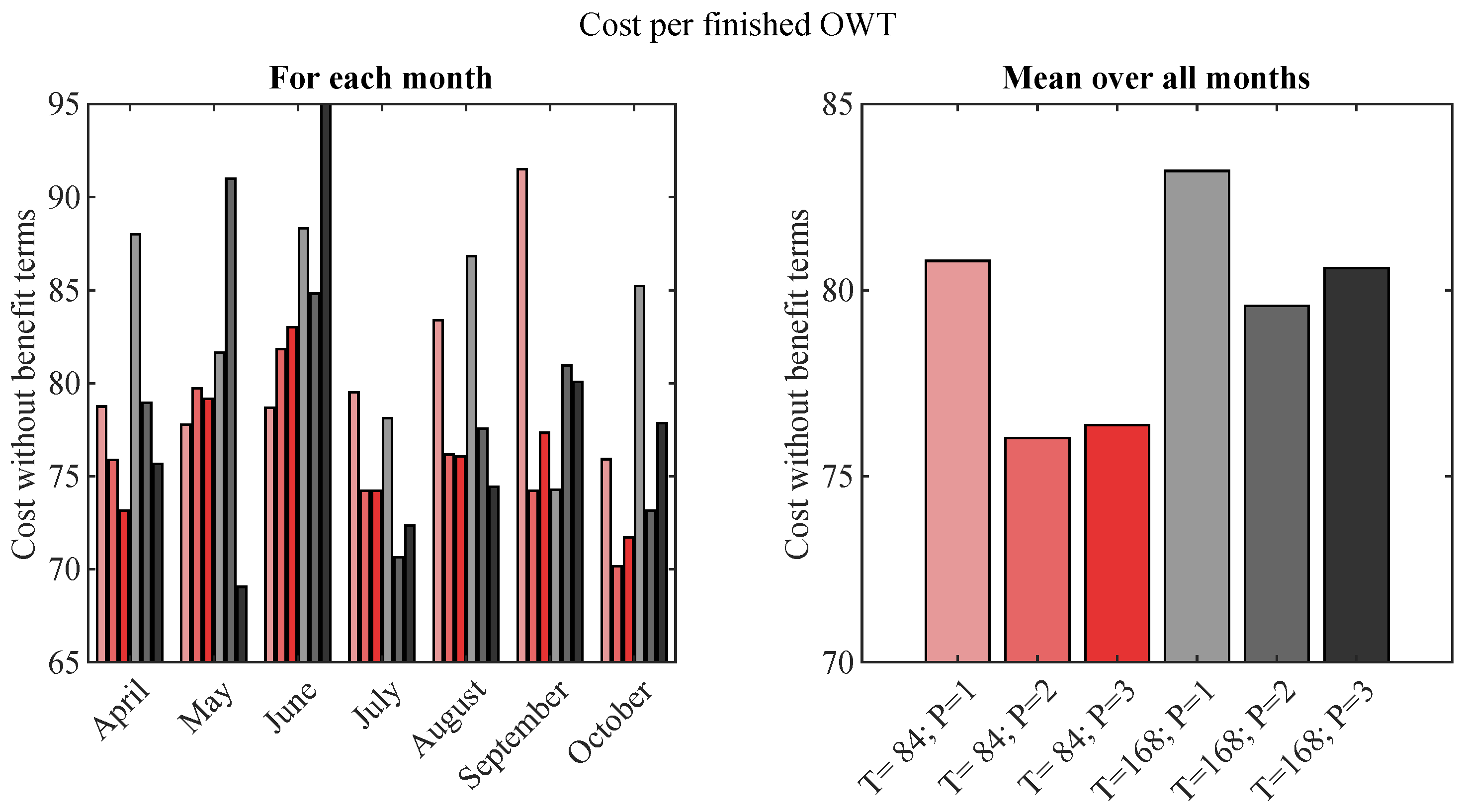Additionally, the cost function applies three different penalty terms (second line of Equation (1)). The first term assigns a bonus $B^{owt}$ (negative cost) for each finished OWT. The other two terms assign an increasing bonus $B^{early}$ the earlier an operation finishes during the prediction horizon. Therefore, the cost function first normalizes the finish time of an operation over N to be between 0 and 1 and then inverts this value by subtracting one from it. Finally, this value is multiplied with $B^{early}$ and added to the penalty term. For non-installation operations, this bonus is scaled down to prevent the optimizer from favoring shorter operations over longer ones, i.e., to prevent it from fully loading the vessel to get this bonus when it would be possible to finish installation tasks instead. These two penalty terms aim to reduce the symmetry of the model, as described later.

$$\begin{array}{}\left(1\right)& \hfill J& ={\displaystyle \sum _{v=1}^V}({\displaystyle \sum _{k=1}^N}(Y_{v,k}^{loc})·C_v^o+{\displaystyle \sum _{k=1}^N}(Y_{v,k}^{atBay})·C_v^p+{\displaystyle \sum _{k=1}^N}(Y_{v,k}^{toSite})·C_v^m+{\displaystyle \sum _{k=1}^N}(Y_{v,k}^{toPort})·C_v^m)\hfill & & -{\displaystyle \sum _{v=1}^V}({\displaystyle \sum _{k=1}^N}(Y_{v,k}^{owt}·B^{owt})+{\displaystyle \sum _{k=1}^N}(\frac{X_{v,k}^{fOwt}}{N}-1)·-B^{early}+{\displaystyle \sum _{k=1}^N}(\frac{X_{v,k}^{fOp}}{N}-1)·(-0.2·B^{early}))\hfill \end{array}$$

As the model uses an hourly, time-indexed formulation over several vessels, all decision and support variables have the dimensions of $V\times N$ with V being the number of applied installation vessels and N representing the prediction horizon in hours. The extended model uses four binary decision variables $Y_{v,k}^{owt}$, $Y_{v,k}^{load}$, $Y_{v,k}^{toPort}$, $Y_{v,k}^{toSite}$ instead of only one in the original model. These denote if a specific vessel $v\in {\mathbb{N}}^{+}$ starts an aggregate operation of the given type (install OWT, load components, move to port, move to site) at a given time instance $k\in {\mathbb{N}}^{+}$. Whereas these variables could be summarized as a single variable that is indexed over the operation, the model and the resulting code remain easier readable and maintainable by using distinct variables. Additionally, the model uses a total of six support variables, which directly depend on the four decision variables. These variables generally denote ongoing events. For example, if an installation is started, the MILP notes this as part of the decision variable $Y_{v,k}^{owt}$. Additionally, it denotes the ongoing installation process using the dependent support variable $Y_{v,k}^{busy}$. Moreover, this support variable records the duration of all ongoing operations, i.e., loading, movement and installation operations.

The variables $Y_{v,k}^{loc}$, and $X_{v,k}^{cap}$ record the position and amount of currently loaded components for each vessel at each time instance. Therefore, constraints (2) and (4) use a very similar formulation. For example, these constraints denote the capacity as equal to the last time step plus one for a started loading operation and minus one for a commenced installation operation. Additionally, they constrain the capacity by a specified maximum capacity $CAP$ by constraint (3). The location is formulated similarly but refers to movement operations instead. As both constraints rely on the previous time instance, the MILP contains additional constraints for the first time instance in a similar fashion. Instead of referring to the previous instance, these constraints use an initial value provided to the optimizer instead.

$$\begin{array}{cccc}{X}_{v,k}^{cap}=X_{v,k-1}^{cap}-Y_{v,k}^{owt}+Y_{v,k}^{load}\hfill & & & \hfill \forall k\in \{2\dots N\};\forall v\in \{1\dots V\}\end{array}$$

(2)

$$\begin{array}{cccc}{X}_{v,k}^{cap}\le CAP\hfill & & & \hfill \forall k\in \{1\dots N\};\forall v\in \{1\dots V\}\end{array}$$

(3)

$$\begin{array}{cccc}{Y}_{v,k}^{loc}=Y_{v,k-1}^{loc}-Y_{v,k}^{toPort}+Y_{v,k}^{toSite}\hfill & & & \hfill \forall k\in \{2\dots N\};\forall v\in \{1\dots V\}\end{array}$$

(4)

The support variables $Y_{v,k}^{busy}$, and $Y_{v,k}^{atBay}$ track if a specific vessel is generally busy and, additionally, if it is currently performing a loading operation at the base port. Constraints (5)–(9) record these durations. Constraints (5)–(8) thereby mark the corresponding entries in $Y_{v,t}^{busy}$ for $t=k+1$ to $(k+D_{o,k}-1)$ for the corresponding vessel v and the scheduled operation o. This indicates that no other operation can be scheduled during this period (c.f. Constraint (10)). As can be seen from this formulation, the constraints do not mark the time instance k itself, as this is already marked in the corresponding decision variables. Consequently, these constraints also subtract one hour from the duration. In contrast, $Y_{v,k}^{atBay}$ denotes the full duration from k to $k+D_{o,k}$.

$$\begin{array}{cccc}{\displaystyle \sum _{t=k+1}^{k-1+D_{1,k}}}{Y}_{v,t}^{busy}\ge Y_{v,k}^{owt}·(D_{1,k}-1)\hfill & & & \hfill \forall k\in \{1\dots N\};\forall v\in \{1\dots V\}\end{array}$$

(5)

$$\begin{array}{cccc}{\displaystyle \sum _{t=k+1}^{k-1+D_{2,k}}}{Y}_{v,t}^{busy}\ge Y_{v,k}^{toPort}·(D_{2,k}-1)\hfill & & & \hfill \forall k\in \{1\dots N\};\forall v\in \{1\dots V\}\end{array}$$

(6)

$$\begin{array}{cccc}{\displaystyle \sum _{t=k+1}^{k-1+D_{3,k}}}{Y}_{v,t}^{busy}\ge Y_{v,k}^{toSite}·(D_{3,k}-1)\hfill & & & \hfill \forall k\in \{1\dots N\};\forall v\in \{1\dots V\}\end{array}$$

(7)

$$\begin{array}{cccc}{\displaystyle \sum _{t=k+1}^{k-1+D_{4,k}}}{Y}_{v,t}^{busy}\ge Y_{v,k}^{load}·(D_{4,k}-1)\hfill & & & \hfill \forall k\in \{1\dots N\};\forall v\in \{1\dots V\}\end{array}$$

(8)

$$\begin{array}{cccc}{\displaystyle \sum _{t=k}^{k-1+D_{4,k}}}{Y}_{v,t}^{atBay}\ge Y_{v,k}^{load}·D_{4,k}\hfill & & & \hfill \forall k\in \{1\dots N\};\forall v\in \{1\dots V\}\end{array}$$

(9)

Constraint (10) exploits this behavior and uses the resulting support variable $Y^{busy}$ and the decision variables to ensure that each vessel is only involved in a single operation at a time.

$$\begin{array}{cccc}{Y}_{v,k}^{owt}+Y_{v,k}^{load}+Y_{v,k}^{toPort}+Y_{v,k}^{toSite}+Y_{v,k}^{busy}=1\hfill & & & \hfill \forall k\in \{1\dots N\};\forall v\in \{1\dots V\}\end{array}$$

(10)

Constraint (11) limits the number of available loading bays to a specified value $BAYS$. This constraint uses the parameter ${INUSE}_k^{bays}$, which denotes how many loading bays are in use by previous schedules at each time instance k.

$$\begin{array}{cccc}{\displaystyle \sum _{v=1}^V}{Y}_{v,k}^{atBay}+{INUSE}_k^{bays}\le BAYS\hfill & & & \hfill \forall k\in \{1\dots N\}\end{array}$$

(11)

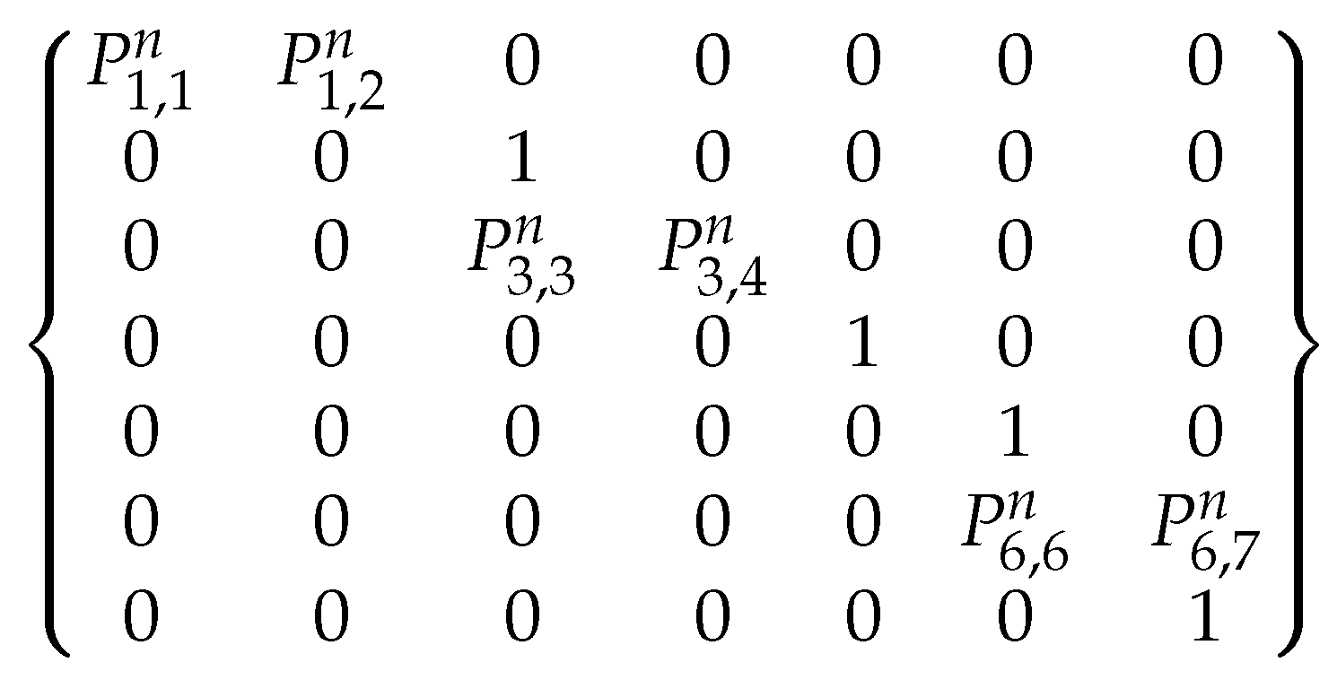
Constraint (12) ensures that the optimizer only schedules installation activities if they can be finished within the prediction horizon N. To record the duration, the model uses a provided matrix of expected durations $D_{o,k}$. This matrix denotes the duration of an operation o if it is started at a time instance k. Therefore, the index o refers to the aggregate operations install owt = 1, move to port = 2, move to site = 3 and load components = 4. This matrix is calculated outside of the optimizer, as described before, in Section 2.3.

$$\begin{array}{cccc}{Y}_{v,k}^{owt}\le max(0,(N-k)-(D_{1,k}-1))\hfill & & & \hfill \forall k\in \{1\dots N\};\forall v\in \{1\dots V\}\end{array}$$

(12)

The last two support variables reduce the symmetry of the formulation by recording the finishing time of operations. Symmetry occurs when two or more alternative solutions result in the same value for the cost function. For example, if an operation takes the same amount of time when it starts at hour 1 or hour 2, and this decision has no effect on the rest of the solution, a symmetrical situation occurs. By adding penalty terms to the cost function, it is possible to assign small benefits to operations that finish earlier in the process and, thus, to remove this symmetry. Therefore these variables record the expected finish times of installation operations $X_{v,k}^{fOwt}$, and of all other operations $X_{v,k}^{fOp}$ using constraints (13) and (14).

$$\begin{array}{cccc}{X}_{v,k}^{fOwt}=Y_{v,k}^{owt}·(k+D_{1,k}-1)\hfill & & & \hfill \forall k\in \{1\dots N\};\forall v\in \{1\dots V\}\end{array}$$

(13)

$$\begin{array}{}& X_{v,k}^{fOp}=Y_{v,k}^{toPort}·(k+D_{2,k}-1)\hfill & & \left(14\right)& +Y_{v,k}^{toSite}·(k+D_{3,k}-1)+Y_{v,k}^{load}·(k+D_{4,k}-1)\hfill & & \hfill \forall k\in \{1\dots N\};\forall v\in \{1\dots V\}\end{array}$$

The final constraint (15) is required to prevent the optimizer from scheduling vessels that are not currently available. As specified as part of the general methodology (Section 2.1), the MPC-based algorithm applied an incremental planning and scheduling approach. If applying several vessels, the algorithm calculates a joint plan for all of them. Nevertheless, the vessels’ single sub-plans may end or fail at different times. For example, if the plan covers two vessels and one finishes at hour 90 while the other’s plan ends at hour 100, a new planning iteration will start at hour 90. As a result, the second vessel cannot be assigned for the first 10 h of the new planning iteration. Thus, the optimizer will not issue new operations to a vessel v until the respective delay, provided as ${START}_v$, is reached. This ensures that the newly derived plan will not override unfinished, but already scheduled operations.

$$\begin{array}{cccc}{Y}_{v,k}^{busy}\le max(0,k-{START}_v)\hfill & & & \hfill \forall k\in \{1\dots N\};\forall v\in \{1\dots V\}\end{array}$$

(15)

2.5. Fourth Step: Control Extraction and Plan Synchronization

Compared to the original approach, this article only proposes some minor changes to the extraction of the next short-term plan. The algorithm extracts a plan for each involved vessel by copying all scheduled operations, which will finish within the sampling step size T. As these plans can each have a different length, the scenario description denotes the estimated next sampling instance $t_{i+1}$ as the end of the shortest plan. The algorithm updates the state with an indicator for each vessel, for how many hours into the new planning period it is still scheduled, i.e., when the vessel’s plan will end in relation to the shortest devised plan. An example of this is already given in Section 2.4 for the description of constraint (15). The algorithm performs the same for port-side resources, i.e., for the loading bays.

2.6. Fifth Step: Apply Short-Term Plan and Simulation of the Real-World System

In each iteration’s final step, the algorithm forwards the extracted short-term plans to the real-world system for execution. If all operations can be applied as planned, the closed loop uses the previously determined values for the next planning iteration (sampling instance and the remaining length of vessel plans) to initiate the next planning period. Nevertheless, as this methodology is designed to act as online decision support, it can update these parameters in case of plan failures. If the decision-support system is notified of an anticipated plan failure, it measures the current state of the real-world system. As described in Section 2.2, this includes an update of each vessels’ state (position, loaded components, remaining plan length, etc.), the overall project’s state in terms of built turbines, and of the weather forecasts.

The simulation of the real-world system uses the already mentioned historical weather records as described in the original approach. Therefore, it compares the duration of each scheduled operation to its real duration. It thereby computes this real duration in the same way as the expected duration, but without any forecast uncertainty, i.e., by selecting the lower and upper bounds both according to the actual historical recording. This way, the forecast uncertainty is removed, and it is possible to calculate if an operation can take place or not. An operation is then considered to fail in two cases: Either if the real duration is shorter than the expected one, which would induce additional waiting times and costs, or if the real operation takes longer than expected and thereby leads to the vessel missing follow-up operations. The simulation performs this comparison for each vessel separately, determining which plan ends at which time instance. Afterward, the state is updated as described before, and the simulation time advances to either the next pre-calculated sampling instance or to the time instance for which the earliest plan failure occurs. As described earlier, the algorithm blocks vessels with remaining schedules for an appropriate duration using the MILPs parameter ${START}_v$ in Constraint (15).

3. Results

This section aims to provide an extensive evaluation of different aspects concerning the proposed methodology and its extensions. Therefore, it first presents a comparison between the two proposed methods for the estimation of the duration of offshore operations, i.e., the sliding-window approach and the approach using Markov Chains. Afterward, this section presents different sets of numerical simulations to evaluate the effect of loading bay restrictions and the overall extended MPC-based approach. The first set aimed to evaluate the impact of loading bay restrictions without the influence of weather forecast uncertainties. Therefore, only the MILP described in Section 2.4 was used to generate non-incremental, optimal plans. The second set of simulations aim to determine a suitable configuration for the prediction horizon and sampling step size used by the MPC-based approach. Therefore, a single vessel was simulated using a sampling step size T of one week and half-a week, and prediction horizons of respectively one, two, and three times T to evaluate the quality of the generated plans. The third set of simulations aims to evaluate the response time of this approach, as response times constitute a critical factor for decision-support systems.

In all cases, the algorithm and the MILP are implemented in MATLAB r2018b using a problem-based formulation, while the optimization was executed using CPLEX 12.9 on an ordinary quad-core office computer (i7-3770K, 8GB RAM) using the opportunistic search mode. For solving larger instances of the problem, the optimizer aborts if the solution quality stagnated. Therefore, the maximum optimization time for each run was set to three hours. After a run finished, another run was started, again running for a maximum of three hours using the best previous encumberment as its initial solution. If successive runs were unable to find another encumberment, the algorithm selects the best previous encumberment as the final solution. These restarts were conducted, as CPLEX applies a cut and branch strategy. Therefore, experiments showed, CPLEX makes most of the progress for larger scenarios during the initial cutting stage and the first hours of the branching stage, often resulting in an optimal or near-optimal solution with only a few repetitions. Moreover, the optimizer behaves differently for different initial solutions, which makes it useful to try again with another solution.

3.1. Comparison of Approaches for the Estimation of Operation Durations

This section aims to evaluate the differences between the two approaches for the discretization of forecast uncertainties described in Section 2.3. Therefore, this experiment applies both approaches to the months from April 2000 until October 2000. This procedure was repeated for different estimation horizons of one to four weeks. For the sliding-window approach, the parameter $\omega$ was optimized manually in steps of 0.05 for each month, so that the estimation error was as small as possible. It is to mention that this is only possible when applied to historical information. For real-world applications, a best-guess must be applied.

Table 4. Comparison of the sliding window and the Markov approach.

2000	Apr.	May	Jun.	Jul.	Aug.	Sep.	Oct.	Mean
Act. dur. Min	19	19	19	19	19	19	19	19.00
Act. dur. Mean	23	23	28	30	20	26	31	25.86
Act. dur. Max	69	81	85	101	41	74	130	83.00
Standard Deviation: Sliding Window in hours
1 Week	0.22	1.77	1.41	2.21	0.00	0.57	0.86	1.01
2 Weeks	2.16	1.25	3.29	3.67	0.00	3.11	2.10	2.23
3 Weeks	2.10	3.07	20.81	20.15	0.55	10.18	15.93	10.40
4 Weeks	35.82	77.29	31.79	17.45	1.79	94.42	335.87	84.92
Standard Deviation: Markov in hours
1 Week	0.26	0.67	2.56	0.58	0.00	1.47	0.77	0.90
2 Weeks	1.07	0.53	1.99	2.28	0.08	2.86	6.30	2.16
3 Weeks	1.14	0.95	4.06	12.73	0.29	5.02	5.59	4.25
4 Weeks	1.08	3.07	6.78	11.02	1.26	5.26	77.85	15.19

summarizes the results of the comparison. Therefore, it first states the minimal, mean, and maximal actual duration of the operation Install OWT for each month as a reference. The actual values result from applying the Markov approach to the historical weather records without using forecast uncertainties, as described earlier in Section 2.6. Afterward, the table lists the corresponding approaches’ estimation errors for prediction horizons of one to four weeks. The table provides the estimation error as the standard deviation between the estimation and the actual value over the corresponding period for each month. The final column Mean always depicts the mean value of the corresponding row. Therefore, all these horizons start at the first of the current month until the end of the noted week.

As expected, the error increases with an increasing horizon. For one week, the average estimation error is approximately one hour for both approaches, increasing to 84.92 h for the sliding-window approach and 15.19 h for the Markov approach at four weeks. In general, for one or two weeks, both approaches perform similarly well, but for longer horizons, the Markov approach outperforms the sliding-window approach by far. Figure 6 shows an example of the estimations for weeks 2 and 3 of the April dataset. Comparing both approaches shows that the Markov-Chain approach results in smoother estimations but tends to underestimate the real duration slightly. Nevertheless, its estimation follows the general shape of the actual duration quite closely. In contrast, the sliding-window approach tends to overestimate. In conclusion, the Markov approach generally performs better and, additionally, is not dependent on an optimal parametrization. Therefore, the remaining experiments provided in this article use the Markov approach for the discretization of weather uncertainties.

3.2. Evaluation of the Influence of Limited Resources Without Forecast Uncertainties

This experiment aims to provide insights into the relationship between the number of vessels and loading bays under different weather conditions. For the latter, the evaluation focusses on June, August, and October 2000. As given in Table 4, August provides close to perfect weather conditions, while October has the worst still suitable weather conditions in 2000. June was selected as it provides a comparably moderate mix of good and bad conditions. For the assessment of the impact of loading bay restrictions, this evaluation uses different combinations of vessels and bays over a time frame of three weeks. Therefore, it covers different ratios between vessels and bays. The evaluation also includes some experiments with equal ratios to ensure that this ratio provides a suitable indicator. The parameter selection for V and $BAYS$ thereby followed a factorial design with the aim, to achieve an as broad as possible coverage of ratios between these two. All the optimizations use the MILP formulation in Section 2.4, without the inclusion of weather uncertainties.

Table 5. Results for different combinations of vessels and loading bays.

Scenario			June			August			October
Bays	Vessels	Bays/Vessels	OWTs Finished	Per Vessel	Bay Use	OWTs Finished	Per Vessel	Bay Use	OWTs Finished	Per Vessel	Bay Use
1	1	1.00	14	14.00	0.31	14	14.00	0.31	12	12.00	0.28
2	2	1.00	28	14.00	0.31	28	14.00	0.31	24	12.00	0.28
3	3	1.00	42	14.00	0.31	42	14.00	0.31	36	12.00	0.28
4	4	1.00	56	14.00	0.31	56	14.00	0.31	48	12.00	0.28
3	4	0.75	51	12.75	0.37	56	14.00	0.41	41	10.25	0.32
1	2	0.50	24	12.00	0.52	28	14.00	0.61	20	10.00	0.46
2	4	0.50	48	12.00	0.52	56	14.00	0.61	40	10.00	0.46
1	3	0.33	33	11.00	0.72	35	11.67	0.76	26	8.67	0.60
1	4	0.25	33	8.25	0.72	35	8.75	0.76	26	6.50	0.60
1	5	0.20	33	6.60	0.72	35	7.00	0.76	26	5.20	0.60
1	10	0.10	33	3.30	0.72	35	3.50	0.76	26	2.60	0.60

summarizes the results.

Figure 7 depicts the number of finished turbines per vessel (a) and the normalized bay use (b) for different ratios between bays and vessels for each of the evaluated months. The figure shows that the general shape for each month is very similar. Therefore, a high ratio results in a high number of finished turbines and a low bay use. In contrast, for ratios of less than 0.33, the use reaches a plateau. Deploying more than three vessels for a single bay does not increase the number of finished turbines in any of the evaluated months. Furthermore, the figure shows a strong influence of the weather conditions on the overall number of finished turbines and the bay use. While the deployment of only a single vessel per bay results in a comparably equal number of finished turbines per vessel, it declines faster for worse conditions. The results show that the number of finished turbines per vessel decreases by 7.5% for a ratio of 0.75 if comparing the average number of finished turbines to the best case (ratio of 1). This loss increases to 10% for a ratio of 0.5 (two vessels, one bay) and drastically increases to 21.67% for a ratio of 0.33 (three vessels one bay). As stated before, after this point, a steady, linear decrease can be observed, as the number of finished turbines stagnates.

In conclusion, these results show that the efficiency of deployed vessels and the use of bays strongly depends on available weather windows. The results indicate that three vessels per bay constitute the maximum sensible amount if aiming for high use, at the cost of an average of 21.67% efficiency. The deployment of two vessels per bay (ratio of 0.5) shows a good trade-off in terms of efficiency and use.

3.3. Evaluation of the Influence of the Number of Planning Periods on the Incremental Approach

This evaluation focuses on several combinations of the parameters P and T using the presented MPC-based approach to determine good settings for the sampling step size and the number of planning periods. Therefore, it simulates a single vessel with a project starting date for each month between April and October 2000 to cover several different compositions of weather conditions. This evaluation uses the number of wind turbines finished within a four weeks horizon, and the number of plans, required to cover these four weeks, to compare the results. The experiments use a time frame of four weeks to cover enough time but to prevent overlaps between the months. Therefore, the number of finished turbines indicates an efficient plan, while a low number of plans indicates that few plan failures occur, which always causes recourse actions.

Table 6. MPC results for different T and P.

	OWT	Plans	OWT	Plans	OWT	Plans	OWT	Plans	OWT	Plans	OWT	Plans
T/P	84/1		84/2		84/3		168/1		168/2		168/3
Apr.	16	10	17	8	19	8	16	5	17	4	18	4
May	17	10	18	8	18	8	17	5	17	5	18	4
Jun.	13	11	17	8	17	9	16	5	16	5	16	5
Jul.	14	10	18	8	17	8	16	6	17	4	17	5
Aug.	18	10	19	8	18	8	18	5	18	4	18	4
Sep.	12	10	18	8	18	8	18	5	17	5	16	5
Oct.	12	9	13	9	14	9	13	6	13	6	13	6
Sum	102	70	120	57	121	58	114	37	115	33	116	33

summarizes the results of these experiments. These experiments again follow a factorial design: T is either chosen as 84 h (half-a week) or 168 h (one week), and P is selected as either 1, 2, or 3 times the sampling step size. The latter follows previous results, which demonstrate that longer prediction horizons do not increase the solution quality [9]. The values for P have been chosen for an easier interpretation and result in prediction horizons of one, two, and three weeks for the case of $T=168$ h. The same values apply for the case of $T=84$ h to retain comparability, resulting in prediction horizons of half-a week, one week, and one-and-a-half week. It must be noted that P does not necessarily need to be an integer as long as it is guaranteed that T and N are integers. The approach uses the latter for indexing and thus requires integer values. As can be seen from the results, a prediction horizon of 84 h (T = 84, P = 1) results in comparably inefficient plans. Thus, this experiment does not consider smaller sampling step sizes. In contrast, the calculation time for each iteration increases drastically with an increasing prediction horizon. The optimizer is not capable of obtaining optimal solutions for a prediction horizon of three weeks (T = 168, P = 3), and all simulations finish due to stagnation. While this does not necessarily mean that the solution is sub-optimal, the optimizer could not prove its optimality in time. For this reason, this experiment excludes longer sampling step sizes as well.

As can be seen from Table 6, selecting $P=1$ resulted in the worst plans for each sampling step size, generally resulting in more plans needed. Therefore, for four weeks, a minimum of eight ($T=84$) or four ($T=168$) plans would be the minimum for the respective sampling step size. Additionally, selecting a single planning period resulted in less built OWTs for both settings. This decrease shows that the application of an MPC scheme is advantageous for such planning problems, as the longer prediction horizons in the open loop result in better solutions than just relying on a simple rolling horizon planning. Comparing the remaining combinations for $T=84$ and $T=168$ shows a higher number of finished OWTs for the shorter sampling step size. Moreover, shorter sampling step sizes required fewer additional plans. The influence of forecast uncertainties can explain this decrease. For shorter plans, these uncertainties are less likely to cause plan failures or wrong estimations. Finally, comparing the results for $P=2$ and $P=3$ for the shorter sampling step size, it can be observed that $P=2$ results in one less finished turbine, while also requiring one less plan if comparing all simulated months. Figure 8 shows the cost per finished turbine per month (left) and the average across all simulated months for each combination of T and P (right). Therefore, only the cost part of the cost function in Equation (1) was recalculated for all operations, which finished within the first four weeks of the generated plans, ignoring the penalty terms. As can be seen, the average cost of the shorter sampling step size for T is generally lower, which can be explained by a lower amount of wrongly estimated durations. In both cases, the cost for $P=2$ is slightly lower, which indicates more efficient plans in terms of offshore times.

Although choosing $P=3$ provides a marginally better result when focusing on finished turbines, a planning period of $P=2$ provides a more reliable choice and slightly lower costs per turbine. For the shorter prediction horizon, the optimizer retrieves optimal plans in all cases after some minutes. For the longer prediction horizon, several cases occurred, which finished due to stagnation, each after two iterations, respectively, after six hours. This stagnation indicates that the optimizer found at least a close-to-optimal solution, but that it was not able to proof optimality in time.

3.4. Evaluation of Restricted Optimization Times

In terms of a decision-support system, the response time of the system provides a significant influence on the practical suitability. Although this application allows for response times of several hours, users can modify the response time by allocating a maximum optimization time. As given in the previous results, the optimizer can solve small problem instances for a single vessel to optimality in some minutes. Larger instances involving multiple vessels often take a long time to solve entirely due to the combinatorial nature of the MILP. This subsection compares the results of several simulations for different limits to the maximum optimization time to assess the viability of short optimization times as given in

Table 7. Results of different optimization times for a single vessel.

	April		June		August
	Duration [h]	O/T [h]	Duration [h]	O/T [h]	Duration [h]	O/T [h]
2	1776	22.36	1807	21.90	1814	21.44
5	1786	22.10	1774	21.90	1772	21.30
15	1786	22.10	1774	21.90	1772	21.30
30	1786	22.10	1774	21.90	1772	21.30
60	1786	22.10	1774	21.90	1772	21.30
Mean	1784.00	22.15	1780.60	21.90	1780.40	21.33
Std.Dev	4.00	0.10	13.20	0.00	16.80	0.06
Mean (5+)	1786.00	22.10	1774.00	21.90	1772.00	21.30
Std.Dev (5+)	0.00	0.00	0.00	0.00	0.00	0.00

,

Table 8. Results of different optimization times for two vessels.

	April		June		August
	Duration [h]	O/T [h]	Duration [h]	O/T [h]	Duration [h]	O/T [h]
2	993	21.54	1097	22.12	1003	21.64
5	902	21.48	963	21.84	932	21.30
15	972	21.26	963	21.64	912	21.24
30	907	21.24	963	21.64	907	21.12
60	888	21.70	963	22.04	885	21.26
Mean	932.40	21.44	989.80	21.86	927.80	21.31
Std.Dev	41.91	0.17	53.60	0.20	40.46	0.17
Mean (5+)	917.25	21.42	963.00	21.79	909.00	21.23
Std.Dev (5+)	37.38	0.22	0.00	0.19	19.30	0.08

and

Table 9. Results of different optimization times for three vessels.

	April		June		August
	Duration [h]	O/T [h]	Duration [h]	O/T [h]	Duration [h]	O/T [h]
2	731	21.76	769	22.52	729	22.28
5	717	21.90	760	22.58	696	21.78
15	735	21.10	766	21.48	689	21.54
30	717	21.80	767	22.60	707	22.00
60	697	21.50	736	22.02	689	21.16
Mean	719.40	21.61	759.60	22.24	702.00	21.75
Std.Dev	13.35	0.29	12.18	0.44	15.02	0.38
Mean (5+)	716.50	21.58	757.25	22.17	695.25	21.62
Std.Dev (5+)	15.52	0.36	14.50	0.53	8.50	0.36

. The simulations use the months April, June, and August 2000 as starting date, whereby it uses $T=84$, $P=2$ as sampling step size and number of planning periods with a varying amount of vessels from 1 to 3. These parameters were chosen based on the results of the previous sections. These simulations are not limited by a maximum plan length to allow for a better comparison in terms of plan quality. Instead, a fixed number of 50 turbines is to be installed, which allows comparing the length of the required plan (Duration) and the average time a vessel spends offshore per turbine (O/T) under the same circumstances. Consequently, the simulations cover more than one month. The starting dates were selected for the same reasons given before: April shows moderate weather conditions, while June comes with comparably bad weather. Finally, the records for August show close to perfect weather conditions. In contrast to the results described earlier, this experiment excludes October as a possible starting date: Weather conditions deteriorate too strongly to finish the installation of 50 turbines in a reasonable time frame. For these simulations, each optimization was just executed once with the given time limit, again using CPLEX’s opportunistic search mode.

For instances only involving a single vessel (Table 7), the optimizer could solve all plans to optimality in less than five minutes, resulting in the same results for all simulations after this point. Despite the different weather conditions, the optimizer managed to finish the projects with only a difference of 14 h, demonstrating a good usage of bad-weather windows for onshore operations. The offshore time per turbine ranges from 21.3 h to 22.1 h. Therefore, the scenario implies a minimum of 21 h per turbine, showing low offshore waiting times.

For the scenarios involving two or three vessels (Table 8 and Table 9), the optimizer could only solve single instances with very bad weather conditions to optimality. Consequently, the plans generated within these simulations show variability in the project duration and in the time a vessel spends offshore. Therefore, it cannot be guaranteed that longer, non-optimal runs result in better plans in general, due to the selection of the opportunistic search mode. Additionally, CPLEX applies several heuristics that depend on internal time limits, governed by the overall optimization time. Nevertheless, the results show general trends concerning the solution quality, although, due to the long runtime, only a single experiment with each configuration was conducted.

Generally, the results show that the optimizer tries to balance the general project duration with the time a vessel spends offshore, as given by the cost function in Equation (1). The results show a general trend to lower values for both the longer the optimization proceeds. Nevertheless, some results show increases in either the duration or the offshore time, while the other value shows a decrease compared to shorter optimization times.

The results involving two vessels (Table 8) show that the standard deviation for the project duration remains under two days for the construction of all 50 turbines in the worst-case scenario (42 h, including the 2 min scenario, 37 h excluding it). The standard deviation for the average time a vessel spends offshore per turbine is less than 15 min across all scenarios. Therefore, the mean offshore time lies between 21.2 and 21.8 h for the scenarios with five or more minutes of optimization time. The latter again shows very efficient use of the available vessels, only involving minor offshore waiting times. As stated before, generally, longer optimization times tend to reduce project durations and offshore times. Therefore, the optimizer trades off a lower project duration with higher offshore times and, thus, higher costs per turbine.

The results involving three vessels (Table 9) show a similar structure as the simulation runs for two vessels. Longer runtimes result in slightly more favorable combinations of project duration and offshore time per turbine. Therefore, the standard deviation for the project duration ranges between 8.5 h and 15.52 h across all scenarios for the three months, excluding the two-minute scenarios. The standard deviation regarding offshore times ranges from 0.36 h (approximately 22 min) to 0.53 h (approximately 32 min) with mean values between 21.58 h and 22.17 h. These values again show only a slight improvement in the overall plans with longer optimization times. Nevertheless, compared to the scenarios involving two vessels, these results show a slightly worse performance, indicating that the optimizer would require more time to achieve equally good results.

In consequence, results show that longer optimization times lead to generally better results. Nevertheless, the results show that the optimizer can already obtain good plans with short optimization times of only five minutes. It must be noted that these results highly depend on the used hardware. Slower computers will eventually require more time to achieve comparable results, while faster computers might attain better plans. These results show high adaptability to the current need in terms of a decision-support system. If a user requires a new solution quickly, the system can reply in only a few minutes, at only a minor loss of efficiency. If the system operates normally, longer response times can be accepted to achieve more efficient plans.

4. Discussion

This article presents a novel methodology to enable decision support for the scheduling of operations during the installation of offshore wind farms. This methodology combines a Model Predictive Control scheme with a Mixed-Integer Linear Program to optimize offshore operations using a receding horizon to contradict the high uncertainties implied by ever-changing weather conditions and limited forecast accuracies. Therefore, this article presents several extensions and augmentations to the original approach presented in [9] and presents a broader survey of the approach’s properties and capabilities. On the one hand, these extensions allow the inclusion of several installation vessels and restrictions on port-side resources, i.e., on the availability of chartered loading bays. On the other hand, this article proposes a new approach to discretize uncertain weather conditions using Markov Chains, to avoid computationally intensive stochastic optimizations or expensive, robust optimizations.

4.1. Conclusions Regarding Loading Bay Restrictions

The evaluation of the effects of loading bay restrictions shows a heavy influence of the availability of these bays in combination with the current weather conditions (c.f. Section 3.2). Therefore, weather conditions induce major restrictions. Comparing the application of two vessels with a single vessel and a single loading bay, the efficiency per vessel decreases by up to 10% for scenarios with bad weather conditions. Nevertheless, if the weather is good, the results show no efficiency loss. The observed maximum bay use of only 0.6 for two vessels also supports the strong dependence on weather conditions. Thus, over the entire time, the bay was only used 60% of the time, leaving several time slots for additional loading operations. While the use increases to approximately 0.75 for three vessels on a single bay, the efficiency decreases by approximately 22% compared to the single vessel case, depending on the weather conditions. The results also show a decrease in the scenario with close to perfect weather conditions (month August). Finally, the use stagnates at this level, even if the project applies more vessels. These results demonstrate that the optimizer is not able to schedule more installation operations due to weather restrictions, despite being capable of loading more components. In consequence, the optimal number of vessels and bays shows a strong dependence on weather restrictions. Nevertheless, considering the high charter costs of these vessels, more than two vessels seem inefficient compared to the potential gains.

4.2. Conclusions Regarding the General Approach

The numerical simulations show a good performance of the proposed approach in terms of the requirements of a decision-support system. In comparison to a default rolling horizon optimization, the application of the MPC scheme shows much better results due to the increased size of prediction horizons over the sampling step size (c.f. Section 3.3, cases $P\ge 2$). Moreover, the same results show that short sampling step sizes of only 84 h result in highly efficient plans, while an increase in the sampling step size does not lead to better plans. These short horizons enable the acquisition of good or even optimal plans with comparably short response times of only some minutes (c.f. Section 3.4). These short response times constitute a major requirement of decision-support systems, which generally require real-time capabilities. Nevertheless, the offshore-application fields regarded in this article allows for substantially longer response times. The results in Section 3.4 demonstrate that the algorithm detects better solutions if it has more time to search. In cases where the algorithm can be assigned a large amount of optimization time, users can choose to increase the prediction horizon to achieve better results. Whereas the results in Section 3.3 show that larger horizons of $P=3$ lead to marginally better results, they massively increase the required optimization time due to the MILP’s combinatorial nature. Both sampling step sizes only require a small number of recourse actions shown by the low number of required plans in Section 3.3. Only one ($P=2$) or two ($P=3$) additional plans were required for a sampling step size of 84 h, while a sampling step size of 168 h only required a single additional plan across all test cases. This low number of additional plans shows a good approximation of operation times by the proposed Markov-Chain approach during the simulation and falls in line with the evaluation given in Section 3.1.

Consequently, it can be stated that the proposed approach and its extensions are suitable for the implementation of a decision-support system for the scheduling of offshore operations. The short response times allow transferring this approach to other applications, even when these impose higher real-time requirements. In such cases, the underlying MILP needs to be adapted to reflect the actual problem. Nevertheless, the results show that an application of control-theoretic approaches such as the MPC provides a viable alternative for short- to mid-term planning tasks in highly dynamic systems.

4.3. Future Work

Future work on this approach will focus on the extension of the underlying model to incorporate additional restrictions, e.g., port-side capacity requirements, component deliveries, and component production times. Moreover, this article assumes that personnel is always available. In practice, planners try to ensure this availability by assigning a sufficient number of crews to each vessel. A more dedicated planning of personnel could, on the one hand, result in even more efficient plans by avoiding over-staffing, while it, on the other hand, will impose additional constraints. Therefore, offshore personnel require specific training, especially during the commissioning of wind turbines. Consequently, future work will consider the integration of staff planning tasks. In the context of expanding the model, future work will also focus on the identification of realistic model parameters, e.g., for the cost of operations. Currently, this article only applies assumptions, especially for the costs and benefits applied by the MILP model.

The current implementation does not make use of the MPC’s terminal cost function. This function applies costs after the complete open loop finished and, thereby, allows inclusion of costs that cannot be directly allocated to single planning steps. Future work will investigate how to incorporate this terminal cost function in the current approach, e.g., to regard general charter rates for resources over the complete plan. This incorporation could allow enforcement of lower project durations on the overall plan and not only on planning segments. Finally, future work will provide a comparison between this approach and classic robust and stochastic scheduling approaches to provide a quantitative evaluation of its performance against the state of the art.

Another topic for future work is the integration with current systems for the planning and monitoring of offshore activities. While this article focuses on the development of suitable methods and models for the actual planning, a real-world decision-support system requires interoperability with existing systems to obtain the required feedbacks and pass the generated plans. Future work will accordingly deal with the investigation of exiting tools and practices in this area. Methods from Dynamic Data Driven Application Systems (DDDAS) [41] will be evaluated to enable an integration. These methods follow a similar scheme as the MPC-based approach presented in this article and, thus, might prove suitable for this task.