Article

An ECG Signal De-Noising Approach Based on Wavelet Energy and Sub-Band Smoothing Filter

1
Computer and Communication Engineering Institute Changsha University of Science and Technology, Changsha 410004, China
2
Hunan Key Laboratory of Smart Roadway and Cooperative Vehicle-Infrastructure Systems, Changsha University of Science and Technology, Changsha 410114, China
3
School of Computing Science and Engineering, Vellore Institute of Technology (VIT), Vellore 632014, India
4
Department of Computer Science, Texas Tech University, 2500 Broadway, Lubbock, TX 79409, USA
5
School of Computer Science and Engineering, Hunan University of Science and Technology, Xiangtan 425100, China
*
Author to whom correspondence should be addressed.
These authors contributed equally to this work.
Appl. Sci. 2019, 9(22), 4968; https://doi.org/10.3390/app9224968
Submission received: 1 October 2019 / Revised: 13 November 2019 / Accepted: 14 November 2019 / Published: 18 November 2019

Abstract

:
Electrocardiographic (ECG) signal is essential to diagnose and analyse cardiac disease. However, ECG signals are susceptible to be contaminated with various noises, which affect the application value of ECG signals. In this paper, we propose an ECG signal de-noising method using wavelet energy and a sub-band smoothing filter. Unlike the traditional wavelet threshold de-noising method, which carries out threshold processing for all wavelet coefficients, the wavelet coefficients that require threshold de-noising are selected according to the wavelet energy and other wavelet coefficients remain unchanged in the proposed method. Moreover, The sub-band smoothing filter is adopted to further de-noise the ECG signal and improve the ECG signal quality. The ECG signals of the standard MIT-BIH database are adopted to verify the proposed method using MATLAB software. The performance of the proposed approach is assessed using Signal-To-Noise ratio (SNR), Mean Square Error (MSE) and percent root mean square difference (PRD). The experimental results illustrate that the proposed method can effectively remove noise from the noisy ECG signals in comparison to the existing methods.

1. Introduction

ECG signals record the electrical activity of the heart, which can reflect its state. Therefore, ECG signals are widely used in heart disease diagnosis [1]. However, an ECG signal is easily degraded by various noises in the acquisition process, which reduces the application value of ECG. There are many reasons for ECG signal degradation, such as electromyographic (EMG) interference, respiratory interference, frequency interference, etc. Due to the different types of ECG signal noise sources, filtering becomes a difficult problem [2]. Therefore, the pre-processing and de-noising of ECG signals is a crucial process before the analysis and diagnosis of ECG.
At present, there are many methods to filter and pre-process ECG signals. Huang et al. [3] introduced a new signal analysis method called empirical mode decomposition (EMD), which is widely applied to de-noise ECG signals. Tang et al. [4] exploited the empirical mode decomposition method to remove noise from ECG signals. Sayadi O et al. [5] adopted a modified extended Kalman filter (EKF) structure to de-noise and compress ECG signals. S. Cuomo et al. [6] proposed a revised scheme for ECG signal denoising based on a recursive filtering methodology. Poornachandra et al. [7,8] proposed a sub-band adaptive shrinkage function for ECG signal de-noising. Singh O et al. [9] proposed a de-noising algorithm based on empirical mode decomposition and moving average filter. Discrete Wavelet Transform (DWT) is one of the widely used de-noising techniques, which provides an important solution to de-noise ECG signals. At present, threshold techniques using different sets of wavelet coefficients and wavelet transform are also proposed. Donoho D L et al. [10,11] proposed a wavelet threshold de-noising method based on discrete wavelet transform for non-stationary signals. Alfaouri M. [12] proposed an approach based on the threshold value of ECG signal determination using Wavelet Transform coefficients. Kabir et al. [13] presented a new ECG de-noising approach based on noise reduction in empirical mode decomposition (EMD) and discrete wavelet transform (DWT) domains. Patil H T et al. [14] proposed a new threshold estimation method for ECG signal de-noising based on wavelet decomposition, in which the maximum and minimum wavelet coefficients of each stage are used to calculate the threshold. Bouny L E et al. [15] presented an ECG signal de-noising method based on Ensemble EMD Thresholding and Higher Order Statistics (HOS). Rakshit M et al. [16] adopted empirical mode decomposition and adaptive switching mean filter to de-noise ECG signals. Among the existing de-noising approaches, singular spectrum analysis (SSA) is a recently developed method to separate the signal of interest from various noises effectively [17,18,19,20].
In the light of the above factor, an approach based on wavelet energy and sub-band smoothing filter is proposed in this paper. The wavelet coefficients that required to be de-noised are determined by wavelet energy and other wavelet coefficients remain unchanged. Moreover, the quality of ECG signal is further improved by a sub-band smoothing filter. The remainder of this paper is organized as follows: the next section briefly overviews discrete wavelet transform. The proposed approach is explained in detail in Section 3. The experimental results are reported in Section 4 and the conclusion will be summarized in Section 5.

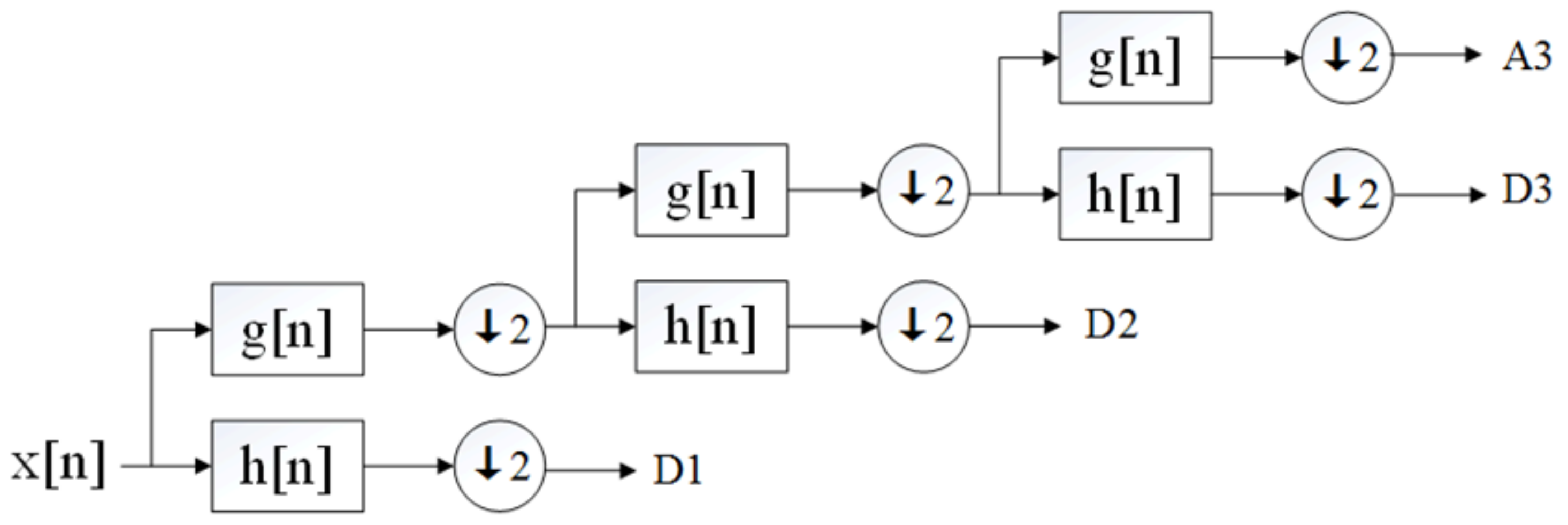
2. Discrete Wavelet Transform

Wavelet transform is often used to analyze instantaneous and time-varying signals. Although a classical Fourier transform can reflect the overall connotation of signals, its expression is usually not intuitive enough. As an alternative to Fourier transform, wavelet transform can decompose signals at different scales. Different decomposition scales can be selected for different processing targets. Moreover, the time and the frequency domains can be simultaneously located. For non-stationary signal analysis, it has great advantages.
Discrete wavelet transform is realized by passing the signal through a series of low-pass and high-pass filters [21,22]. Wavelet transform decomposes the signal into detailed components and approximates components of different scales. Figure 1 is a schematic diagram of discrete wavelet transform, where x [ n ] is the discrete input signal with length n; g [ n ] is a low-pass filter, which can filter out the high-frequency part of the input signal and output the low-frequency part. h [ n ] is a high-pass filter. Contrary to the low-pass filter, it filters out the low-frequency part and outputs the high-frequency part. ↓ is a down-sampling filter.
At present, many wavelet bases have been developed, such as Haar, Daubechies (Db), Symlet and so on, for the analysis and synthesis of signals. Correct selection of a wavelet basis function plays an important role in de-noising performance [23]. Table 1 shows the comparison of the signal-to-noise ratio (SNR) and the mean square error (MSE) of the de-noised ECG signals which are de-noised by several typical wavelet basis. It can be seen from the table that SNR of db5 is relatively high and MSE is relatively low. Therefore, we select db5 as a wavelet basis in the process of de-noising ECG signal in the paper.

3. The Proposed Approach

The framework of the proposed approach is shown in Figure 2. The wavelet coefficients that required threshold de-noising are determined by wavelet energy, and then further de-noising through sub-band smoothing filter to obtain the final de-noised smoothed ECG signal. A detailed explanation on every step is provided below.

3.1. Pre-Processing

It is firstly preprocessed by zero averaging before the wavelet decomposition of the signal. The purpose is to remove the DC component in the signal and make the amplitude of the zero-frequency signal very small. In the subsequent power spectrum analysis, the influence of DC energy on the spectrum analysis of low and intermediate frequency signals can be reduced. The zero averaging formula is given as follows:
X = X m e a n ( X )
where X is the original input signal, m e a n ( X ) represents the mean of X.
The algorithm defaults a tolerance value of 3. Tolerance value is an empericial value, which is adopted to determine the maximum boundary value of the engery change points. For example, if the tolerence value is 3, the position value of the energy change point cannot exceed 3. That is, if the minimum point of energy change occurs at the fourth position, the coefficients of the forward three decompositions are only considered.

3.2. De-Noising Based on Wavelet Engery

3.2.1. Wavelet Decomposition of ECG

Multi-scale and multi-level wavelet decomposition is performed on the signal after the averaging process. As is known to all, the determination of the number of layers of wavelet decomposition affects the subsequent de-noising effect to a certain extent.
If the number of decomposition layers is too small, the de-noising effect will be unsatisfactory. Generally, in order to eliminate high-frequency noise and extract low-frequency components, the number of decomposition layers will be increased to some extent [21], if the number of layers are too high, the error will be considered as large; moreover, it mainly focuses on the reflection of the characteristics of the wavelet basis rather than the signal being analyzed itself, which results in false frequencies and much information loss. For purpose of obtaining more wavelet coefficients, the number of decomposition layers can be appropriately increased, but when the number of decomposition layers is too much, it is easy to cause false frequency.

3.2.2. Calculating the Energy of Each Decomposition Layer

Firstly, the detail coefficients of each layer are calculated according to the detcoef function of Matlab, and then the energy contained in the detail coefficients of each layer is calculated. The calculation formula is as follows:
E j = l o g e i = 0 N c o f i 2
where E j represents the detail coefficient energy of the jth layer, N represents the number of detail coefficient of the jth layer, and c o f i represents the ith detail coefficient of the jth layer.

3.2.3. Selecting the Required De-Noising Points

According to the coefficient energy of each layer calculated above, the wavelet energy curve can be obtained, and then the position of the maximum and minimum points of the energy curve can be calculated, that is the decomposition level where they are.
According to the positions of the maximum and minimum points of the calculated wavelet energy curve, the variation points of the number of detail layers that need to be de-noised can be judged. The previous level of the variation points is considered to be de-noised, while the level of the variation point and the subsequent level are not considered to de-noise.
In practical processing, we only locate the initial several detail coefficients that required processing, without considering the low-frequency components behind.Therefore the first position of the energy change point is particularly important. Selecting the location points required de-noising is divided into the following cases:
  • When the minimum and maximum values of the energy curve exist simultaneously:
    • When the locationof the first maximum point is less than the location of the first minimum point and the location of the first maximum point is less than the median value of the location of the first maximum point and the location of the first minimum point (If the median is not an integer, round to zero).
      When the position of the first maximum point is greater than the tolerance value, the location point is calculated as:
      c h g _ l o c s = m a x _ l o c s ( 1 ) 2
      When the position of the first maximum point is less than the tolerance value, the location point is calculated as
      c h g _ l o c s = m a x _ l o c s ( 1 )
      where c h g _ l o c s is the location point to be determined and m a x _ l o c s ( 1 ) is the location of the first maximum point.
    • When the location of the first maximum point is greater than the location of the first minimum point, and the position of the first minimum point is less than the median value of the position of the first maximum point and the position of the first minimum point.
      When the position of the first minimum point is greater than the tolerance value, the location point is calculated as:
      c h g _ l o c s = m i n _ l o c s ( 1 ) 2
      When the position of the first minimum point is less than the tolerance value, the location point is calculated as:
      c h g _ l o c s = m i n _ l o c s ( 1 )
      where m i n _ l o c s ( 1 ) is the location of the first minimum point.
  • When the minimum point of the energy curve exists and the maximum point does not exist.
    • When the position of the first minimum point is greater than the tolerance value, the location point is calculated as:
      c h g _ l o c s = m i n _ l o c s ( 1 ) 2
    • When the position of the first minimum point is less than the tolerance value, the location point is calculated as:
      c h g _ l o c s = m i n _ l o c s ( 1 )
  • When the maximum point of the energy curve exists and the minimum point does not exist.
    • when the position of the first maximum point is greater than the tolerance value, the location point is calculated as:
      c h g _ l o c s = m a x _ l o c s ( 1 ) 2
    • When the position of the first maximum point is less than the tolerance value, the location point is calculated as:
      c h g _ l o c s = m a x _ l o c s ( 1 )
  • When the minimum and maximum of the energy curve do not exist, we consider that the default noise only appears in the first and second high frequency detail components, and the locating point is set as follows:
    c h g _ l o c s = 3

3.2.4. Threshold De-Noising

When the location point required de-noising is selected, the detail coefficients of each layer before the location point are de-noised using threshold. Hard threshold and soft threshold are adopted in this paper. In hard threshold processing, when the absolute value of the wavelet coefficients is less than the given threshold, it will be zero; when the wavelet coefficients are larger than the given threshold, it will remain unchanged. That is as follows:
ω = ω ω λ 0 ω < λ
where ω is a certain wavelet coefficient and λ is a given threshold.
In soft threshold processing, when the absolute value of the wavelet coefficient is less than the given threshold value, set it as zero; If it is larger than the given threshold value, let the wavelet coefficient subtract the threshold value.That is as follows:
ω = s g n ω ω λ ω λ 0 ω < λ
Hard threshold is superior to soft threshold in mean square error, however, the signal will produce additional oscillation and jump point, which does not have the smoothness of the original signal. The wavelet coefficients obtained by soft threshold have good continuity and the tested signal will not produce additional oscillation. However, due to the compression of the signal, there will be a certain deviation, which directly affects the approximation level between the reconstructed signal and the real signal. We adopt a fixed threshold to signal de-noising, and the formula is as follows:
λ = σ 2 l o g N
where λ is the threshold, N is the number of samples, and σ is the noise standard deviation. The noise standard deviation is calculated separately according to each layer, and the values are different in the threshold processing of different layers.

3.3. Signal Reconstruction

According to the detailed coefficients of the location point layer and the following layer of the wavelet decomposition, and the detail coefficients from the first layer to the front layer of the locating point after threshold de-noising, and the approximate coefficients, the signal is reconstructed by the wavelet transform, which is the inverse discrete wavelet transform.

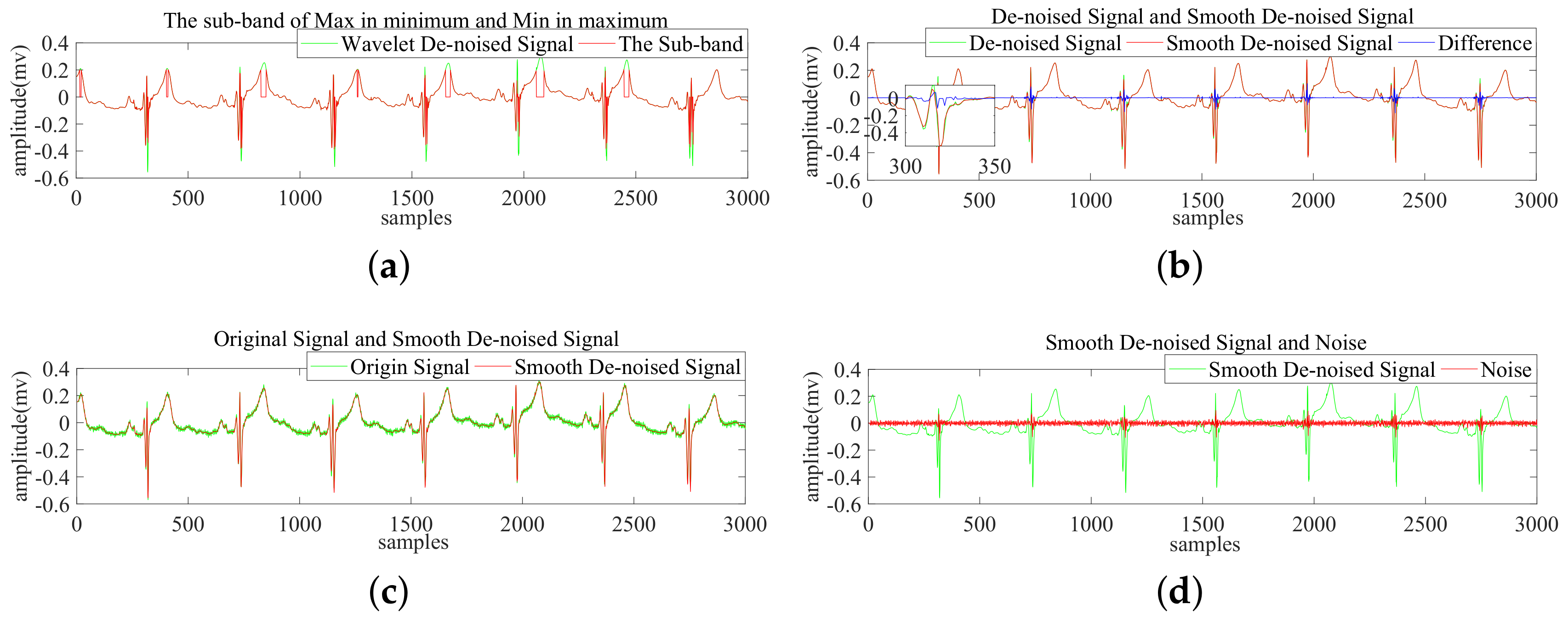
3.4. signal Smoothing Processing

After threshold de-noising and wavelet reconstruction, some noises still exist in the reconstructed ECG signal. These noises are clearly visible in the low time varying components of the ECG signal i.e., the region between QRS complexes. Therefore, signal smoothing processing is applied for further enhancement of ECG signal quality. In this paper, we determine the subband information required smoothing by the subbands divided by the maximum of the minimum values and the minimum of the maximum values of reconstructed signal. We define lmax as the maximum of the minimum values of reconstructed signal, and upmin as the minimum of the maximum values of reconstructed signal. The reconstructed signal is smoothed point by point from the second point, the processing can be divided into the following situations:
  • when the i t h point of the signal, i.e., s i g ( i ) , is between lmax and upmin, consider its previous point s i g ( i 1 ) and the next point s i g ( i + 1 ) , and the filtering is as follows:
    • when both s i g ( i 1 ) and s i g ( i + 1 ) are between lmax and upmin, the smoothing filter formula is:
      s i g i = s i g i 1 + s i g i + s i g i + 1 3
    • when s i g ( i 1 ) is between lmax and upmin, and s i g ( i + 1 ) is not between lmax and upmin, the smoothing filter formula is:
      s i g i = s i g i 1 + s i g i 2
    • when s i g ( i + 1 ) is between lmax and upmin, and s i g ( i 1 ) is not between lmax and upmin, the smoothing filter formula is:
      s i g i = s i g i + s i g i + 1 2
    • when both s i g ( i 1 ) and s i g ( i + 1 ) are not between lmax and upmin, the smoothing filter formula is:
      s i g i = s i g i
  • When the ith point of the signal, i.e., s i g ( i ) , is not between lmax and upmin, the smoothing filter formula is:
    s i g i = s i g i

4. Results and Discussion

4.1. Experimental Environment

To verify the performance of the proposed algorithm, we conduct a number of experiments in our personal computer. The presented approach is implemented in Matlab2012b. We use MIT-BIH arrhythmia database [24] as a reference for real signals. Each sample length is 650,000. The sampling rate is 360 Hz and the resolution is 11 bps. For simulated electrocardiograms, we used the introduced dynamic model to generate synthetic ECG signals [25,26].
In the qualitative evaluation, we select the signal numbered 114 for direct de-noising observation because the record contains more noise. In addition, since there is an ectopic complexes in 119 record, we add noise to record 119 and compared the effect of de-noising with several traditional methods. Finally, In order to observe the de-noising effect of this method under different types of noise, we add power line interference, Gaussian noise and EMG noise to records 106, 113 and 115, respectively.
In the quantitative evaluation, we consider ECG signals such as 100, 103, 105, 113, 115, 117, 119, 122, 200, 215, 230, which contain time-varying QRS morphology, normal and abnormal ECG beats. In each set of experiments, these signals are tested 100 times and averaged. In addition, the record 115 is quantitatively evaluated by adding different types of noise.
We simulated power line interference, EMG noise and synthetic interference. In order to evaluate the performance of the proposed method for power line interference denoising, the additional functions of these interference are as follows:
N t = A × sin 2 π f t
where A = 0.15 m v and f = 50 HZ . The signal was added to the original electrocardiogram signal to simulate power line interference. Random noise is added to ecg signals [27] to simulate EMG interference ( μ = 0 , σ = 0.15 ). In the case of synthetic interference, white gaussian noise (WGN) is used to simulate these noises.

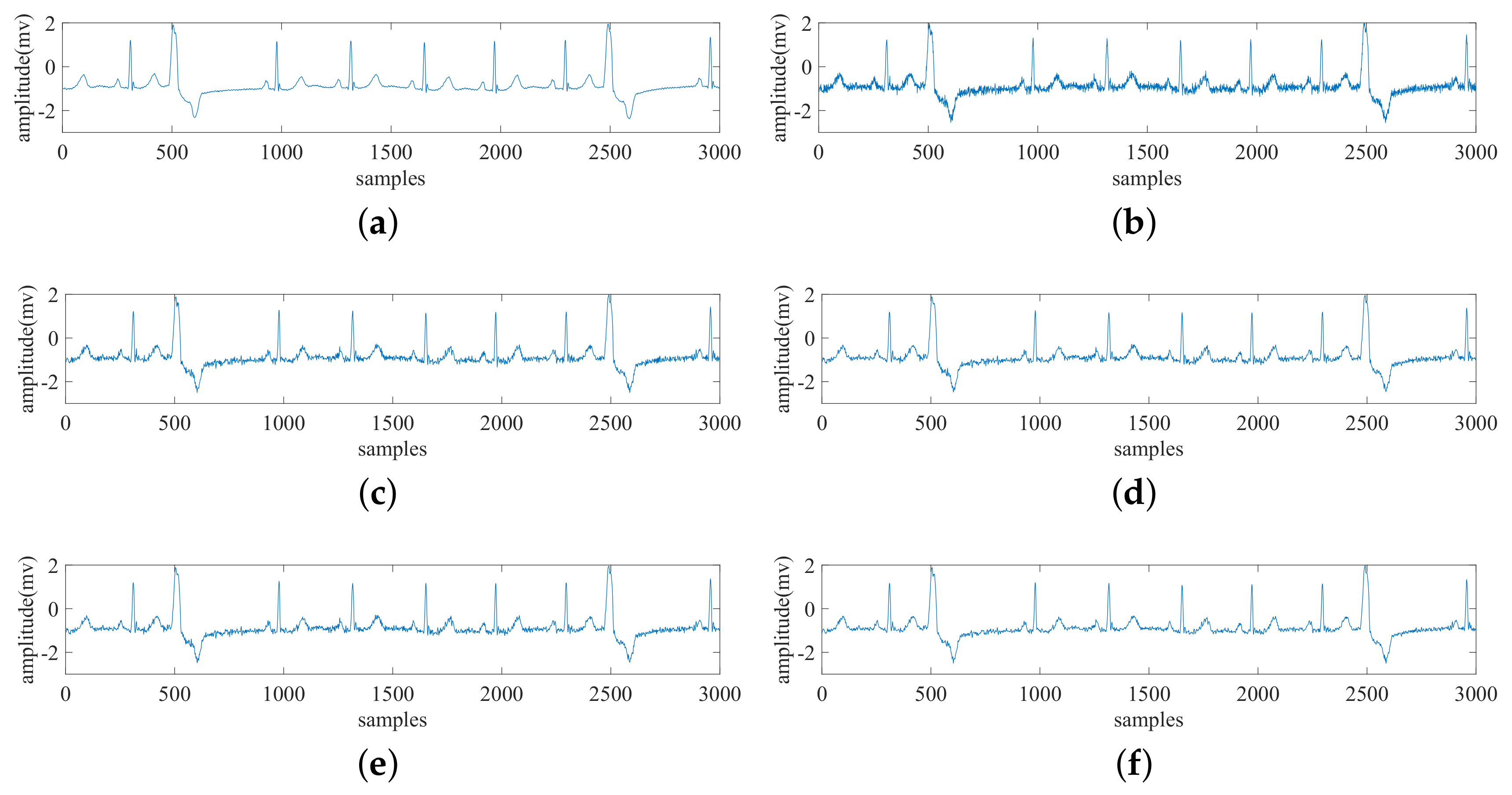
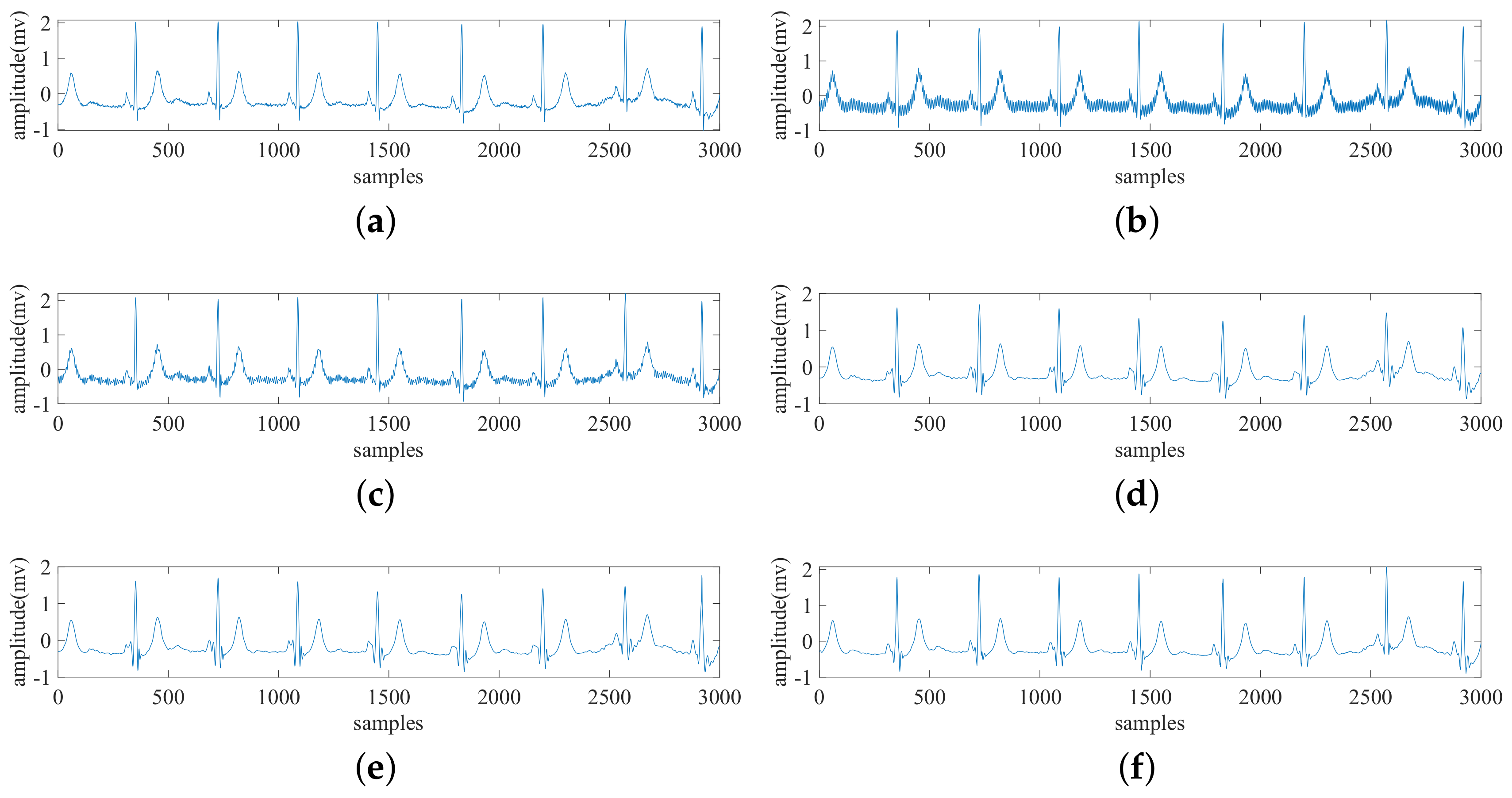
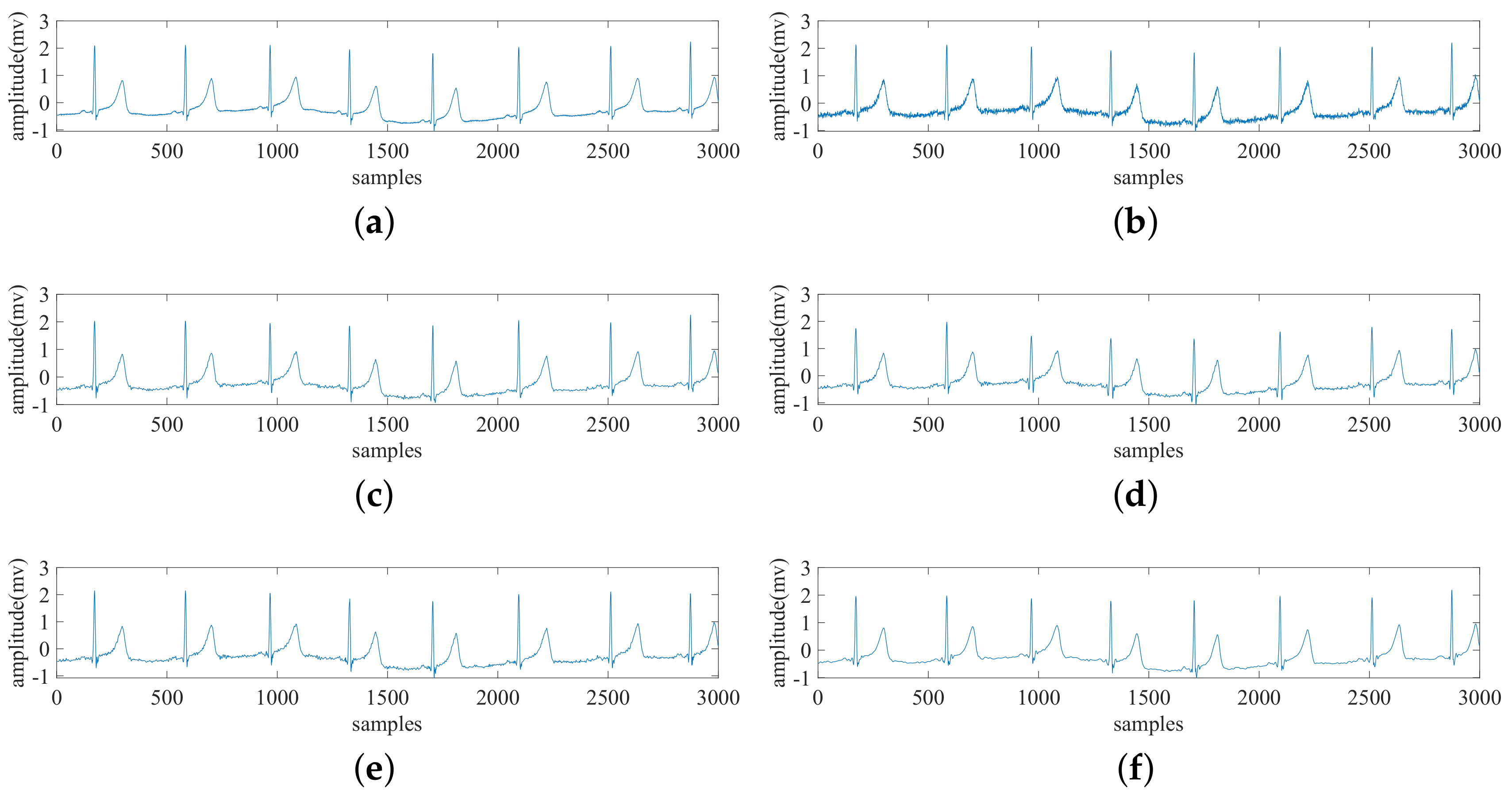
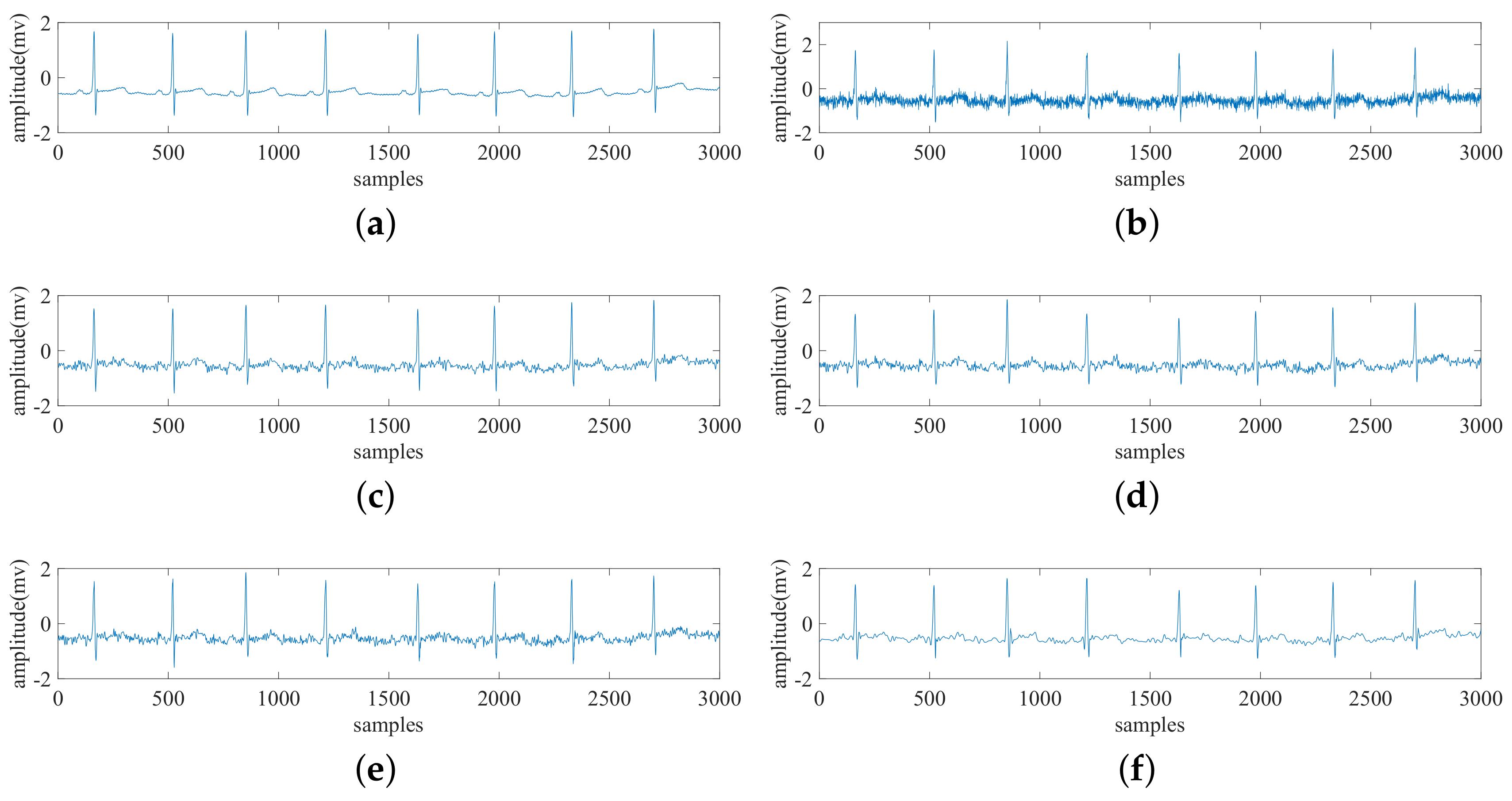
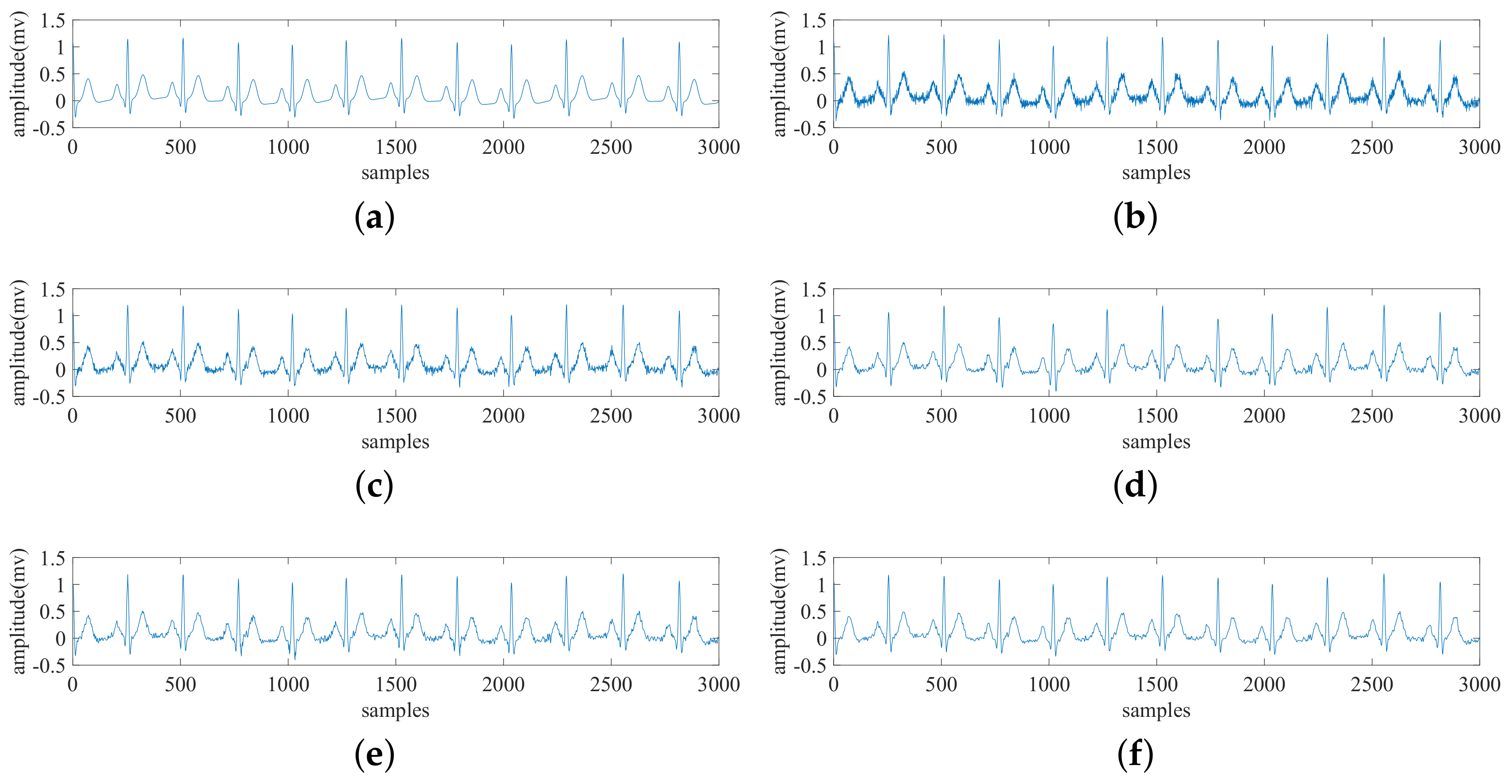
4.2. Qualitative Evaluation

The performance of the proposed de-noising algorithm is qualitatively analyzed by visual evaluation. Figure 3 shows the results of de-noising the No. 114 record in the MIT-BIH database. As can be seen from the figure, the signal that is de-noised by wavelet obviously reduces a lot of noise, while the signal smoothed further removes more noise.
In Figure 4, we select 119 records from the MIT-BIH arrhythmia database, which contained some ectopic complexs (there exists a complex in the opposite direction of QRS complex before the appearance of QRS complex, called as ectopic complex). We add 20 dB of white Gaussian noise to it to destroy the record. It can be observed from the denoised signals that these ectopic complexes are still preserved in the reconstructed signals, which will not affect the analysis of ECG signals. Compared with the traditional wavelet de-noising, EMD and EMD soft threshold, the ECG signal de-noised by the proposed method is closer to the original ECG signal and smoother.
Figure 5, Figure 6 and Figure 7 demonstrate the de-noising effect of the proposed method for various noises. Figure 5 shows the de-noising results of signal after adding 50 HZ power line interference to No. 106 record of the MIT-BIH database. Figure 6 displays the results of adding 20 dB WGN to No. 113 record of the MIT-BIH database. Figure 7 shows the de-noising results after adding EMG interference to No. 115 record of the MIT-BIH database. As can be seen from these figures, the de-noising effect is obvious and the distortion is smaller than that of the original signal. The results show that the proposed method can effectively de-noise all kinds of noises, and the de-noised signal retains the characteristics of the original signal. Moreover the signal is very similar to the original signal.
The evaluation also extends to the synthetic ECG signal. We add 15 dB Gauss white noise to the synthetic signal and denoise it. As shown in Figure 8, it can be seen that the algorithm also has excellent denoising effect on the synthetic ECG signal.

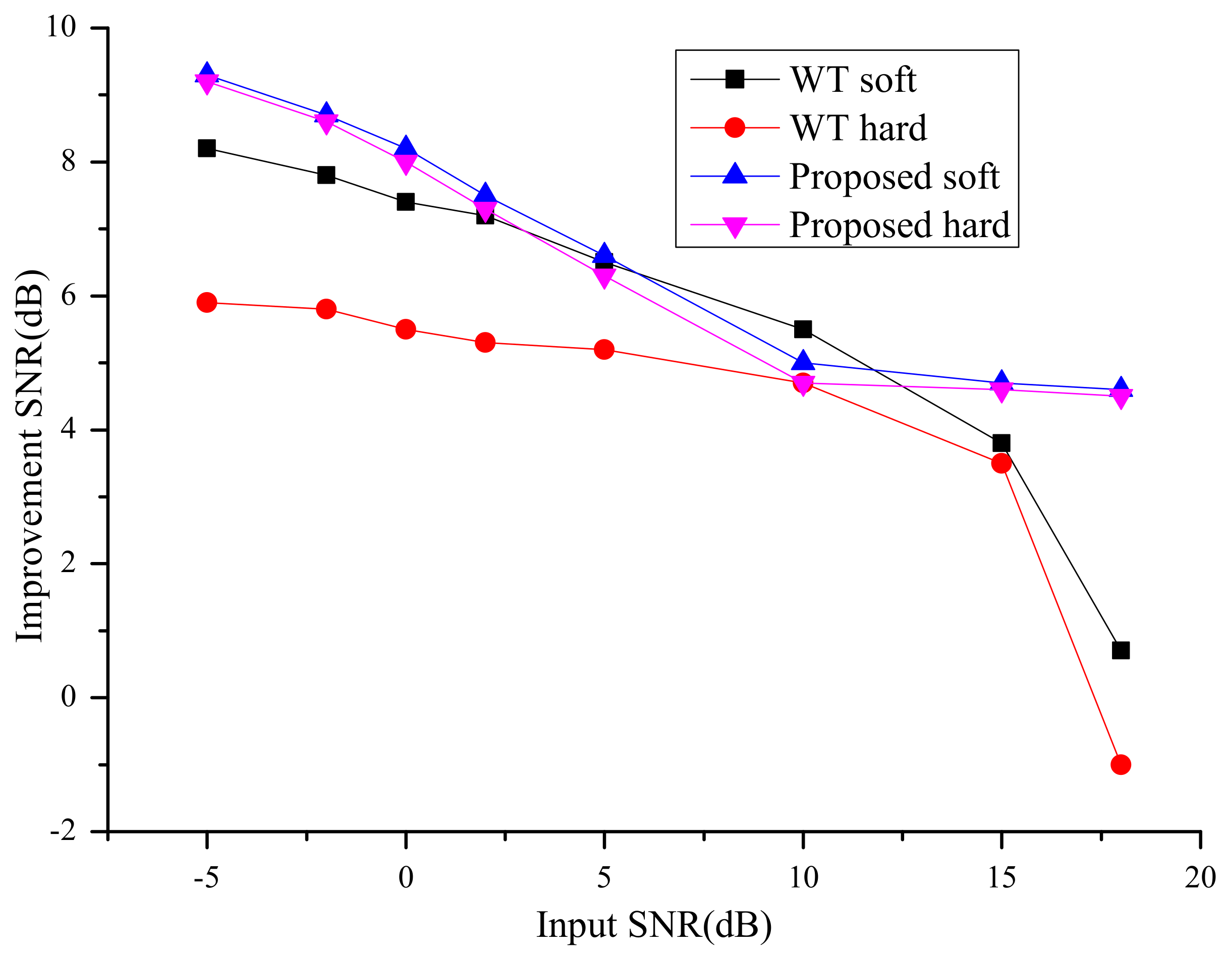
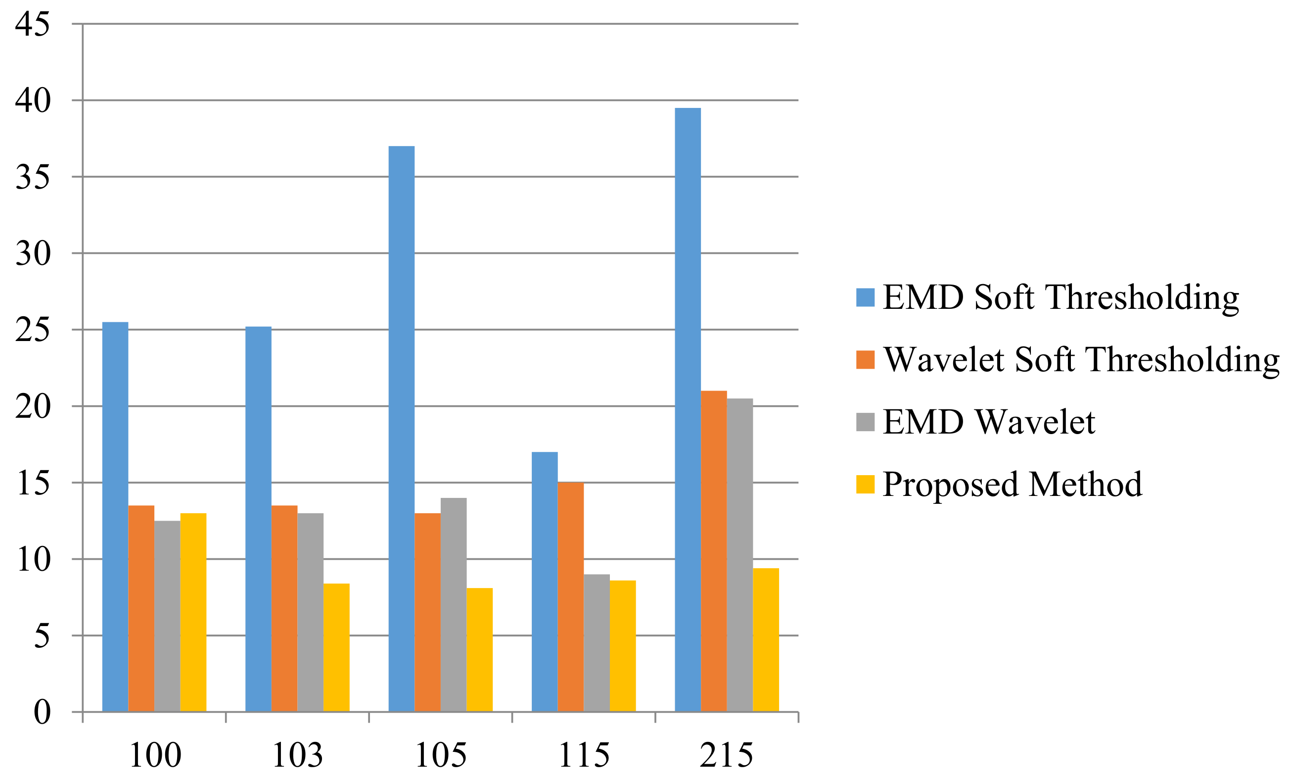
4.3. Quantitative Comparison

In this paper, the performance of de-noising signal is analyzed by SNR, MSE and PRD, and the quality of reconstructed signal is studied. The SNR can be divided into output SNR and improved SNR.
The output SNR formula is defined as follows:
S N R o u t = 10 l g i = 1 L x 2 i i = 1 L s i x i 2
The formula of improved SNR is defined as follows:
S N R i m p = 10 l g i = 1 L y i x i 2 i = 1 L s i x i 2
The MSE is used to measure the deviation between the original signal and the de-noised signal. The formula is given as follows:
M S E = 1 L i = 1 L x i s i 2
The percent root mean square difference is defined as follows:
P R D = i = 1 L x i s i 2 i = 1 L x 2 i × 100
where x i is the original signals, y i is the signal after adding noise, s i is the final de-noised and smoothed signal, and L is the signal length.
The experimental comparison shows that the de-noising effect is better when the wavelet basis of DB family is used for wavelet transform. In order to compare with the traditional wavelet-based ECG de-noising scheme, we tested the traditional wavelet-based ECG de-noising scheme (WT), multi-adaptive bionic wavelet transform (MABWT) and our proposed method in MIT-BIH arrhythmia database [28]. Table 2 (Soft Threshold) and Table 3 (Hard Threshold) respectively show the improved SNR results of ECG signals de-noising with WGN (5 dB) added. It can be seen that compared with the traditional wavelet-based de-noising scheme and multi-adaptive bionic wavelet transform, the method proposed in this paper has a higher SNR improvement whether it uses soft threshold or hard threshold.
Table 4, Table 5 and Table 6 shows the results of quantitative comparison with several other methods after adding different noise to the 115th record for denoising, namely, the parallel-type fractional zero-phase filtering (FZP), zero-phase Butterworth filter (BZP) [29], the Riemann Liouville (RL) integrator [30] and the proposed method. We select record 115 because the record is relatively clean and suitable for observing the de-noising effect of the algorithm on different types of noise. Table 4 gives a comparison of power line interference (50 Hz), with an amplitude of 0.15 mv. In Table 5, EMG interference is compared and these noises are simulated using random noise. Table 6 gives the comparison results in the case of synthetic interference. These noises are simulated using WGN with an input signal-to-noise ratio of 15 dB. Table 4, Table 5 and Table 6 shows that the proposed algorithm provides better de-noising results and has smaller deviation compared with the original ECG signal. The ability of the algorithm in tracking signal and removing noise is proved.
Figure 9 illustrates the comparison between the proposed de-noising method and the traditional wavelet de-noising method (soft threshold and hard threshold) for a wide range of input SNR [28]. It can be observed that for low SNR, the proposed method has a high improvement SNR. With the increase of the input SNR, the improved SNR is still high and stable. Unlike traditional wavelet denoising, the improved SNR is very low or even negative for high input SNR.
Table 7 and Figure 10 show the comparison of the proposed method with EMD soft threshold [4], wavelet soft threshold [12] and EMD-wavelet [13]. Table 7 shows the results of the MSE for all the comparison methods using different ECG signals under consideration at a particular input SNR level of 20 dB. It is vivid from this table that the proposed method yields the smallest MSE and verify its capability to yield enhanced ECG signal with better quality. A bar diagram presenting the percentage PRD(%) results obtained by using different de-noising methods are plotted in Figure 10. We add Gauss white noise with input signal-to-noise ratio of 20 dB to ECG signal. The histogram clearly shows that the proposed method performs best for any ECG signal because it yields the lowest PRD(%).

5. Conclusions

Wavelet transform is a signal analysis tool. The tight support and orthogonality of wavelet function cause it to have good performance in signal de-noising. A new de-noising method of ECG signals based on wavelet energy and sub-band smoothing is proposed in this paper. The wavelet coefficients that required threshold de-noising are determined by wavelet energy, and then the sub-band smoothing filter is used for further de-noising. The experimental results show that the proposed method can significantly improve the quality of ECG signal, and the de-noising results have higher SNR, lower MSE and lower PRD. In the future, we will attempt to adopt the image/video processing methods [31,32,33,34,35,36,37,38] to process ECG signal. With the wide application of deep learning in image processing, We will adopt network optimization methods [39,40,41,42,43,44,45,46,47,48] to improve the real-time and high efficiency performance of ECG signal processing.

Author Contributions

Conceptualization: D.Z. and S.W.; investigation: J.W.; methodology: D.Z. and S.W.; software: D.Z. and S.W.; supervision: F.L.; validation: A.K.S. and V.S.S.; Writing—Original draft: D.Z. and S.W.; Writing—Review and editing: J.W., A.K.S. and X.D.

Funding

This research was funded by the National Natural Science Foundation of China (61772454, 61811530332, 61811540410, 61772087, 61232016,61972057, U1836208), the “Double First-class” International Cooperation and Development Scientific Research Project of Changsha University of Science and Technology (No. 2018IC25) and the Young Teacher Growth Plan Project of Changsha University of Science and Technology(No. 2019QJCZ076), Hunan Provincial Natural Science Foundation of China(No.2019JJ50655,2019JJ50649), Scientific Research Foundation of Hunan Provincial Education Department of China (No.18B160,18C0238),Open Fund of Hunan Key Laboratory of Smart Roadway and Cooperative Vehicle Infrastructure Systems (Changsha University of Science and Technology) (No. kfj180402).

Conflicts of Interest

The authors declare no conflict of interest.

References

  1. Scheidt, S.; Netter, F.H. Basic Electrocardiography; CIBA-GEIGY Pharmaceuticals: West Caldwell, NJ, USA, 1986. [Google Scholar]
  2. Jenkal, W.; Latif, R.; Toumanari, A.; Dliou, A.; El B’charri, O.; Maoulainine, F.M. An efficient algorithm of ECG signal denoising using the adaptive dual threshold filter and the discrete wavelet transform. Biocybern. Biomed. Eng. 2016, 36, 499–508. [Google Scholar] [CrossRef]
  3. Huang, N.E.; Shen, Z.; Long, S.R.; Wu, M.C.; Shih, H.H.; Zheng, Q.; Yen, N.C.; Tung, C.C.; Liu, H.H. The empirical mode decomposition and the Hilbert spectrum for nonlinear and non-stationary time series analysis. Proc. R. Soc. Lond. Ser. A Math. Phys. Eng. Sci. 1998, 454, 903–995. [Google Scholar] [CrossRef]
  4. Tang, G.T.G.; Qin, A.Q.A. ECG De-noising Based on Empirical Mode Decomposition. In Proceedings of the 2008 The 9th International Conference for Young Computer Scientists, Hunan, China, 18–21 November 2008. [Google Scholar]
  5. Sayadi, O.; Shamsollahi, M.B. ECG denoising and compression using a modified extended Kalman filter structure. IEEE Trans. Biomed. Eng. 2008, 55, 2240–2248. [Google Scholar] [CrossRef] [PubMed]
  6. Cuomo, S.; De Pietro, G.; Farina, R.; Galletti, A.; Sannino, G. A revised scheme for real time ECG Signal denoising based on recursive filtering. Biomed. Signal Process. Control 2016, 27, 134–144. [Google Scholar] [CrossRef]
  7. Poornachandra, S.; Kumaravel, N. A novel method for the elimination of power line frequency in ECG signal using hyper shrinkage function. Digit. Signal Process. 2008, 18, 116–126. [Google Scholar] [CrossRef]
  8. Poornachandra, S.; Kumaravel, N. Hyper-trim shrinkage for denoising of ECG signal. Digit. Signal Process. 2005, 15, 317–327. [Google Scholar] [CrossRef]
  9. Singh, O.; Sunkaria, R.K. ECG signal denoising based on empirical mode decomposition and moving average filter. In Proceedings of the 2013 IEEE International Conference on Signal Processing, Computing and Control (ISPCC), Solan, India, 26–28 September 2013; pp. 1–6. [Google Scholar]
  10. Donoho, D.L.; Johnstone, J.M. Ideal spatial adaptation by wavelet shrinkage. Biometrika 1994, 81, 425–455. [Google Scholar] [CrossRef]
  11. Donoho, D.L. De-noising by soft-thresholding. IEEE Trans. Inf. Theory 1995, 41, 613–627. [Google Scholar] [CrossRef]
  12. Alfaouri, M.; Daqrouq, K. ECG Signal Denoising By Wavelet Transform Thresholding. Am. J. Appl. Sci. 2008, 5, 276–281. [Google Scholar] [CrossRef]
  13. Kabir, M.A.; Shahnaz, C. Denoising of ECG signals based on noise reduction algorithms in EMD and wavelet domains. Biomed. Signal Process. Control 2012, 7, 481–489. [Google Scholar] [CrossRef]
  14. Patil, H.T.; Holambe, R.S. New approach of threshold estimation for denoising ECG signal using wavelet transform. In Proceedings of the 2013 Annual IEEE India Conference (INDICON), Mumbai, India, 13–15 December 2013; pp. 1–4. [Google Scholar]
  15. Bouny, L.E.; Khalil, M.; Adib, A. ECG signal denoising based on ensemble emd thresholding and higher order statistics. In Proceedings of the 2017 International Conference on Advanced Technologies for Signal and Image Processing (ATSIP), Fez, Morocco, 22–24 May 2017. [Google Scholar]
  16. Rakshit, M.; Das, S. An efficient ECG denoising methodology using empirical mode decomposition and adaptive switching mean filter. Biomed. Signal Process. Control 2018, 40, 140–148. [Google Scholar] [CrossRef]
  17. Zhou, P.; Zhang, X. A novel technique for muscle onset detection using surfaceemg signals without removal of ECG artifacts. Physiol. Meas. 2014, 35, 45–54. [Google Scholar] [CrossRef] [PubMed]
  18. Barrios-Muriel, J.; Romero, F.; Alonso, F.J.; Gianikellis, K. A simple SSA-based denoising technique to remove ECG interferencein EMG signals. Biomed. Signal Process. Control 2016, 30, 117–126. [Google Scholar] [CrossRef]
  19. Yang, B.; Yu, C.; Dong, Y. Capacitively coupled electrocardiogram measuring system and noise reduction by singular spectrum analysis. IEEE Sens. J. 2016, 16, 3802–3810. [Google Scholar] [CrossRef]
  20. Mortezaee, M.; Mortezaie, Z.; Abolghasemi, V. An Improved SSA-Based Technique for EMG Removal from ECG. IRBM 2019, 40, 62–68. [Google Scholar] [CrossRef]
  21. Mallat, S. A Wavelet Tour of Signal Processing; Academic Press: San Diego, CA, USA, 1998. [Google Scholar]
  22. Von Borries, R.; Pierluissi, J.H.; Nazeran, H. Redundant discrete wavelet transform for ECG signal processing. Biomed. Soft Comput. Hum. Sci. 2009, 14, 69–80. [Google Scholar]
  23. Gokhale, P.S. ECG Signal De-noising using Discrete Wavelet Transform for removal of 50 Hz PLI noise. Int. J. Emerg. Technol. Adv. Eng. 2012, 2, 81–85. [Google Scholar]
  24. The MIT-BIH Arrhythmia Database. Available online: https://www.physionet.org/content/mitdb/1.0.0/ (accessed on 24 February 2005).
  25. McSharry, P.E.; Clifford, G.D.; Tarassenko, L.; Smith, L.A. A dynamical model for generating synthetic electrocardiogram signals. IEEE Trans. Biomed. Eng. 2003, 50, 289–294. [Google Scholar] [CrossRef]
  26. McSharry, P.E.; Clifford, G.D. ECGSYN-A Realistic ECG Waveform Generator. 2003. Available online: http://www.physionet.org/physiotools/ecgsyn (accessed on 3 December 2003).
  27. Khaing, A.S.; Naing, Z.M. Quantitative investigation of digital filters in electrocardiogram with simulated noises. Int. J. Inf. Electron. Eng. 2011, 1, 210–216. [Google Scholar]
  28. Sayadi, O.; Shamsollahi, M.B. Multiadaptive bionic wavelet transform: Application to ECG denoising and baseline wandering reduction. EURASIP J. Adv. Signal Process. 2007, 2007, 041274. [Google Scholar] [CrossRef]
  29. Wang, J.; Ye, Y.; Pan, X.; Gao, X. Parallel-type fractional zero-phase filtering for ECG signal denoising. Biomed. Signal Process. Control 2015, 18, 36–41. [Google Scholar] [CrossRef]
  30. Wang, J.; Ye, Y.; Pan, X.; Gao, X.; Zhuang, C. Fractional zero-phase filtering based on the Riemann-Liouville integral. Signal Process. 2014, 98, 150–157. [Google Scholar] [CrossRef]
  31. Tang, D.; Zhou, S.; Yang, W. Random-filtering based sparse representation parallel face recognition. Multimed. Tools Appl. 2019, 78, 1419–1439. [Google Scholar] [CrossRef]
  32. Tirkolaee, E.; Hosseinabadi, A.; Soltani, M.; Sangaiah, A.; Wang, J. A Hybrid Genetic Algorithm for Multi-trip Green Capacitated Arc Routing Problem in the Scope of Urban Services. Sustainability 2018, 10, 1366. [Google Scholar] [CrossRef]
  33. Chen, Y.; Wang, J.; Chen, X.; Zhu, M.; Yang, K.; Wang, Z.; Xia, R. Single-Image Super-Resolution Algorithm Based on Structural Self-Similarity and Deformation Block Features. IEEE Access 2019, 7, 58791–58801. [Google Scholar] [CrossRef]
  34. Zhang, J.; Jin, X.; Sun, J.; Wang, J.; Sangaiah, A.K. Spatial and semantic convolutional features for robust visual object tracking. Multimed. Tools Appl. 2018. [Google Scholar] [CrossRef]
  35. Zhang, J.; Jin, X.; Sun, J.; Wang, J.; Li, K. Dual model learning combined with multiple feature selection for accurate visual tracking. IEEE Access 2019, 7, 43956–43969. [Google Scholar] [CrossRef]
  36. Song, Y.; Yang, G.; Xie, H.; Zhang, D.; Sun, X. Residual domain dictionary learning for compressed sensing video recovery. Multimed. Tools Appl. 2017, 76, 10083–10096. [Google Scholar] [CrossRef]
  37. Xiang, L.; Shen, X.; Qin, J.; Hao, W. Discrete Multi-Graph Hashing for Large-scale Visual Search. Neural Process. Lett. 2019, 49, 1055–1069. [Google Scholar] [CrossRef]
  38. Sun, H.; Gao, C.; Zhang, Z.; Liao, X.; Wang, X.; Yang, J. High-resolution anisotropic prestack Kirchhoff dynamic focused beam migration. IEEE Sens. J. 2019. [Google Scholar] [CrossRef]
  39. Nguyen, T.T.; Pan, J.S.; Dao, T.K. An Improved Flower Pollination Algorithm for Optimizing Layouts of Nodes in Wireless Sensor Network. IEEE Access 2019, 7. [Google Scholar] [CrossRef]
  40. Wang, J.; Gao, Y.; Liu, W.; Sangaiah, A.K.; Kim, H.J. An Intelligent Data Gathering Schema with Data Fusion Supported for Mobile Sink in WSNs. Int. J. Distrib. Sens. Netw. 2018, 15. [Google Scholar] [CrossRef]
  41. Wang, J.; Cao, J.; Sherratt, R.S.; Park, J.H. An improved ant colony optimization-based approach with mobile sink for wireless sensor networks. J. Supercomput. 2018, 74, 6633–6645. [Google Scholar] [CrossRef]
  42. Wang, J.; Cao, J.; Ji, S.; Park, J.H. Energy Efficient Cluster-based Dynamic Routes Adjustment Approach for Wireless Sensor Networks with Mobile Sinks. J. Supercomput. 2017, 73, 3277–3290. [Google Scholar] [CrossRef]
  43. Wang, J.; Gao, Y.; Yin, X.; Li, F.; Kim, H.J. An Enhanced PEGASIS Algorithm with Mobile Sink Support for Wireless Sensor Networks. Wirel. Commun. Mob. Comput. 2018, 2018, 9472075. [Google Scholar] [CrossRef]
  44. Wang, J.; Gao, Y.; Liu, W.; Wu, W.; Lim, S.J. An Asynchronous Clustering and Mobile Data Gathering Schema based on Timer Mechanism in Wireless Sensor Networks. Comput. Mater. Contin. 2019, 58, 711–725. [Google Scholar] [CrossRef] [Green Version]
  45. Pan, J.S.; Lee, C.Y.; Sghaier, A.; Zeghid, M.; Xie, J. Novel Systolization of Subquadratic Space Complexity Multipliers Based on Toeplitz Matrix-Vector Product Approach. IEEE Trans. Very Large Scale Integr. Syst. 2019, 27, 1614–1622. [Google Scholar] [CrossRef]
  46. He, Y.; Xiang, S.; Li, K.; Liu, Y. Region-Based Compressive Networked Storage with Lazy Encoding. IEEE Trans. Parallel Distrib. Syst. 2019, 30, 1390–1402. [Google Scholar]
  47. Pan, J.S.; Kong, L.; Sung, T.W.; Tsai, P.W.; Snášel, V. Alpha-Fraction First Strategy for Hierarchical Wireless Sensor Networks. J. Internet Technol. 2018, 19, 1717–1726. [Google Scholar]
  48. He, S.; Xie, K.; Chen, W.; Zhang, D.; Wen, J. Energy-aware Routing for SWIPT in Multi-hop Energy-constrained Wireless Network. IEEE Access 2018, 6, 17996–18008. [Google Scholar] [CrossRef]
Figure 1. Wavelet decomposition.
Applsci 09 04968 g001
Figure 2. The framework of the proposed approach.
Applsci 09 04968 g002
Figure 3. The results of de-noising 114 records in the MIT-BIH database: (a) Green is the signal de-noised by wavelet transform (including burrs), and red is the sub-band segmented by the minimum of maximum and the maximum of minimum. (b) The comparison between the signal after wavelet de-noising and the signal after wavelet de-noising and smoothing. (c) The comparison between the original signal and the signal after wavelet de-noising and smoothing. (d) The signal after de-noising and the resulting noise.
Applsci 09 04968 g003
Figure 4. The de-noising results of adding 20 dB WGN to No. 119 record of the MIT-BIH database: (a) The original signal. (b) The signal after adding 20 dB WGN. (cf) De-noised signals using wavelet soft threshold, EMD, EMD soft threshold, proposed method.
Applsci 09 04968 g004
Figure 5. The de-noising results of signal added 50 HZ power line interference to the 106 record of the MIT-BIH database: (a) The original signal. (b) The signal after adding power line interference. (cf) De-noised signals using wavelet soft threshold, EMD, EMD soft threshold, proposed method.
Applsci 09 04968 g005
Figure 6. The de-noising results of adding 20 dB WGN to No. 113 record of the MIT-BIH database: (a) The original signal. (b) The signal after adding 20 dB WGN. (cf) De-noised signals using wavelet soft threshold, EMD, EMD soft threshold, proposed method.
Applsci 09 04968 g006
Figure 7. The de-noising results after adding EMG noise to No. 115 record of the MIT-BIH database: (a) The original signal. (b) The signal after adding EMG noise. (cf) De-noised signals using wavelet soft threshold, EMD, EMD soft threshold, proposed method.
Applsci 09 04968 g007
Figure 8. The de-noising results after adding 15 dB WGN to the synthetic ECG: (a) The original signal. (b) The signal after adding WGN. (cf) De-noised signals using wavelet soft threshold, EMD, EMD soft threshold, proposed method.
Applsci 09 04968 g008
Figure 9. WT and proposed method output SNR improvement versus different input SNRs for the first 4096 samples of the MIT-BIH record number 100.
Applsci 09 04968 g009
Figure 10. Comparison of the PRD(%) obtained by using different de-noising methods.
Applsci 09 04968 g010
Table 1. Comparison of the de-noising results by several typical wavelet basis.
ECG SignalsSNRMSE
db5sym5haarcoif5db5sym5haarcoif5
10022.8721.3819.5320.820.000150.000210.000330.00024
10123.7023.6319.3021.000.000180.000180.000500.00034
10223.1822.8521.7722.720.000140.000150.000200.00016
10326.8426.7821.0726.700.000190.000190.000730.00019
10425.8425.2422.5925.300.000180.000210.000390.00021
Average24.4823.9720.8523.300.000160.000180.000430.00022
Table 2. S N R i m p comparison of de-noising results using soft threshold for ECG signals with WGN (5 dB).
ECG SignalsWTMABWTProposed Method
1006.57.87.1
1036.17.77.9
1056.08.19.4
1156.67.88.0
2156.17.48.6
1136.27.97.7
1176.07.98.0
1195.87.67.8
1225.66.98.5
2005.46.97.7
2305.97.97.0
average6.017.627.97
Table 3. S N R i m p comparison of de-noising results using hard threshold for ECG signals with WGN (5 dB).
ECG SignalsWTMABWTProposed Method
1005.16.46.9
1035.05.87.4
1055.15.89.1
1155.16.37.2
2154.95.58.2
1135.05.97.1
1174.85.87.2
1194.75.67.5
1224.45.28.2
2004.25.37.5
2305.05.66.3
average4.845.747.51
Table 4. The correction results comparison of the power line interferences in the signal 115 of the MIT-BIH database.
RLBZPFZPProposed Method
S N R o u t 6.5410.0614.2516.12
M S E 0.07540.03350.01280.0017
Table 5. The correction results comparison of the EMG interferences in the signal 115 of the MIT-BIH database.
RLBZPFZPProposed Method
S N R o u t 6.839.7913.6810.76
M S E 0.07050.03560.01460.0078
Table 6. The correction results comparison of the synthetic interferences (WGN of 15 dB) in the signal 115 of the MIT-BIH database.
RLBZPFZPProposed Method
S N R o u t 6.779.8113.4714.04
M S E 0.07150.03550.01530.0039
Table 7. Comparison of the MSE obtained by using different denoising methods.
ECG SignalsEMD Soft ThresholdingWavelet Soft ThresholdingEMD WaveletProposed Method
1000.0090.00260.00190.00058
1030.010.0030.00240.00068
1050.02280.0030.00320.00053
1150.00940.00350.00300.00055
2150.01050.00290.00280.0005

