The Influence of Freeze-Thaw Cycles on the Mechanical Properties and Parameters of the Duncan-Chang Constitutive Model of Remolded Saline Soil in Nong’an County, Jilin Province, Northeastern China

Abstract

In seasonally frozen areas, physical and mechanical soil properties change dynamically under the effect of the freeze-thaw cycles (FTCs), which is a problem that cannot be ignored in geotechnical engineering. In order to study the effect of the FTC on the strength and the mechanism of deformation and failure of saline soil, this paper took Nong’an saline soil as the research object. In total, 105 groups of remolded samples with different salt contents (S) after FTCs were examined in unconsolidated-undrained tests. On the basis of the experiment results, the influence of FTCs on the mechanical properties of Nong’an saline soil was analyzed. The failure principal stress difference (σ₁ − σ₃)_f and cohesion (c) were both decreased with FTC. This occurred especially rapidly after the first cycle and became stable between 30 and 60 cycles. The internal friction angle φ increased at first and then decreased. According to experimental data, a modified Duncan-Chang model was established. Compared with the experiment results, this model was reasonable to simulate the stress-strain relationship of Nong’an saline soil. Furthermore, the empirical formulas of Duncan-Chang model parameters were obtained by regression analysis. This provides a theoretical basis for saline–soil foundation and subgrade engineering in seasonal frozen areas.

1. Introduction

In seasonal frozen–soil regions, the freeze-thaw cycle (FTC) is an important factor affecting soil’s physical and mechanical properties [1]. As the temperature decreases, water in soil turns into ice, volume expansion increases pores, and the freezing process leads to aggregate separation and the breaking of soil particles. Changes in soil structure during the freezing process do not completely recover as the temperatures rises [2]. Under the effect of repeated FTCs, the soil structure is repeatedly adjusted, so its physical and mechanical properties are changed, such as porosity [3,4], severity [5], hydrologic properties [6], permeability [7,8], and strength and deformation [9]. Thus, soil mechanical properties are key considerations in construction projects in cold areas.

Because soil- structure changes caused by FTCs have a significant influence on soil properties, there are many previous studies on shear-strength changes of soils after FTCs [5,9,10,11]. In one, the expansive soil remained stable after the first cycle, but soil volume increased, and c and φ decreased as the number of FTCs increased [5]. In another, the elastic modulus, failure strength, and c and φ of silt sand varied with the increase of FTCs [9]. One study showed that the shear strength of saline-soil samples decreased with the increase of S, and long-term FTC could break down soil particles and change soil structure [10]. After seven cycles, the volume of Qinghai-Tibet clay increased, c decreased, and φ was minorly affected by the FTC [11].

Therefore, it is imperative to study soil strength and deformation after FTC. The stress-strain relationship is a comprehensive reflection of soil deformation and strength characteristics. To master the working state of soil in engineering structures, it is necessary to select the appropriate material constitutive model for analysis according to the actual situation [12]. The Duncan-Chang constitutive model has clear concepts and is easy to understand [13,14], so it is widely used in hydraulic and geotechnical engineering because it can better reflect the nonlinear behavior of soil [15,16,17].

In view of geotechnical engineering problems in western Jilin, this paper took Nong’an saline soil as the research object and analyzed the FTC effect on the soil’s strength and deformation. Undergoing 0, 1, 5, 10, 30, 60, and 120 FTCs, remolded samples with salt contents (S) of 0%, 0.5%, 1%, 2%, and 3% were tested with an unconsolidated-undrained triaxial test. The stress-strain relationship and sheer strength of the saline soil affected by FTCs was analyzed. Considering FTC influence, the Duncan-Chang constitutive model was established to simulate the deformation and failure process of remolded saline soil. Empirical formulas of the model parameters were obtained by regression analysis that could provide reference for relevant geotechnical engineering design.

2. Materials and Methods

2.1. Study Area and Soil Properties

The soil of the remolded samples was collected at the county of Nong’an in the western province of Jilin. According to the curve of depth and S, 40 cm was usually the turning point and the highest point [18,19]. Therefore, samples in this paper were made from a 40 cm layer soil. Through laboratory tests, the maximum dry density of this layer was found to be 1.63g·cm⁻³, and the optimal moisture content was 21.26%. The moisture content of all samples was therefore set as 22%, and the compaction degree was 90%.

Zhang et al. (2016) [20] studied the physicochemical characteristics and water-salt transport regularity of saline soil in Nong’an of the province of Jilin. In 2013, soluble soil salt from the 0–40 cm layer in two sampling points of Nong’an varied from 0.1% to 0.8%. In 2014, the soluble salt of the soil above 1 m depth varied from 0.2% to 3.0%. In this experiment, the total soluble salt contents of samples were set as 0%, 0.5%, 1%, 2%, and 3%, respectively. Soluble salt is the mixture of NaHCO₃ and Na₂SO₄, and NaHCO₃:Na₂SO₄ = 1:1.

Nong’an meteorological data from 1981 to 2010 shows that temperatures are below 0 °C every year from November to March of the following year, and the soil-freezing period lasts for five months. Temperatures of the remaining months are above 0 °C, which is the soil-melting period. The monthly mean temperatures are in the range of −16.3 to 23.1 °C; the extreme minimal temperature is −37.2 °C, and the extreme maximal temperature is as high as 37.8 °C. So Nong’an in western Jilin is a typical seasonal frozen-soil area. Freezing greatly influences soil properties [21], and it is not conducive to the stability of geotechnical engineering builds, such as foundations, highways, railways, bridges, and tunnels, or slope engineering [19,22,23,24,25]. Soil is dispersed saline soil [26], and an FTC causes salt expansion [22] leading to pavement deformation, cracking, and bulging, and road boiling.

2.2. Sample Preparation

In order to prepare samples of the triaxial shear test with different S, desalination was the first step. We put the distilled water and soil collected from the field in a plastic bucket and stirred well to ensure the soil was soaked and dissolved in the distilled water. After soaking for 24 h, HNO_3, AgNO₃, and a small amount of hydrochloric acid and BaCl₂ were dropped into the 2 tubes with filter liquor, respectively. If white precipitate was generated, water was changed repeatedly in the bucket until the white precipitate was no longer generated. Then, we placed the desalted soil on trays and let it naturally dry.

According to the standard for the soil-test method (GB/T50123-1999) [27], the crushed dry soil under a 2 mm diameter sieve was used to make the remolded samples. First, NaHCO₃ and Na₂SO₄ solutions were mixed with dry soil. Then, the wet soil was sealed in fresh-keeping bags and placed in a wet cylinder for 24 h so moisture was evenly distributed in the soil. Finally, the soil sample was compacted into a 100 mm high and 50 mm in diameter cylinder with the stratified-compaction method.

2.3. Freeze-Thaw Cycle Test

The freeze-thaw cycle test was carried out in the laboratory, and the comprehensive simulation platform of rock and soil freeze-thaw cycle test under an ultracold environment was adopted. Freezing temperature was set to −20 °C. The wrapped triaxial samples were frozen in a closed freezing chamber for 12 h. Then, temperature was set to 20 °C for 12 h for samples to be completely thawed. FTCs in this study were set as 0, 1, 5, 10, 30, 60, and 120. When a sample completed the set FTCs, the soil column was trimmed into a cylinder with a diameter of 39.1 mm and a height of 80 mm.

2.4. Triaxial Shear Test

At present, most models are based on consolidated drainage triaxial tests. In fact, shallow surface soil is often in an unsaturated state, and clay soil has low permeability. Therefore, in the compaction process, the soil consolidated and crept at the moment of loading, and generally stayed in an unconsolidated and undrained state. So, the stress-strain relationship and strength of saline soil after freeze-thaw cycles being studied through an unconsolidated and undrained triaxial shear test was suitable in this paper. The triaxial shear test adopted a strain-control 3-axis instrument. Whenever axial deformation changed by 0.2 mm, axial deformation and dynamometer readings were recorded. If total axial strain was greater than 3%, every time axial deformation changed by 0.5 mm, readings were recorded. When total axial strain was 15%–20% or the sample was destroyed, the test was completed. As shown in the

Table 1. Sample properties and design of freeze-thaw cycle test.

Properties	Experiment Setting
Water content	22%
Compaction degree	90%
NaHCO3:Na2SO4	1:1
Salt content	0%, 0.5%, 1%, 2%, 3%
Freeze-thaw cycles	0, 1, 5, 10, 30, 60, 120
Temperature range of each freeze-thaw cycle	−20–20 °C
Duration of each freeze-thaw cycle	Freezing for 12 h and thawing for 12 h.
Confining pressure	100, 200, 300 kPa
Sample size	105

, the moisture content of the samples was 22%, compactness was 90%, and the salinity was set to 0%, 0.5%, 1%, 2%, or 3%, FTCs were set to 0, 1, 5, 10, 30, 60, and 120, and confining pressure (σ₃) was set to 100, 200, or 300 kPa. A total of 105 groups of unconsolidated and undrained shear tests were carried out.

3. Experiment Results and Analysis

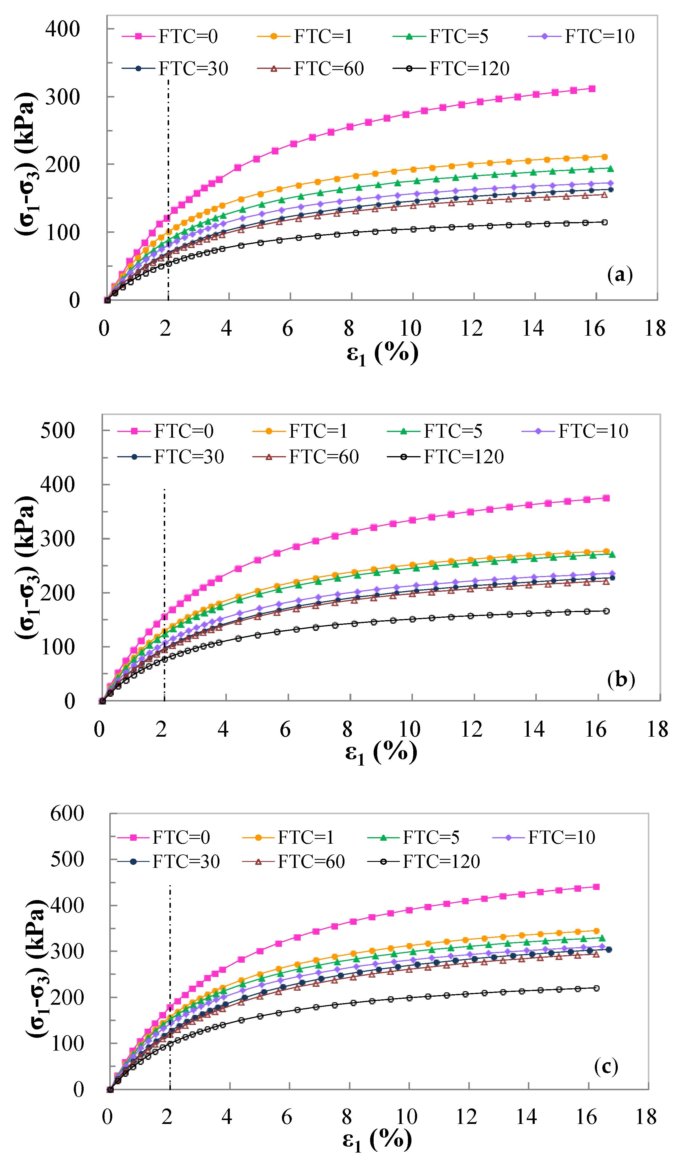
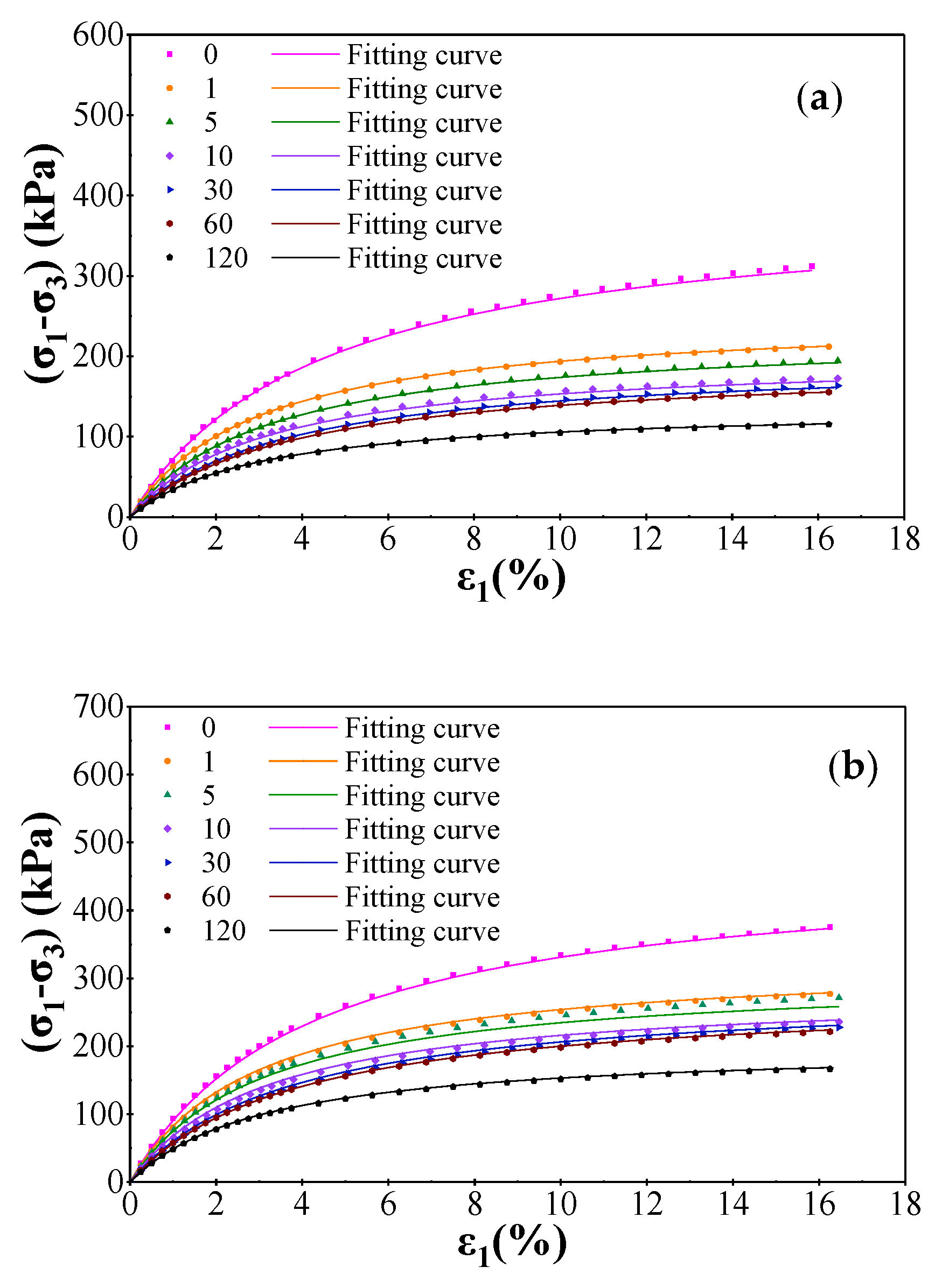
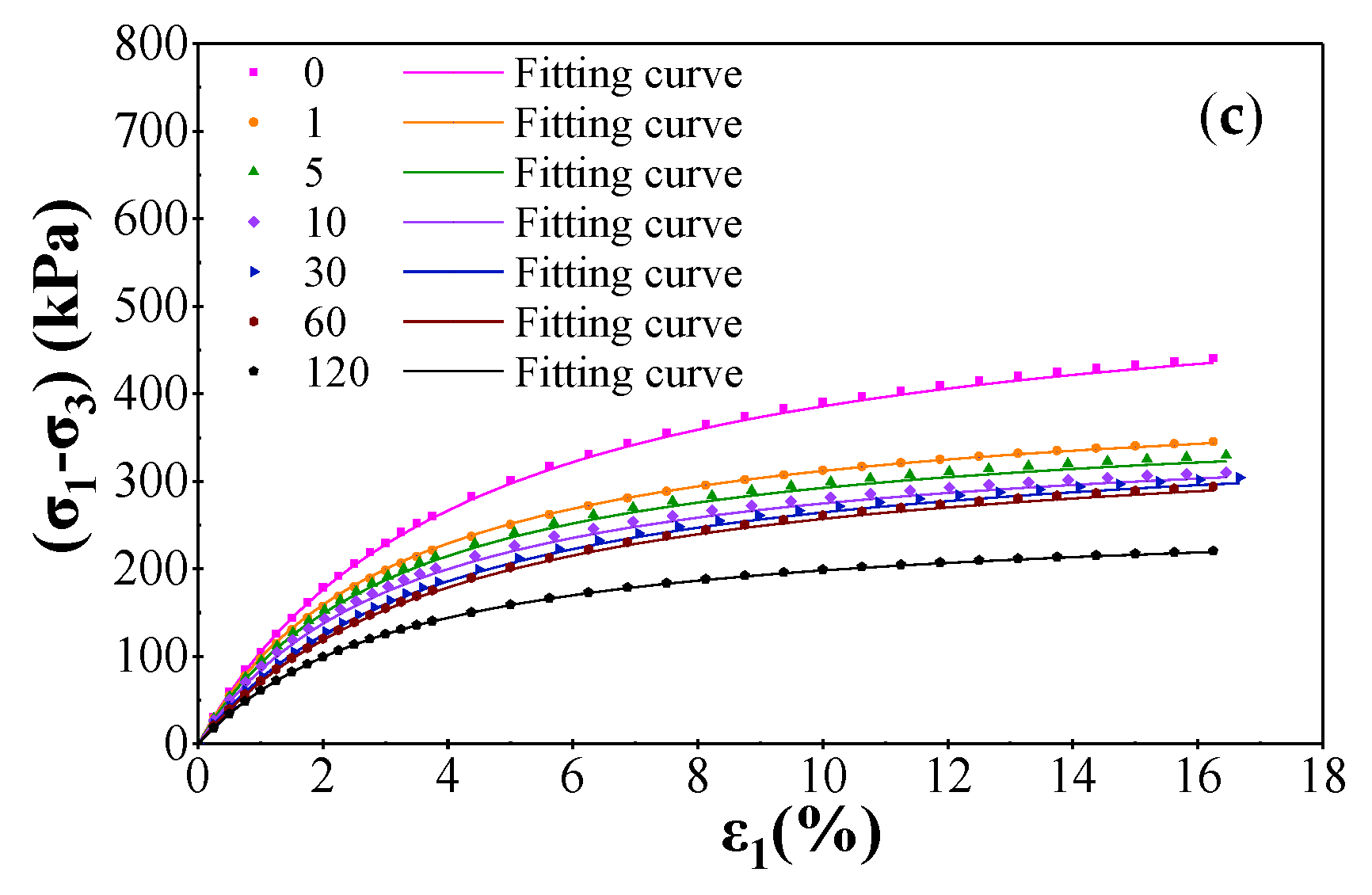
The relational curves between principal-stress deviation (σ₁ − σ₃) and axial strain ε₁ of samples with 0.5% salt content are shown in Figure 1. Because the laws of stress-strain curve affected by FTCs were similar under different S, the stress-strain curve with 0.5% salt content is illustrated here.

As shown in Figure 1, the principal stress deviation (σ₁ − σ₃) had nonlinear growth with the increase of axial strain ε₁. When σ₃ was the same, the (σ₁ − σ₃) -ε₁ curve-variation tendency of the samples with different FTC was similar. All (σ₁ − σ₃) -ε₁ curves were of the strain-hardening type, and the shape of curves was hyperbolic. The stress-strain curve could be divided into three stages: the quasi-elastic stage, the elastic-plastic deformation stage, and the stable stage.

In the repeated process of freezing and thawing, salt expansion, pore water migration, particle breaking and rearranging, and fracture development, gradually changed the force between soil particles, affecting the macromechanical behavior of saline soil [2,28,29]. The initial yield point of the samples decreased with more FTCs (Figure 1). The samples that underwent more FTCs were easier to damage, and their strength was lower.

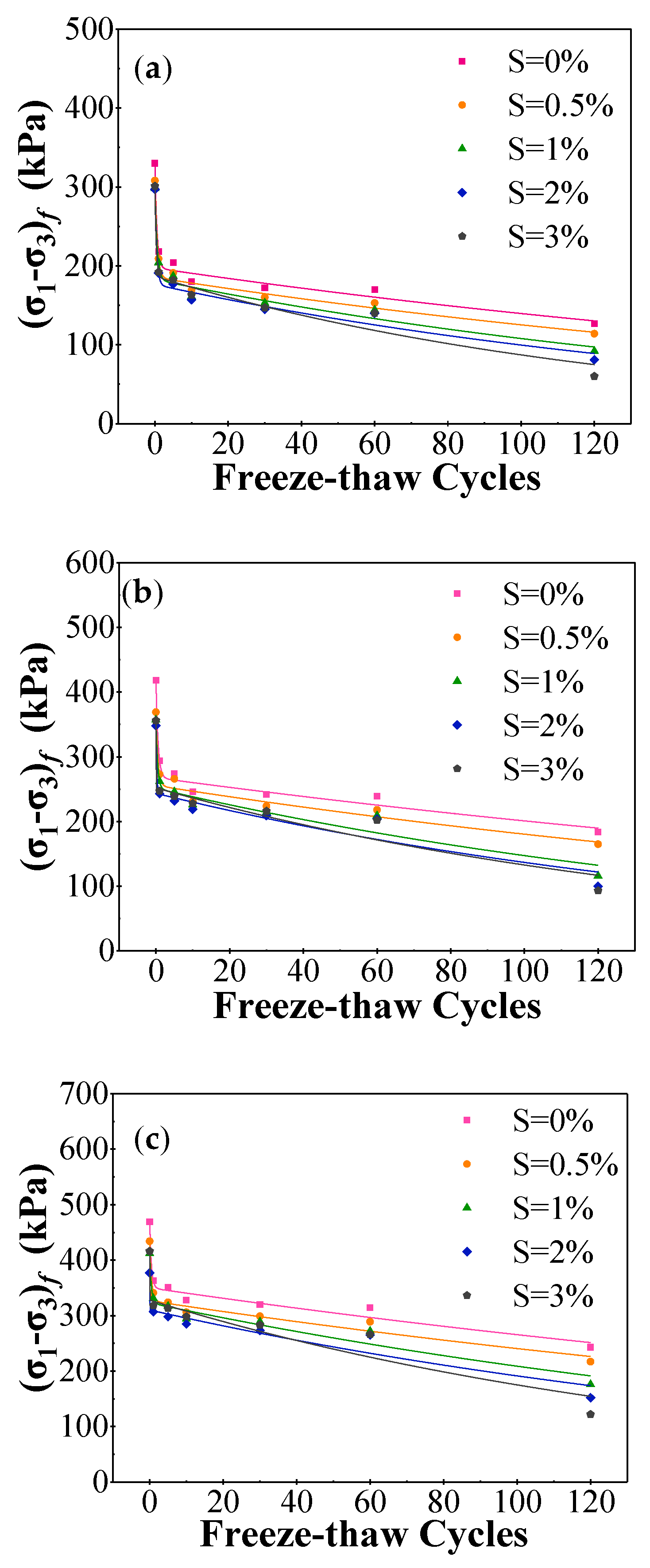
For strain-hardening soil, there is no peak on the stress-strain curves, so principal-stress deviation when the strain value is 15% is usually defined as the shear strength of Nong’an saline soil. It was recorded as (σ₁ − σ₃)_f and called failure principal-stress difference, which is summarized in

Table 2. Failure principal-stress deviation (σ₁ − σ₃)_f of samples.

S (%)	σ3 (kPa)	(σ1 − σ3)f (kPa)
		FTC = 0	FTC = 1	FTC = 5	FTC = 10	FTC = 30	FTC = 60	FTC = 120
0.0	100	330	218	204	180	172	170	127
	200	418	294	274	246	242	239	184
	300	469	363	351	328	320	314	243
0.5	100	308	209	191	169	160	153	114
	200	369	273	266	231	224	218	165
	300	434	341	324	306	299	289	217
1.0	100	298	204	187	161	153	144	92
	200	357	262	246	226	214	209	116
	300	412	331	317	294	289	272	176
2.0	100	297	191	177	157	145	140	81
	200	348	243	232	219	209	204	100
	300	377	307	298	285	273	265	152
3.0	100	301	192	182	163	147	140	60
	200	356	247	239	228	216	202	93
	300	416	318	313	298	283	266	122

. (σ₁ − σ₃)_f of soil varied with FTC change, as shown in Figure 2. The following exponential function was used for curve fitting:

$$y={\mathrm{A}}_1\ast \exp \left({\mathrm{B}}_1\ast x\right)+{\mathrm{C}}_1\ast \exp \left({\mathrm{D}}_1\ast x\right),$$

(1)

where x is the FTC number that the samples underwent, and A₁, B₁, C_1, and D₁ are the fitting parameters. Fitting results are shown in Figure 2, and parameter values are shown in

Table 3. Parameters of exponential function that can reflect the relation between (σ₁ − σ₃)_f and freeze-thaw cycle (FTC).

σ3 (kPa)	S (%)	A1	B1	C1	D1	R2
100	0.0	132.67	−1.82	197.32	−0.0035	0.985
	0.5	122.73	−1.61	185.26	−0.0039	0.989
	1.0	115.46	−1.64	182.53	−0.0053	0.984
	2.0	120.69	−2.04	176.31	−0.0057	0.984
	3.0	114.52	−2.80	186.48	−0.0076	0.974
200	0.0	150.26	−1.71	267.74	−0.0029	0.983
	0.5	113.44	−1.82	255.55	−0.0035	0.974
	1.0	105.63	−2.18	251.37	−0.0053	0.964
	2.0	104.43	−4.84	243.57	−0.0058	0.948
	3.0	103.98	−4.3 × 1011	252.02	−0.0064	0.954
300	0.0	118.93	−2.15	350.07	−0.0028	0.980
	0.5	107.21	−1.95	326.79	−0.0031	0.980
	1.0	88.90	−2.26	232.10	−0.0044	0.965
	2.0	66.83	−7199.2	310.17	−0.0048	0.937
	3.0	87.99	−55,013.5	328.01	−0.0063	0.934

.

The (σ₁ − σ₃)_f of the samples with different S decreased rapidly within 10 cycles, especially about 31.22%–36.42% after the first cycle. At this stage, the structure of Nong’an saline soil was damaged. Then, it slowly declined between 10 and 60 cycles, and it declined faster after samples underwent 120 cycles (24.85%–57.13%). During the first freezing, water in the soil became ice and the volume expanded, which made small particles agglomerate and the aggregates separated from each other. Moreover, pore volume in the soil increased. When the ice melted, aggregate changes and the pore volume in the soil could not recover completely during the thawing process. After the first cycle, the structure of Nong’an saline soil was seriously damaged and its strength decreased rapidly. After 5 and 10 cycles, the micro and small pores in the soil gradually became medium and large pores, large particles or aggregates were separated, and small particles were reunited; finally, the soil entered into a new dynamic and stable equilibrium state [10,30]. Therefore, the decreasing rate of (σ₁ − σ₃)_f was obviously reduced when samples underwent 30 and 60 cycles. However, as the number of FTCs increased, pores in the soil gradually spread into cracks, so soil strength had an accelerated decline after 120 cycles.

The exponential function can reflect the relationship between (σ₁ − σ₃)_f and FTC. Correlation coefficient R² was above 0.93, so this function is suitable to explain the relationship between (σ₁ − σ₃)_f and FTC.

(σ₁ − σ₃)_f increased with confining pressure, which indicated that the latter could inhibit pore-volume changes caused by axial pressure. So, confining pressure can slightly enhance the strength of the samples and have a certain inhibitory effect on deformation and failure [11,31].

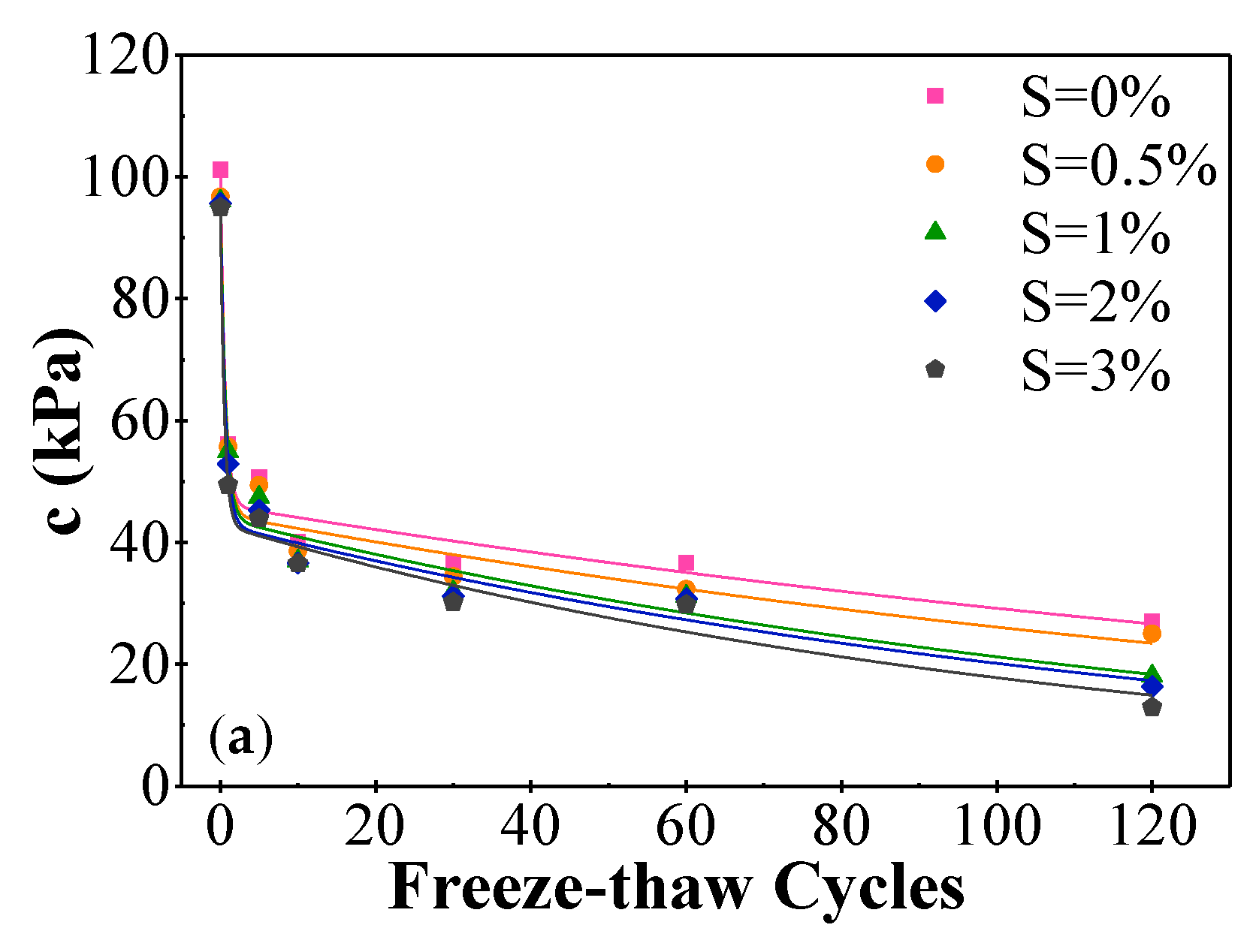
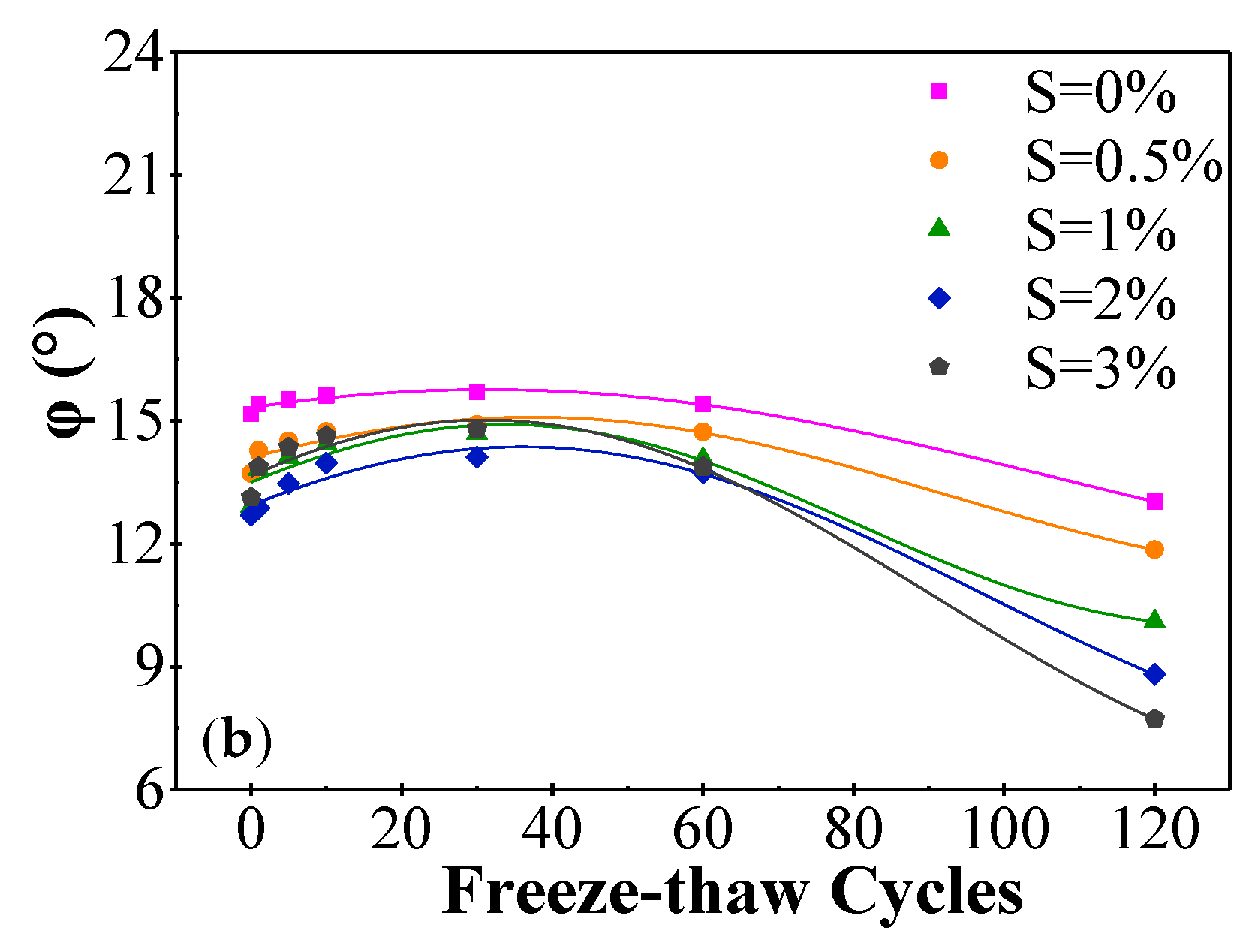
c and the φ are two important indices for evaluating soil’s shear strength that are mainly affected by particle-size composition, arrangement, and cementation [32,33,34]. Recurrent FTC and changes in S change these factors, thus affecting soil c and φ. According to the experiment data, c and φ of the sample could be obtained, as shown in

Table 4. Sample cohesion c and friction angle φ.

Shear Strength	S (%)	FTC = 0	FTC = 1	FTC = 5	FTC = 10	FTC = 30	FTC = 60	FTC = 120
c (kPa)	0.0	101.19	56.09	50.69	40.09	36.78	36.62	27.09
	0.5	96.73	55.67	49.40	38.61	34.43	32.33	25.01
	1.0	96.04	54.96	47.45	36.97	31.96	31.18	18.12
	2.0	95.66	52.87	45.27	36.62	31.22	30.78	16.34
	3.0	94.98	49.42	43.90	36.53	30.18	29.80	12.93
φ (°)	0.0	15.17	15.41	15.52	15.62	15.71	15.41	13.03
	0.5	13.72	14.28	14.51	14.74	14.91	14.73	11.86
	1.0	12.92	13.81	14.11	14.43	14.69	14.07	10.11
	2.0	12.70	12.87	13.47	13.97	14.11	13.74	8.81
	3.0	13.13	13.87	14.35	14.63	14.80	13.88	7.72

. As shown in Figure 3, c and φ were related to FTCs. The exponential function (Equation (1)) could explain the relationship between c and FTC, while the Fourier function could explain the relationship between φ and FTC. The two functions’ parameters are shown in

Table 5. Parameters of exponential and Fourier functions that can reflect relationship between c, φ, and FTC under different S.

S (%)	c (kPa)-FTC					φ (°)-FTC
	A1	B1	C1	D1	R2	A2	B2	C2	D2	R2
0.0	13.58	1.75	1.32	0.021	0.993	55.02	−1.69	46.16	−0.0046	0.983
0.5	1.66	0.91	1.66	0.029	0.962	52.09	−1.52	44.63	−0.0054	0.982
1.0	12.47	1.04	2.21	0.033	0.962	52.00	−1.53	44.03	−0.0073	0.985
2.0	10.80	2.14	2.85	0.026	0.985	52.62	−1.64	43.04	−0.0076	0.988
3.0	10.72	2.93	3.15	0.026	0.986	52.07	−2.02	42.91	−0.0088	0.988

.

The Fourier function is as follows:

$$y={\mathrm{A}}_2+{\mathrm{B}}_2\ast \cos \left({\mathrm{B}}_2\ast x\right)+{\mathrm{C}}_2\ast \sin \left({\mathrm{D}}_2\ast x\right),$$

(2)

where x is the number of FTCs the samples underwent, and A₂, B₂, C_2, and D₂ are the fitting parameters.

According to Figure 3, the exponential function can reflect well the variation regulation of c with FTC. The overall trend of c decreased with FTC number, and c decreased considerably when FTCs varied from 0 to 10, especially when samples underwent the first cycles. After that, decline was slow and c was basically stable at around 30 kPa between 10 and 60 cycles; φ increased when below 30 cycles, and then decreased rapidly after 60 cycles. The Fourier function reflects the law of φ with FTC very well.

4. Determination of Duncan-Chang Model Parameters

As shown in Figure 1, relational curves between principal-stress deviation (σ₁ − σ₃) and axial strain ε₁ of samples are hyperbolic. Therefore, the Duncan-Chang model was suitably applied to analyze the relationship between sample stress and strain [13]. The relationship between model parameters and FTC is discussed below.

Kondner et al. (1963) [13] analyzed the stress-strain curve of soil morphology on the basis of a large number of triaxial shear-test data, and suggested that the hyperbolic function was suitable for simulating the stress-strain relationship of soils:

$${\mathsf{\sigma }}_1-{\mathsf{\sigma }}_3=\frac{{\mathsf{\epsilon }}_1}{\mathrm{a}+{\mathrm{b}\mathsf{\epsilon }}_1},$$

(3)

where a and b are parameters that could be determined by conventional triaxial shear test.

Since dσ₂ = dσ₃ = 0 in the triaxial test, tangent elastic modulus E_t could be obtained by taking the derivative of Equation (3) and eliminating axial strain ε₁:

$${\mathrm{E}}_{\mathrm{t}}=\frac{1}{\mathrm{a}}\left[1-\mathrm{b}\left({\mathsf{\sigma }}_1-{\mathsf{\sigma }}_3\right)\right]={\mathrm{E}}_{\mathrm{i}}\left[1-\frac{\left({\mathsf{\sigma }}_1-{\mathsf{\sigma }}_3\right)}{{\left({\mathsf{\sigma }}_1-{\mathsf{\sigma }}_3\right)}_{ult}}\right],$$

(4)

where E_i is the initial elastic modulus, and (σ₁ − σ₃)_ult is the ultimate principal-stress deviation.

Ultimate principal-stress deviation is difficult to be directly obtained through the test, but failure principal-stress difference is easy to determine. Therefore, in order to obtain the ultimate principal-stress deviation, the failure ratio was defined as follows:

$${\mathrm{R}}_f=\frac{{\left({\mathsf{\sigma }}_1-{\mathsf{\sigma }}_3\right)}_f}{{\left({\mathsf{\sigma }}_1-{\mathsf{\sigma }}_3\right)}_{ult}}.$$

(5)

According to Mohr-Coulomb strength theory:

$${\left({\mathsf{\sigma }}_1-{\mathsf{\sigma }}_3\right)}_f=\frac{2\mathrm{c}\cos \mathsf{\Phi }+2{\mathsf{\sigma }}_3\sin \mathsf{\Phi }}{1-\sin \mathsf{\Phi }}.$$

(6)

We transformed the coordinate system of Equation (3) to get the following equation:

$$\frac{{\mathsf{\epsilon }}_1}{{\mathsf{\sigma }}_1-{\mathsf{\sigma }}_3}=\mathrm{a}+{\mathrm{b}\mathsf{\epsilon }}_1.$$

(7)

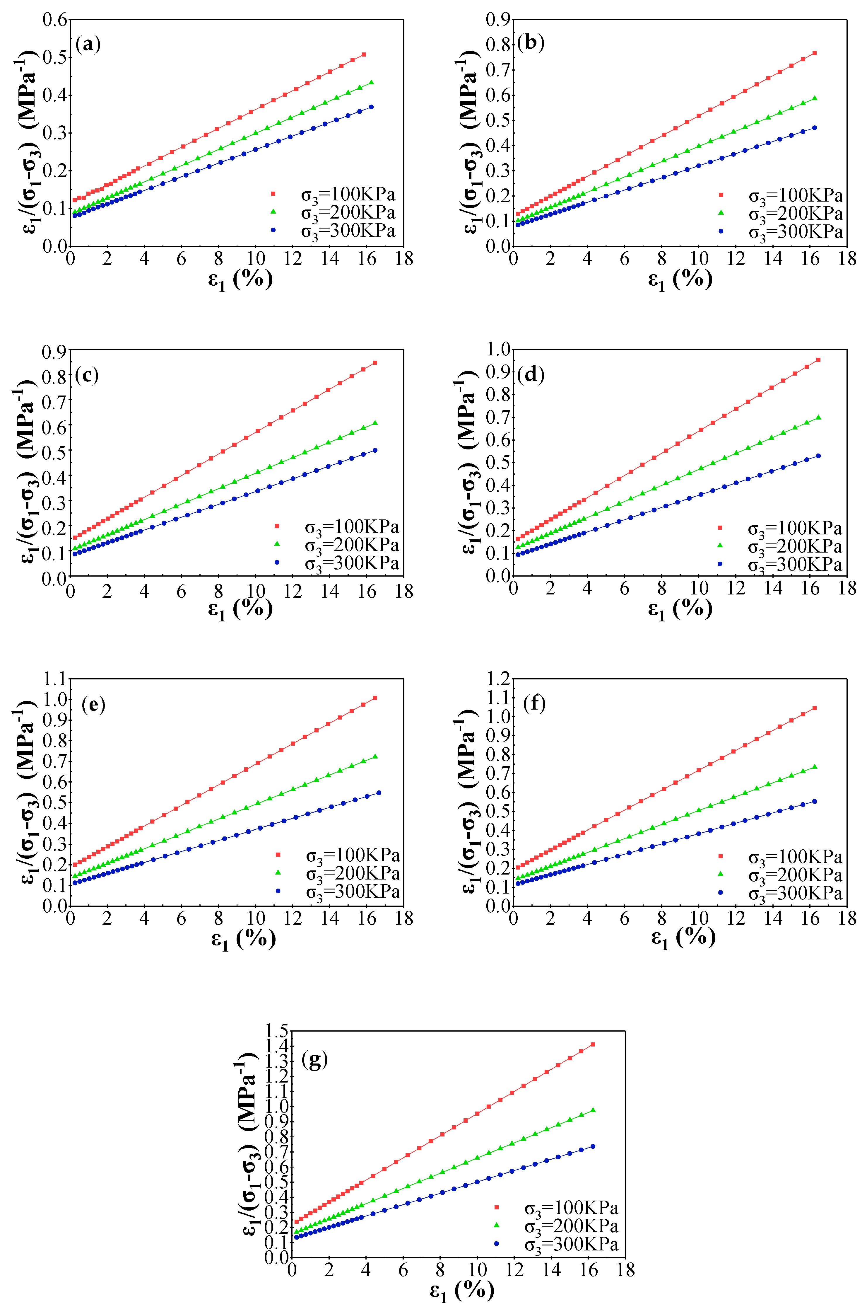
According to Equation (7), triaxial test data are transformed into another coordinate, and curves of ε₁/(σ₁ − σ₃) and ε₁ were drawn in Figure 4. It can be seen from Figure 4 that there was a first-order linear correlation between stress and strain in the ε₁/(σ₁ − σ₃) − ε₁ coordinate. The stress-strain curve of the sample conformed to the hyperbolic function. The y-intercept of the fitting line was parameter a, and the slope was parameter b, as shown in

Table 6. Parameters a and b of curves ε₁/(σ₁ − σ₃) -ε₁ under different conditions.

S (%)	FTC	σ3 = 100 kPa		σ3 = 200 kPa		σ3 = 300 kPa
		a(MPa−1)	b(MPa−1)	a(MPa−1)	b(MPa−1)	a(MPa−1)	b(MPa−1)
0.0	0	0.095	2.390	0.077	1.880	0.065	1.690
	1	0.112	3.840	0.088	2.810	0.074	2.260
	5	0.134	3.990	0.096	3.000	0.079	2.320
	10	0.145	4.600	0.107	3.350	0.086	2.480
	30	0.188	4.980	0.136	3.560	0.106	2.650
	60	0.184	4.670	0.126	3.330	0.102	2.500
	120	0.218	6.440	0.146	4.470	0.123	3.290
0.5	0	0.113	2.490	0.085	2.143	0.076	1.798
	1	0.119	3.990	0.094	3.030	0.079	2.410
	5	0.141	4.290	0.101	3.070	0.081	2.540
	10	0.151	4.880	0.117	3.530	0.087	2.690
	30	0.188	4.980	0.136	3.560	0.106	2.650
	60	0.191	5.260	0.137	3.670	0.112	2.710
	120	0.221	7.330	0.157	5.030	0.126	3.760
1.0	0	0.130	2.491	0.101	2.126	0.079	1.898
	1	0.135	3.980	0.102	3.140	0.083	2.470
	5	0.148	4.350	0.104	3.370	0.084	2.600
	10	0.164	5.100	0.118	3.640	0.088	2.810
	30	0.192	5.250	0.137	3.770	0.114	2.700
	60	0.198	5.620	0.141	3.850	0.117	2.890
	120	0.236	9.280	0.163	7.480	0.128	4.810
2.0	0	0.130	2.506	0.101	2.198	0.081	1.900
	1	0.141	4.270	0.105	3.420	0.084	2.700
	5	0.156	4.610	0.108	3.590	0.085	2.790
	10	0.176	5.180	0.121	3.750	0.091	2.900
	30	0.216	5.480	0.146	3.820	0.124	2.840
	60	0.217	5.690	0.151	3.900	0.128	2.920
	120	0.242	10.800	0.172	8.900	0.131	5.710
3.0	0	0.122	2.506	0.087	2.240	0.078	1.890
	1	0.137	4.300	0.103	3.350	0.083	2.590
	5	0.152	4.480	0.105	3.470	0.082	2.640
	10	0.168	5.020	0.119	3.640	0.085	2.780
	30	0.207	5.430	0.135	3.730	0.111	2.790
	60	0.209	5.760	0.149	3.960	0.127	2.910
	120	0.238	15.100	0.168	9.590	0.129	7.350

. The reciprocal of parameters a and b are E_i and (σ₁ − σ₃)_ult, respectively.

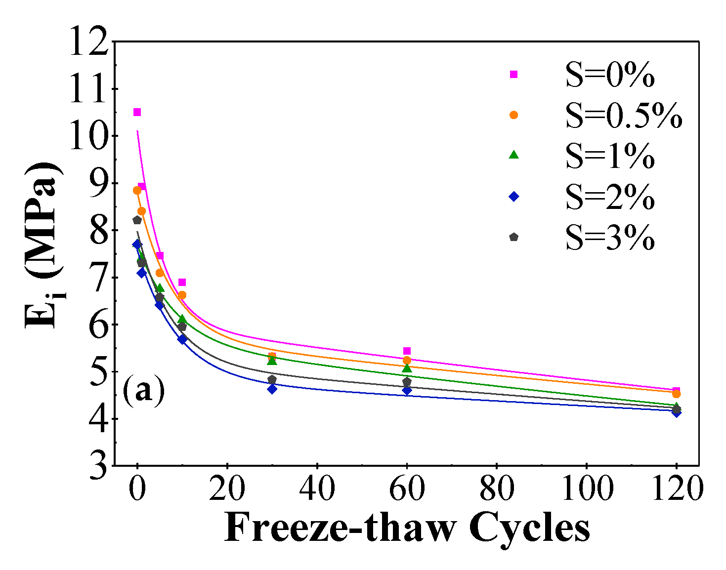
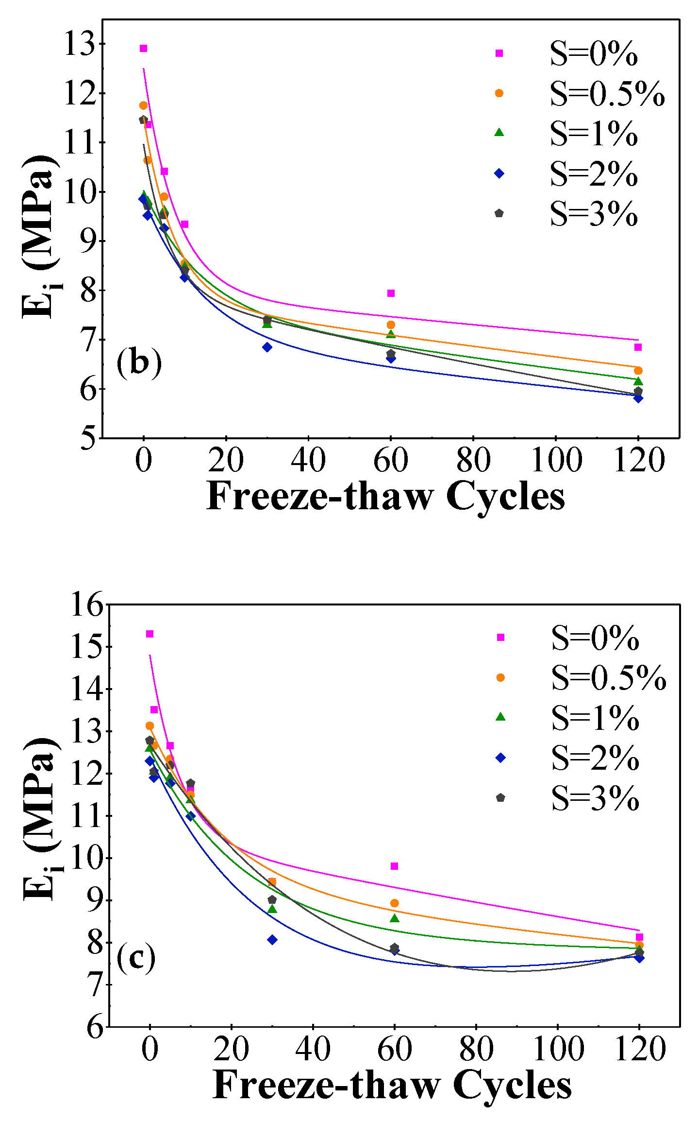
In Figure 5, under different confining pressures, the variation tendencies of initial tangent modulus E_i and FTC were similar, decreasing rapidly below 30 cycles, and then decreasing slowly after 30 cycles. The regression relation of E_i to FTC could be fitted by the exponential function, and fitting parameters are shown in

Table 7. Parameters of exponential functions that can reflect relationship between E_i and FTC under different σ₃ and S.

σ3 (kPa)	S (%)	A1	B1	C1	D1	R2
100	0.0	4.09	−0.19	6.02	−0.0022	0.99996
	0.5	3.07	−0.13	5.73	−0.0019	0.99999
	1.0	2.07	−0.12	5.63	−0.0023	1.00000
	2.0	2.75	−0.11	4.83	−0.0012	0.99999
	3.0	2.80	−0.13	5.17	−0.0017	0.99999
200	0.0	4.54	−0.13	7.97	−0.0011	0.99993
	0.5	3.72	−0.14	7.80	−0.0016	0.99998
	1.0	2.43	−0.07	7.60	−0.0017	0.99998
	2.0	2.89	−0.07	6.99	−0.0015	0.99999
	3.0	3.00	−0.16	7.97	−0.0025	0.99994
300	0.0	4.36	−0.14	10.45	−0.0019	0.99991
	0.5	3.82	−0.05	9.27	−0.0013	0.99998
	1.0	4.61	−0.04	7.96	−0.00001	0.99996
	2.0	6.29	−0.04	6.12	0.0018	0.99995
	3.0	10.35	−0.02	2.33	0.0082	0.99995

.

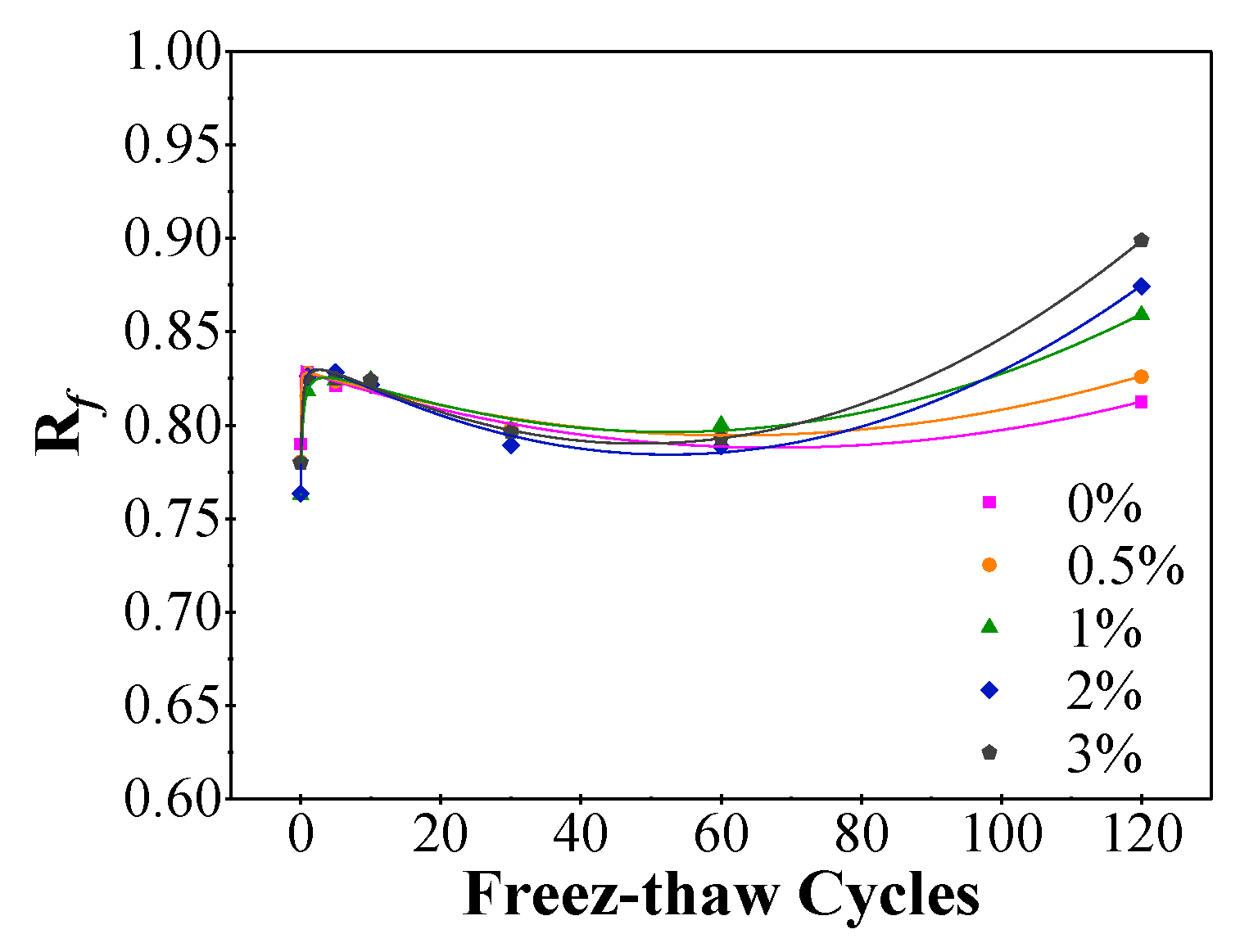
The failure principal-stress deviator (σ₁ − σ₃)_f and limiting principal-stress deviator (σ₁ − σ₃)_ult were determined. According to Equation (5), fracture ratio R_f could be obtained. As shown in Figure 6, R_f increased after the first cycle, and then decreased between five and 60 cycles. After 120 cycles, R_f obviously increased. The following rational function was used for curve fitting:

$$y=\left({\mathrm{A}}_3\ast x^3+{\mathrm{B}}_3\ast x^2+{\mathrm{C}}_3\ast x+\mathrm{D}\right)/\left(x+{\mathrm{E}}_3\right),$$

(8)

where x is the FTC number that the samples underwent, and A₃, B₃, C₃, D₃, and E₃ are fitting parameters. The fitting result is shown in Figure 6, and parameter values are shown in

Table 8. Parameters of rational function that could reflect the relationship between R_f and FTC under different S.

S (%)	A3	B3	C3	D3	E3	R2
0.0	8.99 × 10−6	−0.0012	0.83	−0.01	−0.01	1
0.5	9.33 × 10−6	−0.0012	0.83	0.15	0.18	1
1.0	1.40 × 10−5	−0.0015	0.84	0.22	0.28	1
2.0	2.00 × 10−5	−0.0021	0.84	0.14	0.18	1
3.0	2.13 × 10−5	−0.0021	0.84	0.22	0.29	1

.

According to Janbu’s suggestion, initial tangent modulus E_i is related to σ₃, and its empirical relationship is as follows:

$${\mathrm{E}}_{\mathrm{i}}={\mathrm{KP}}_{\mathrm{a}}{\left(\frac{{\mathsf{\sigma }}_3}{{\mathrm{P}}_{\mathrm{a}}}\right)}^{\mathrm{N}},$$

(9)

where K and N are material constant and P_a = 101.4 kPa is the standard atmospheric pressure.

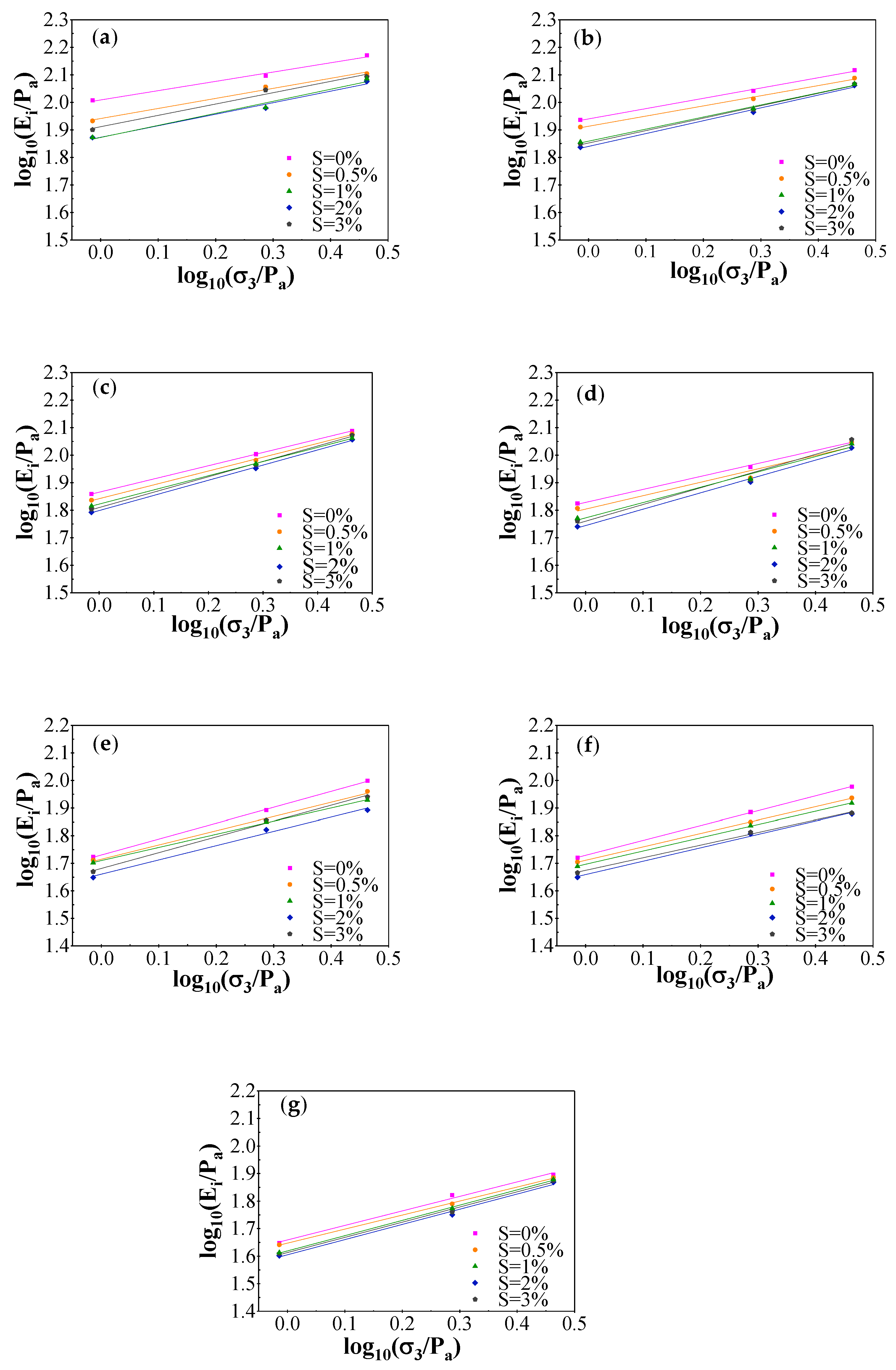
We drew the diagram of log₁₀(σ₃/P_a) and log₁₀ (E_i/P_a), as shown in Figure 7. According to the relationship between log₁₀(σ₃/P_a) and log₁₀(E_i/P_a), the y-intercept and slope of the fitting line were log₁₀(K) and N, respectively, so material constants K and N were obtained, as shown in

Table 9. Values of material constants K and N.

S (%)	Parameters	FTC = 0	FTC = 1	FTC = 5	FTC = 10	FTC = 30	FTC = 60	FTC = 120
0.0	K	102.03	87.10	73.45	67.45	51.88	53.52	45.61
	N	0.34	0.37	0.48	0.47	0.52	0.54	0.53
0.5	K	87.30	81.85	69.50	63.68	51.88	51.44	44.40
	N	0.37	0.37	0.50	0.49	0.52	0.49	0.51
1.0	K	74.56	72.28	66.37	59.16	51.29	49.75	41.60
	N	0.44	0.44	0.52	0.56	0.48	0.48	0.56
2.0	K	74.66	69.18	62.95	55.46	45.81	45.64	40.28
	N	0.42	0.47	0.55	0.59	0.52	0.49	0.55
3.0	K	81.58	71.12	64.57	57.54	48.08	47.29	41.03
	N	0.41	0.45	0.56	0.61	0.57	0.46	0.55

.

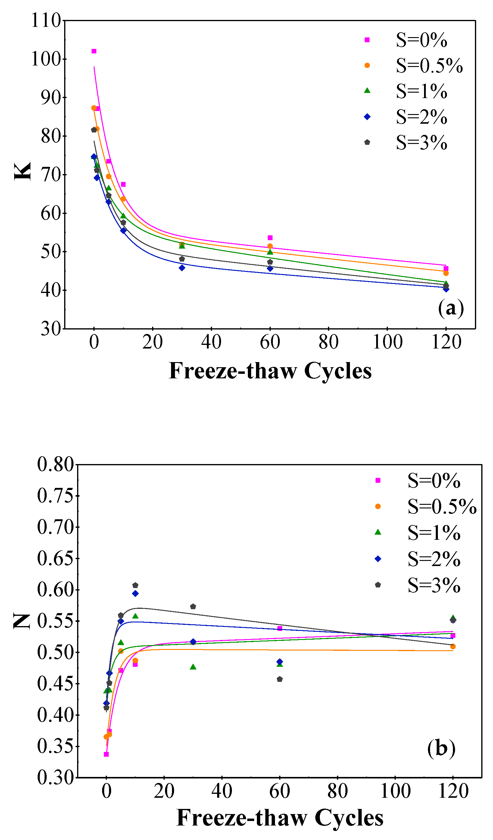
With the increase of FTC, the change rule of material constant K rapidly decreased below 30 cycles, and then slowly decreased after 60 cycles. The regulation of N increased below 10 cycles, and then decreased between 10 and 60 cycles; it then increased after 120 cycles. The regression relation of K-FTC and N-FTC could be fitted by the exponential function; parameters of this function are shown in

Table 10. Parameters of exponential functions that can reflect the relationship of K and N to FTC under different S.

S (%)	K					N
	A1	B1	C1	D1	R2	A1	B1	C1	D1	R2
0.0	42.01	−0.15	56.04	−0.0016	0.9992	−0.17	−0.24	0.51	0.00034	0.999
0.5	31.10	−0.14	55.48	−0.0018	0.9997	−0.16	−0.34	0.51	−0.00004	0.999
1.0	19.79	−0.14	55.65	−0.0023	0.9998	−0.08	−0.46	0.51	0.00036	0.999
2.0	27.38	−0.15	51.43	−0.0018	0.9997	−0.14	−0.56	0.55	−0.00046	0.999
3.0	25.94	−0.12	48.27	−0.0014	0.9998	−0.17	−0.42	0.58	−0.00102	0.999

. And the fitting result is shown in Figure 8.

Stress level S_L is defined as the ratio of actual principal-stress difference (σ₁ − σ₃) to failure principal-stress difference (σ₁ − σ₃)_f:

$${\mathrm{S}}_{\mathrm{L}}=\frac{\left({\mathsf{\sigma }}_1-{\mathsf{\sigma }}_3\right)}{{\left({\mathsf{\sigma }}_1-{\mathsf{\sigma }}_3\right)}_f},$$

(10)

By substituting Equations (5), (6), (9) and (10) into Equation (4), we can get the following formula:

$${\mathrm{E}}_{\mathrm{t}}={\mathrm{KP}}_{\mathrm{a}}{\left(\frac{{\mathsf{\sigma }}_3}{{\mathrm{P}}_{\mathrm{a}}}\right)}^{\mathrm{N}}{\left[1-\frac{{\mathrm{R}}_{\mathrm{f}}\left(1-\sin \mathsf{\Phi }\right)\left({\mathsf{\sigma }}_1-{\mathsf{\sigma }}_3\right)}{2\mathrm{c}\cos \mathsf{\Phi }+2{\mathsf{\sigma }}_3\sin \mathsf{\Phi }}\right]}^2.$$

(11)

Simplified:

$${\mathrm{E}}_{\mathrm{t}}={\mathrm{E}}_{\mathrm{i}}{\left(1-{\mathrm{R}}_f{\mathrm{S}}_{\mathrm{L}}\right)}^2.$$

(12)

In conclusion, the experience formula of the five material constants contained in the tangent deformation modulus of the Duncan-Chang model were established, so the variation regular of the tangent deformation modulus with the FTC could be determined by unconsolidated undrained tests.

In the triaxial unconsolidated, undrained shear tests, no volumetric strain occurred in the samples. So, material constants G, F, and D that calculate tangential Poisson’s ratio in the E-μmodel (initial tangent modulus - tangent Poisson’s ratio model) could not be obtained, nor could the K_b and m of the E-B model (initial tangent modulus -bulk modulus model) be obtained. According to the generalized Hooke’s law, the value of μ_t was 0.5 when the sample strain was 0. In order to ensure the stability of numerical calculation, Poisson’s ratio is usually 0.49 [35].

5. Model Validation

By using Equations (5), (6) and (9), we could calculate hyperbolic model parameters a and b. According to Equation (6), the calculated results could be drawn in a stress-strain diagram, and we compared them with the experimental stress-strain curves. As shown in Figure 9, stress-strain curves that were determined by the modified Duncan-Chang model were, considering the FTC, basically close to the experiment stress-strain curves; the simulation effect was better in the stage when the strain was small and there was nearly elastic deformation. When the strain increased to 4%, there was a difference between some simulated and experimental curves. On the whole, it was reasonable to use this model to simulate the stress-strain curve of Nong’an saline soil affected by FTCs under the condition of an unconsolidated, undrained triaxial test.

6. Conclusions

In this paper, Nong’an saline soil from Western Jilin was taken as the research object. Through unconsolidated, undrained triaxial shear tests, the relationship between the mechanical properties of Nong’an saline soil and freeze-thaw cycles was studied, and a modified Duncan-Zhang constitutive model was established.

The stress-strain curves of the remolded saline soil were strain-hardening. There was linear elastic deformation in the initial loading stage, and it entered into the elastic-plastic deformation stage when strain reached 2%. With the increase of FTCs, (σ₁ − σ₃)_f and c both decreased, rapidly decreasing after the first cycle and becoming stable between 30 and 60 cycles. φ increased at first, and then decreased. Using the exponential function could explain the relationship of (σ₁ − σ₃)_f and c to FTC, and φ to FTC could be fitted by the Fourier function. Fitting results showed that the two functions reflected their variation rule well.

On the basis of Duncan-Chang model theory and regression analysis of the experimental data, a modified Duncan-Chang model was established for Nong’an saline soil, and the relationships of parameters E_i, K, N, and R_f to FTCs were analyzed. The analysis results indicated that E_i and K decreased rapidly at first and then became stable. R_f and N increased at first and then decreased. After 120 cycles, R_f and N all obviously increased. The relationships of E_i, K, and N to FTC could be explained by the exponential function, and the relationship of R_f to FTC could be explained by the rational function.

The rationality of the model was verified by comparing the simulation and experiment curves. It was found that, in the low-strain elastic-deformation stage, the model simulation results were consistent with the experiment results. When the strain was higher than 4%, there was little difference between simulated and experimental curves. Therefore, the Duncan-Chang model could well reflect the stress-strain relationship of the remolded Nong’an saline soil as a whole.