Control Strategy to Regulate Voltage and Share Reactive Power Using Variable Virtual Impedance for a Microgrid

Abstract

This paper presents a control strategy to regulate voltage and share reactive power from distributed generators in a microgrid when electric vehicles (EVs) are connected and disconnected at different nodes and times. The control strategy considers fixed and variable virtual impedances created in the microgrid (MG) when loads change (EVs are connected or disconnected). Fixed virtual impedance is related to the distance from each house to the power inverter and is used as an input of the primary control. Variable virtual impedance is associated with the distance from each EV to the power inverter and is also used as an input of the primary control. Thus, the control of the inverter seeks to regulate the voltage where the EVs create variations in the network. The results show that the control strategy regulates well the voltage of different nodes, and the reactive power is distributed to renewable generators based on the distance from the loads to the inverters. By considering the fixed and variable virtual impedances in the primary control, voltage can be regulated, assuming various consumptions of EVs in the network. This result is promising for reactive power control and sharing for each distributed generator (DG) in a microgrid where a great number of EVs affect the operation.

1. Introduction

Private vehicles are responsible for most of the total transport energy consumption and associated pollutants [1]. Therefore, electric vehicles (EVs) provide a better future by not emitting carbon dioxide (CO₂), carbon monoxide (CO), nitrogen oxides (NOx), unburned hydrocarbons (UHCs), lead compounds, sulfur dioxide, and solid particles to the environment, making it a very promising option for transportation [2]. However, the use of EVs requires the periodic charging of batteries, and autonomy must be provided by considering different charging stations operating as nodes in a network that combines the variable loads of home appliances and EVs. Thus, the massive inclusion of EVs will bring issues to the network infrastructure due to branch limits, voltage regulation, and power losses.

A good solution for this problem is the microgrid (MG), which combines several renewable generation units, loads, and storage systems [3] to help mitigate the effects of different EVs charging in the network. Thus, houses and buildings could provide small power vehicle stations with distributed generators (DGs) that can supply this variable load in different nodes. The microgrid concept has been introduced as a very effective technology that integrates renewable energy sources [4] and operates either connected to a main network or in isolation [5]. Transport electrification presents several challenges for the smart grid, such as energy quality, reliability, and control [6].

There are three emerging concepts of EVs connected to the network: vehicle-to-home (V2H), vehicle-to-vehicle (V2V), and vehicle-to-power grid (V2G) [7]. V2H refers to the exchange of energy between the EV battery and the domestic power grid, where batteries can function as the power generator to provide the backup power to the electric home [8]. V2V refers to the local exchange between EVs that can charge or discharge battery power between them. V2G uses the power of the local EV community and exchanges it to the power grid through control [9].

Unidirectional V2G is a technology that controls the battery charging speed of EVs in a single direction of power flow between the EV and the network [10,11]. One advantage of unidirectional V2G technology is that it is not costly to add the simple controller to manage the charge rate. Unidirectional V2G can provide auxiliary services to the power grid, such as power grid regulation and load reservation [12].

Some papers report trends in the concept of EVs, as well as the key technologies in the development of electric mobility from 2002 to 2012, in three different regions of the world. Some consider different stages in the development of EVs [13]. Original data derived from 257 subject experts surveyed in Denmark, Finland, Iceland, Norway, and Sweden have also been obtained that investigate different expectations and visions associated with a low-carbon form of transport, electric mobility, including the vehicle-to-network scheme [14].

However, in the field of energy systems, there are several new paradigms for the power grid that attempt to address several problems [15,16,17]. The current EV industry has encountered many technical issues with the connection of EVs to the power grid. For example, charging vehicles introduces negative impacts on the power grid. The smart grid concept was introduced to consider electric transportation, which has modernized the power system with additional communication functions [18,19]. EV manufacturing technology could provide an opportunity to implement energy stores [20]. The penetration of plug-in electric and hybrid EVs will increase significantly in the coming years. The insertion of EVs in homes will facilitate the use of renewable sources and possibly generate economic benefits for users, but will also present some challenges, such as those regarding how the penetration of EVs affects the power quality of existing electricity networks [11].

Recently, the development of the smart grid concept in power grids has advanced the role of EVs [21]. A control concept for distribution networks with EVs and distributed energy resources has been previously presented. An analysis of the control strategies, market models, and characteristics of existing EVs was performed to take into account the main drawbacks of existing solutions and a new concept of distributed control for the management of the energy system [22]. Another document proposes an allocation planning method for EVs in a multi-agent-based microgrid [23]. A new scheme to provide the necessary primary reserve for EVs by controlling multiple agents of each vehicle is proposed in [24], and a new methodology to determine the optimal EV load–discharge strategy based on the uncertainty of the voltage drop is proposed in [25].

The consulted references show that previous works have focused on active and reactive power control, but few have considered virtual impedance as part of the solution. However, they have not worked on using variable virtual impedance to share the reactive power in a microgrid that considers the distances to the connection of EVs. The objective of this paper is to show reactive power sharing and voltage regulation in a microgrid using the concept of variable virtual impedance related to the line distance between the inverter and the consumption of EVs charging in the power grid. Therefore, the contributions in this article are as follows. Variable virtual impedances are calculated from each inverter to the possible vehicle connection and disconnection point; a voltage control is applied based on the line distance to the EVs connected; and reactive power sharing from distributed generation is achieved to compensate for the nodes in a network once some variations in the loads are presented.

The rest of the document is organized as follows. Section 2 explains the new control strategy to share reactive power after each load variation. Section 3 presents the formulation for the small-signal stability analysis applied to the control strategy. Section 4 shows the results of simulations performed with the software MATLAB-Simulink. Finally, Section 5 presents conclusions and future work.

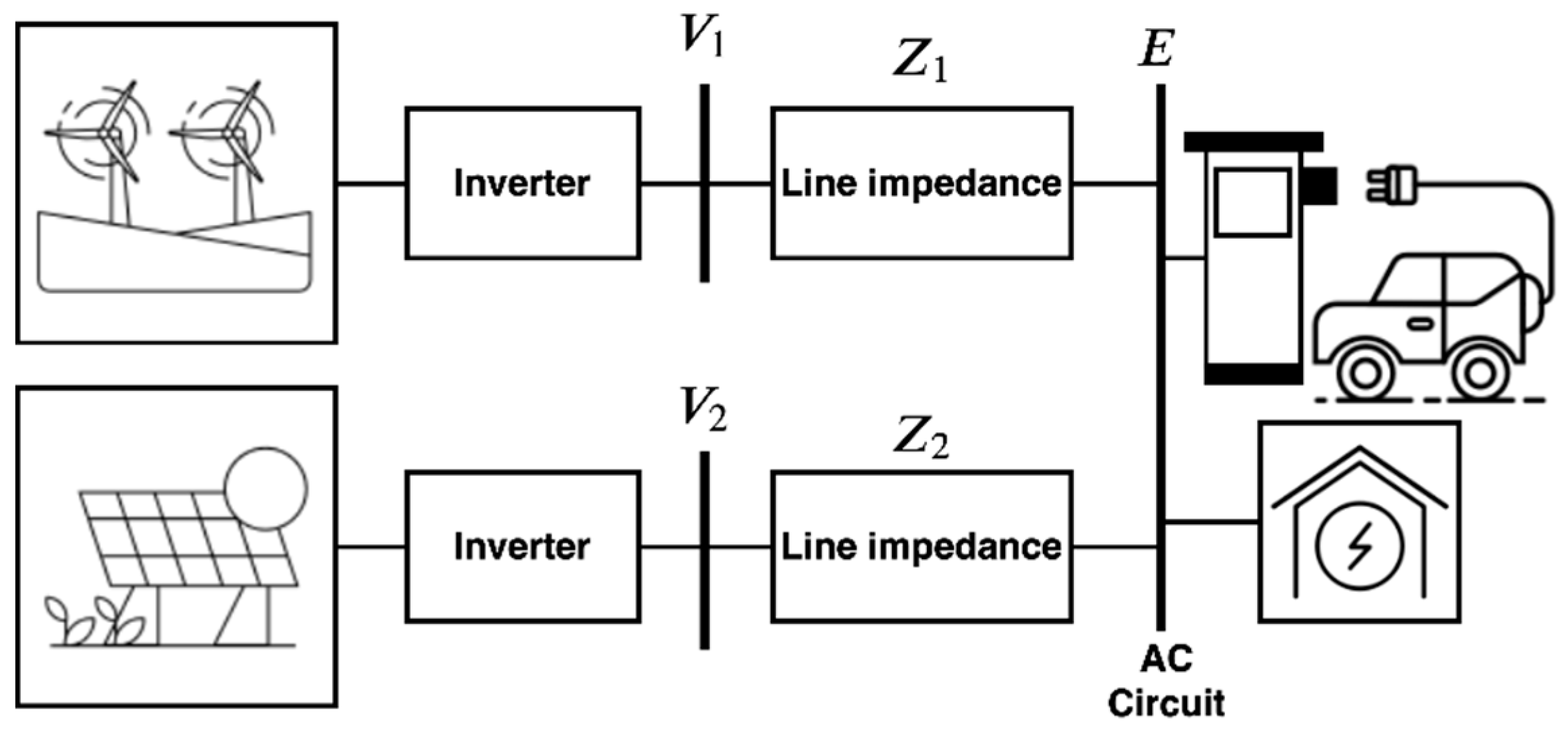
2. Control Method

Droop control P–ω and droop control Q–V have been successfully applied to microgrids [26]. These methods are simple but not very effective when the load changes in different nodes in the microgrid. Therefore, this paper proposes a very useful control strategy for this type of problem. Figure 1 shows the diagram of a single EV and a house connected to a network that uses renewable energies and power inverters.

The active and reactive power transferred from the inverter to the load are given by Equations (1) and (2). These equations express, respectively, the active and reactive power that is lost through the inductive reactance associated with transmission lines. Herein, the term δ represents the phase angle between the voltage generated by the inverters (V) and the voltage of the AC bus $\left(E\right)$. Furthermore, the impedance $Z=R+jX$ has an angle $\theta$ that can be defined as $R=Z\cos \theta$ and $X=Z\sin \theta$:

$$P=\frac{1}{R^2+X^2}\left(R{E}^2-REV\cos \delta +XEV\sin \delta \right),$$

(1)

$$Q=\frac{1}{R^2+X^2}\left(X{E}^2-XEV\cos \delta -REV\sin \delta \right).$$

(2)

A control strategy with virtual impedances is proposed as a method to control the reactive power of the microgrid, considering connections and disconnections of EVs. Figure 2 shows a detailed configuration of a DG unit using the proposed control strategy. The P–ω controller is adopted to regulate the frequency and to achieve accurate reactive power sharing by using virtual impedance.

The controller used with the electrical circuit starts by measuring the current in the inductance of the filter $i_{abc},$ the output voltage $V_{abc}$, and the zero-sequence current $i_{0abc}$. Using the Park transform method, the three previous values are transformed to obtain the $dq$ values, such as $i_{dq},$ $V_{dq},$ and $i_{0dq}$. The active power P is calculated by using the output voltage $V_{dq}$ and the current measured in the output of the system $i_{0dq}$, both in $dq$ coordinates; then, the final signal is passed through the filter and droop controller to obtain θ.

A variable virtual impedance $X_m$, related to the line and load impedances considered from each EV to the inverters, is applied to the control. Then, the total virtual impedance $X_V$ is calculated by summing $X_m$ and a fixed virtual impedance $X_{Vf}$ related to the line and load impedances considered from each house to the inverters, as defined in Equation (3). Reactive power sharing is performed by regulating this total virtual impedance according to the location of EVs in the microgrid.

$$X_V=X_{Vf}+X_m.$$

(3)

Then, the reference voltage $V_{ref}$ is calculated by using the $X_V$ and the $i_{0dq}$. Next, the reference voltage $V_{ref}$ and the output voltage $V_{dq}$ that is measured and transformed to $dq$ coordinates are used to obtain the voltage error, which is then converted to the reference current using the voltage controller.

The voltage control loop uses a PR controller to track the voltage reference value, which is given by the controller. The output of the voltage control gives a reference current that is used to calculate the current error with the $i_{odq}$. The current control loop uses a P controller to adjust the output current that is sent to the pulse width modulation (PWM) to make the inverter obtain the desired voltage response.

3. Small-Signal Stability Analysis

The dynamic model of droop control has been widely discussed [27]. In this section, a small-signal model is derived for the proposed controller in which the total virtual impedance $X_V$ is considered. By considering small disturbances around the equilibrium point defined by ($\Delta \delta e,E,V$), the active power equation can be linearized around this point; thus, the expression shown in Equation (4) is obtained:

$$\Delta P\left(S\right)=\left(\frac{\partial p}{\partial X_V}\right)\Delta X_V\left(S\right)+\left(\frac{\partial p}{\partial \delta }\right)\Delta \delta \left(S\right).$$

(4)

This last equation can be expressed in terms of $k_{px}$ and $k_{p\delta }$ as presented in Equation (5):

$$\Delta P\left(S\right)=k_{px}\Delta X_V\left(S\right)+k_{p\delta }\Delta \delta \left(S\right).$$

(5)

Similarly, the small disturbances around the equilibrium point are defined by ($\Delta \delta e,E,V$), and the reactive power equation can be linearized around this point as expressed in Equation (6):

$$\Delta Q\left(S\right)=\left(\frac{\partial Q}{\partial X_V}\right)\Delta X_V\left(S\right)+\left(\frac{\partial Q}{\partial \delta }\right)\Delta \delta \left(S\right).$$

(6)

This last equation can be expressed in terms of $k_{qx}$ and $k_{q\delta }$, as shown in Equation (7):

$$\Delta Q\left(S\right)=k_{qx}\Delta X_V\left(S\right)+k_{q\delta }\Delta \delta \left(S\right),$$

(7)

where the term $\Delta$ indicates the small-signal deviation of the variable around the equilibrium point, and theses variations are expressed as shown in Equations (8)–(11). Furthermore, the variations of total virtual impedance $\Delta X_V$ in Equation (9) include the changes in the variable virtual impedance $\Delta X_m$ and the changes in the fixed virtual impedance $\Delta X_{Vf}$ (which is considered in this study as zero during the steady-state operation):

$$\Delta W=-k_p\Delta p,$$

(8)

$$\Delta X_V=\Delta X_{Vf }+\Delta X_m,$$

(9)

$$\Delta P=k_{px}\Delta X_V+k_{p\delta }\Delta \delta ,$$

(10)

$$\Delta Q=k_{qx}\Delta X_V+k_{q\delta }\Delta \delta .$$

(11)

The four terms—$k_{px}$, $k_{p\delta },$ $K_{qx},$ and $k_{q\delta }$—are calculated around the equilibrium point, which represents the sensitivity of the power flow with the virtual impedance. Thus, the partial derivative of the active power based on virtual impedance is obtained as shown in Equation (12).

$$k_{px}=\left(\frac{\partial p}{\partial X_V}\right)=\frac{\left(EV\sin \delta \right)\left(R^2+X^2\right)-\left(R{E}^2- REV\cos \delta +XEV\sin \delta \right)\left(2X\right)}{{\left(R^2+X^2\right)}^2}.$$

(12)

The same partial derivative of the active power based on virtual impedance can be expressed as shown in Equation (13):

$$k_{px}=\left(\frac{\partial p}{\partial X_V}\right)=\frac{R^{2}EV\sin \delta -2XR{E}^2}{{\left(R^2+X^2\right)}^2}-\frac{X^{2}EV\sin \delta -2XREV\cos \delta }{{\left(R^2+X^2\right)}^2}.$$

(13)

Now, by considering the partial derivative of the active power with respect to the angle, the term shown in Equation (14) is obtained:

$$k_{p\delta }=\left(\frac{\partial p}{\partial \delta }\right)=\frac{1}{R^2+X^2}\left(REV\sin \delta +XEV\cos \delta \right).$$

(14)

From the partial derivative of the reactive power with respect to the virtual impedance, the expression shown in Equation (15) is obtained:

$$k_{qx}=\left(\frac{\partial Q}{\partial X_V}\right)=\frac{2XREV\sin \delta -E{R}^{2}V\cos \delta }{{\left(R^2+X^2\right)}^2}+\frac{E^2{R}^2-E^2{X}^2+EV{X}^2\cos \delta }{{\left(R^2+X^2\right)}^2}.$$

(15)

Furthermore, from the partial derivative of the reactive power with respect to angle, the following expression shown in Equation (16) is obtained:

$$k_{q\delta }=\left(\frac{\partial Q}{\partial \delta }\right)=\frac{1}{R^2+X^2}\left(XEV\sin \delta -REV\cos \delta \right).$$

(16)

By considering that active and reactive power are commonly measured using a first-order low-pass filter, the cut-off frequency $W_f$ of the active power controller can be linearized around the same point:

$$\Delta W\left(S\right)=\frac{-k_p{W}_f}{S+W_f}\Delta P\left(S\right),$$

(17)

$$\Delta P\left(S\right)=k_{px}\Delta X_V\left(S\right)+k_{p\delta }\Delta \delta \left(S\right).$$

(18)

After replacing $\Delta P\left(S\right)$, as defined in Equations (17) and (18), the following equation is obtained:

$$\Delta W\left(s\right)=\frac{-k_p{W}_f}{S+W_f}\left(k_{px}\Delta X_V\left(S\right)+k_{ps}\Delta \delta \left(S\right)\right).$$

(19)

Thus, the virtual impedance is defined by considering Equation (19):

$$\Delta X_V\left(S\right)=\frac{w_f}{S+w_f}\left[\frac{S\Delta \delta \left(S\right)+k_p{k}_{p\delta }\Delta \delta \left(S\right)}{-k_p{k}_{px}}\right].$$

(20)

After replacing $\Delta X_V$ in Equation (20), Equation (21) is obtained, and considering that $\Delta P\left(S\right)=\frac{S\Delta \delta \left(S\right)}{-k_p}$:

$$\Delta W\left(S\right)=\frac{-k_p{w}_f}{S+w_f}\left\{k_{px}\left[\frac{w_f}{S+w_f}\left(\frac{S\Delta \delta \left(S\right)+k_p{k}_{p\delta }\Delta \delta \left(S\right)}{-k_p{k}_{px}}\right)\right]+k_{p\delta }\Delta \delta \left(S\right)\right\}.$$

(21)

By solving Equation (21), the large expression shown in Equation (22) is obtained.

$$\begin{array}{l}\Delta W\left(S\right)\\ =\frac{-S\Delta \delta \left(S\right)k_{px}{w_f}^2-\Delta \delta \left(S\right)k_{px}{k}_p{k}_{p\delta }{w_f}^2+S\Delta \delta \left(S\right)k_{p\delta }{k}_p{k}_{px}{w}_f+\Delta \delta \left(S\right)k_{p\delta }{k}_p{k}_{px}{w_f}^2}{-S^2{k}_{px}-2S{w}_f{k}_{px}-{w_f}^2{k}_{px}}.\end{array}$$

(22)

After considering that $\Delta W\left(S\right)=S\Delta \delta \left(S\right)$ and replacing this in Equation (22), the expression shown in Equation (23) is obtained.

$$S\Delta \delta \left(S\right)=\frac{-S\Delta \delta \left(S\right)k_{px}{w_f}^2-\Delta \delta \left(S\right)k_{px}{k}_p{k}_{p\delta }{w_f}^2+S\Delta \delta \left(S\right)k_{p\delta }{k}_p{k}_{px}{w}_f+\Delta \delta \left(S\right)k_{p\delta }{k}_p{k}_{px}{w_f}^2}{-S^2{k}_{px}-2S{w}_f{k}_{px}-{w_f}^2{k}_{px}}.$$

(23)

.

Then, after solving Equation (23) and expressing the result in a simplified form, the expression shown in Equation (24) is obtained.

$$S^3\Delta \delta \left(S\right)+2S^2\Delta \delta \left(S\right)w_f+S\Delta \delta \left(S\right)\left({w_f}^2+k_{p\delta }{k}_p{w}_f-{w_f}^2\right)+\Delta \delta \left(S\right)\left(-2 k_p{w_f}^2{k}_{p\delta }\right)=0.$$

(24)

This homogeneous equation describes the free movement of the system for small disturbances around the equilibrium point ($\delta$, E, V), and it can be reduced when considering some constant parameters, as the expression presented in Equation (25):

$$S^3\Delta \delta \left(S\right)+a{S}^2\Delta \delta \left(S\right)+bS\Delta \delta \left(S\right)+c \Delta \delta \left(S\right)=0,$$

(25)

where the parameters $a$, $b$, and $c$ are defined in Equations (26)–(28) as follows.

$$a=2w_f,$$

(26)

$$b=\left({w_f}^2+k_{p\delta }{k}_p{w}_f-{w_f}^2\right),$$

(27)

$$c=\left(-2 k_p{w_f}^2{k}_{p\delta }\right).$$

(28)

Then, the small-signal stability can be studied based on the previous equations. They are implemented in this work for each control system used in the inverters to respond to the load variations at different times and nodes in the network.

4. Results

This section shows the results related to the response of the inverter applied at each generator by considering the variable virtual impedances described in Section 3 to be related to the distance to the connection of the EVs in the microgrid. This strategy allows sharing the reactive power and regulating the voltage in the different nodes. Simulations were performed considering a distribution network case where static loads and EVs are connected.

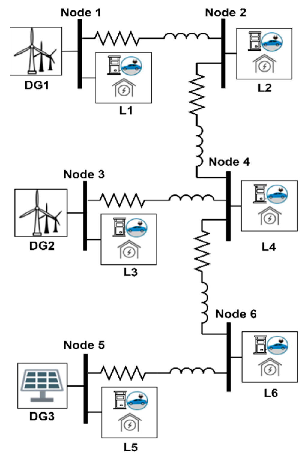
4.1. Distribution Network Case Test

The microgrid used for this research is shown in Figure 3. This network is formed by three distributed generators designed to supply six electrical loads. Each load is composed of fixed loads related to home consumption and variable loads related to connected and disconnected EVs. The power must be delivered considering the impedances of lines 1 to 5, to reach the different loads. Voltage regulation is achieved by using the inverter with the total virtual impedance that considers the lines, fixed loads, and variable loads of the vehicles connected and disconnected.

4.2. Single Electric Vehicle Connection

This test consisted of connecting six EVs at different times and nodes of the microgrid to identify the action of the control strategy with the variable virtual impedance and compare it with the action of the fixed virtual impedance. Thus, the six events are presented in Figure 4 and defined as follows:

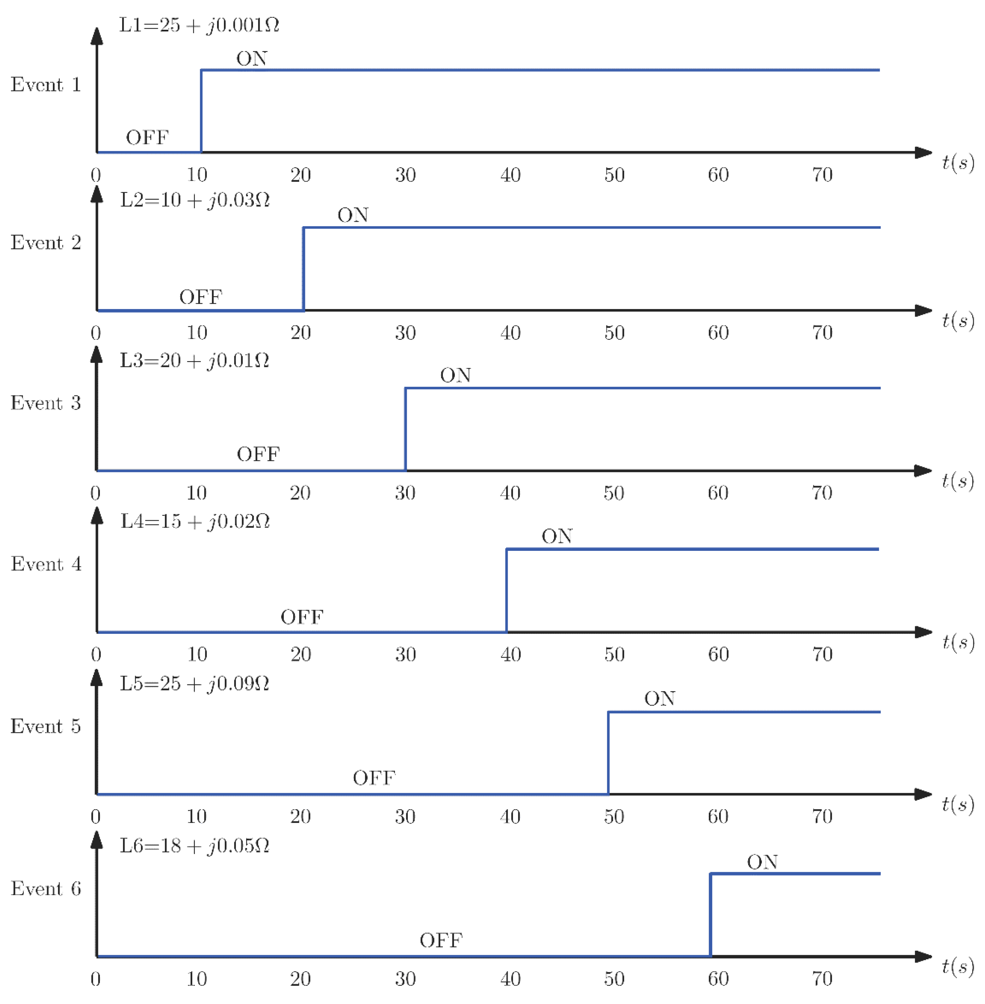
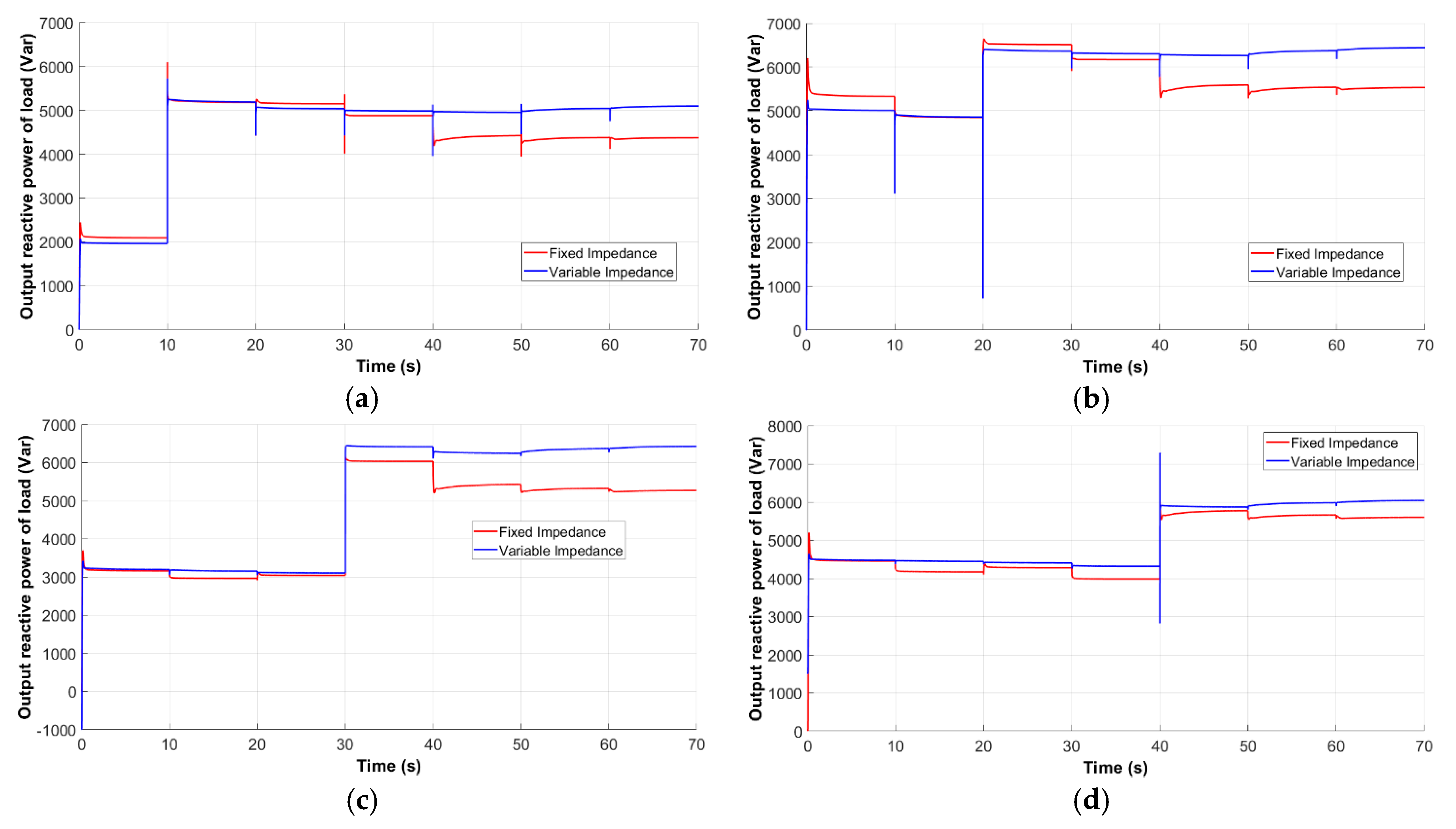
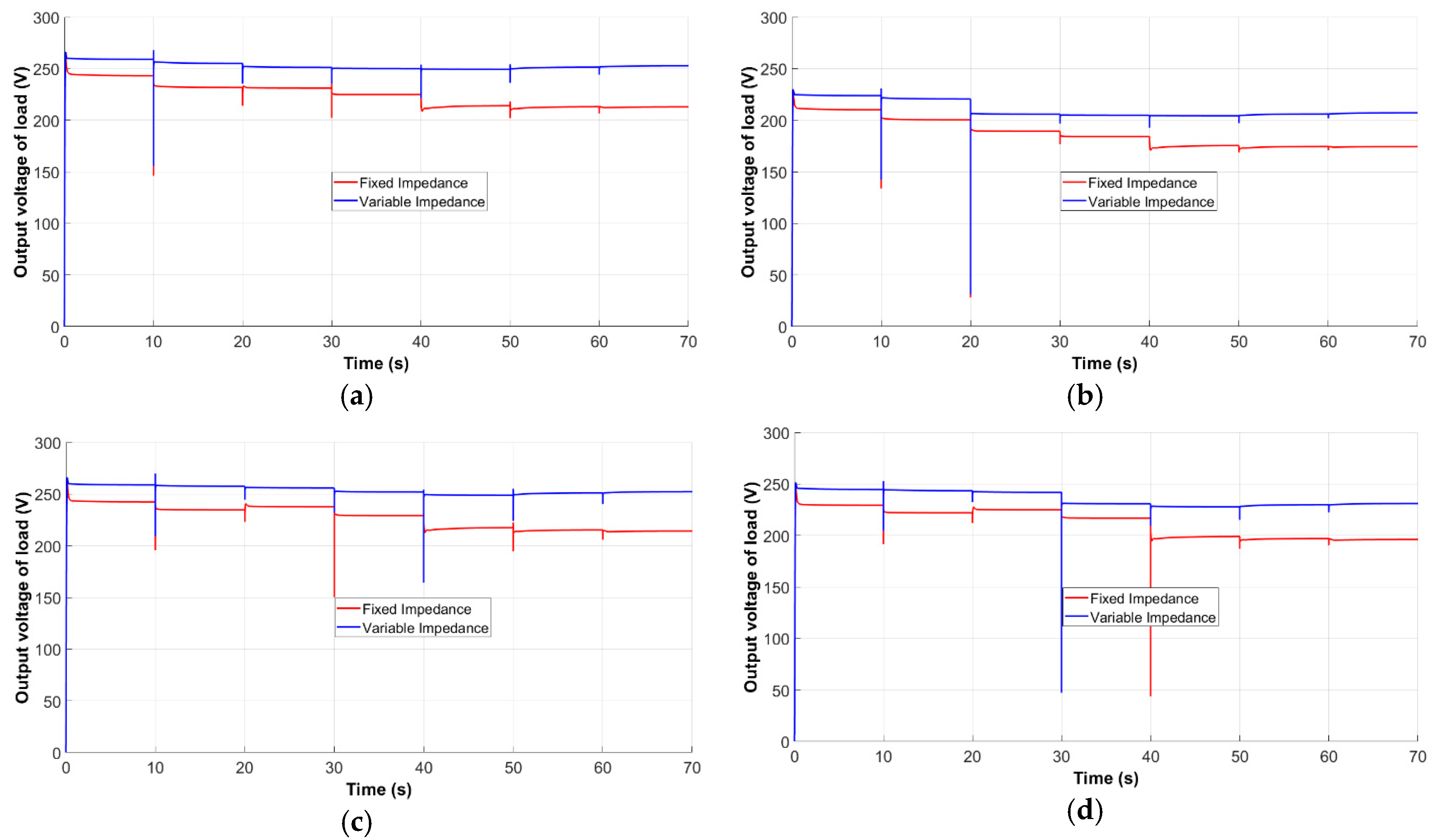
• Event 1: an EV is connected to Node 1 at 10 s, increasing the power consumption of L1 by three times the value of the fixed load (25 + j0.001 Ω).
• Event 2: an EV is connected to Node 2 from 20 s, increasing the power consumption of L2 about three times the value of the fixed load (10 + j0.03 Ω).
• Event 3: from 30 s, an EV is connected to Node 3, increasing the power consumption of L3 by two times the value of the fixed load (20 + j0.01 Ω).
• Event 4: another EV is connected from 40 s to Node 4, increasing the power consumption of L4 by two times the value of the fixed load (15 + j0.02 Ω).
• Event 5: the connection of an EV is presented in Node 5 from 50 to 60 s, increasing the power consumption of L5 by 12 times the value of the fixed load (25 + j0.09 Ω).
• Event 6: this final event considers that an EV is connected from 60 s to Node 6, which generates an additional power consumption of L6 of almost five times the value of the fixed load (18 + j0.05 Ω).

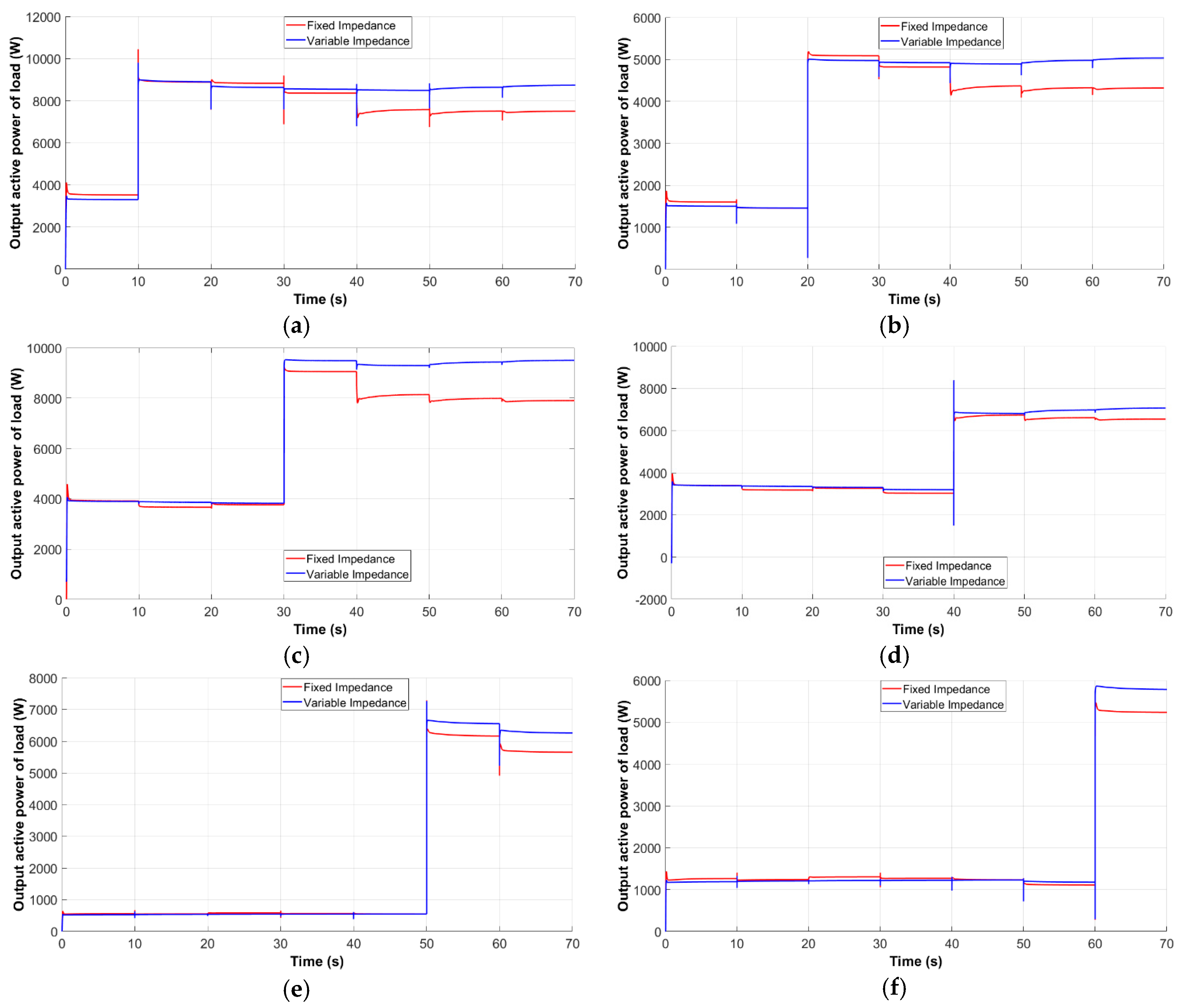
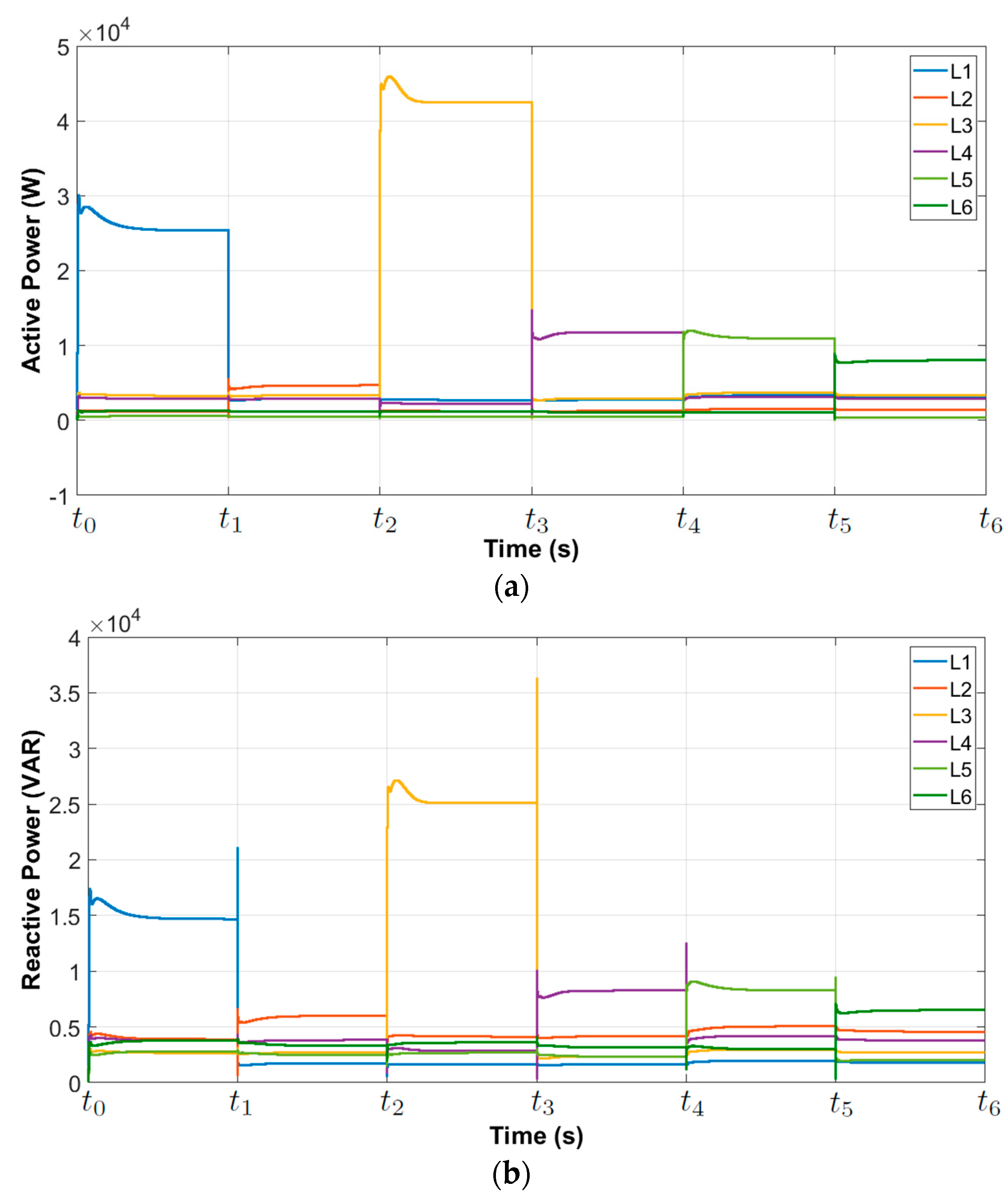
4.2.1. Active and Reactive Power of Loads

Figure 5a–f shows the active power consumption versus time of six loads in the microgrid when EVs are connected at different times and nodes considering the six events presented in the previous subsection. All figures compare the active power supplied to loads L1–L6 when using the control strategy based on fixed and variable virtual impedances.

Hence, Figure 5a presents the active power behavior for Event 1; Figure 5b shows the active power behavior for Event 2; Figure 5c presents the active power behavior for Event 3; Figure 5d shows the active power behavior for Event 4; Figure 5e presents the active power behavior for Event 5; and Figure 5f shows the active power behavior for Event 6. These figures show that the system responds to load variations by delivering active power to each load because of the events that occurred in the microgrid. Both control strategies respond to the changes and share the active power from generation to each load.

During the different periods evaluated, each node presents active power variations that are considered by each inverter according to the control strategy applied. However, the control with the fixed virtual impedance has difficulties in sustaining the power delivered to the load with different power variations presented in the same node plotted and the power variations of other nodes of the microgrid. On the other side, the control with variable virtual impedance is much more effective at maintaining a sustained active power in all the load nodes according to the power variations presented in the same node that are plotted and the power variations of other nodes. Therefore, the proposed control strategy using variable virtual impedance allows maintaining the active power regulated in the different nodes of the microgrid, allowing less power reduction after considering different power variations.

Now, as the reactive power is of great interest in this work, the control strategy must also maintain the power supply to the loads during the power variations. Thus, Figure 6a–f shows the reactive power consumption versus time of the same six loads in the microgrid when the EVs are connected at different times and nodes considering the same six events previously stated. All figures compare the reactive power supplied to loads L1–L6, when using the control strategy based on fixed and variable virtual impedances.

Hence, Figure 6a presents the reactive power supplied to L1 for Event 1; Figure 6b shows the reactive power behavior of L2 for Event 2; Figure 6c presents the reactive power behavior for Event 3; Figure 6d shows the reactive power behavior for Event 4; Figure 6e displays the reactive power behavior for Event 5; and Figure 6f shows the reactive power behavior for Event 6. These figures show that there are variations in the reactive power delivered to each node due to the events that occurred in the microgrid. Both control strategies respond to the changes and share the reactive power from generation to each load.

During the different periods evaluated, each node presents reactive power variations that are considered by each inverter according to the control strategy applied. These six figures show that the reactive power increases to supply loads, but the reactive power is better improved when the variable virtual impedance is used. When the reactive power increases in the load, the fixed virtual impedance allows improving the reactive power demanded to the load node to supply power requirements; however, variations of the different loads in the network reduce the effectiveness of the control and reduce the power supply in the different periods of time. On the other side, the use of the variable virtual impedance follows the variations of the load, increasing the reactive power supply; through the changes of other loads, the reactive power supply is better maintained during the different periods. This shows the advantage of using variable virtual impedance in the controller as it allows improving the reactive power supplied to the loads in better conditions that that supplied by using a fixed virtual impedance.

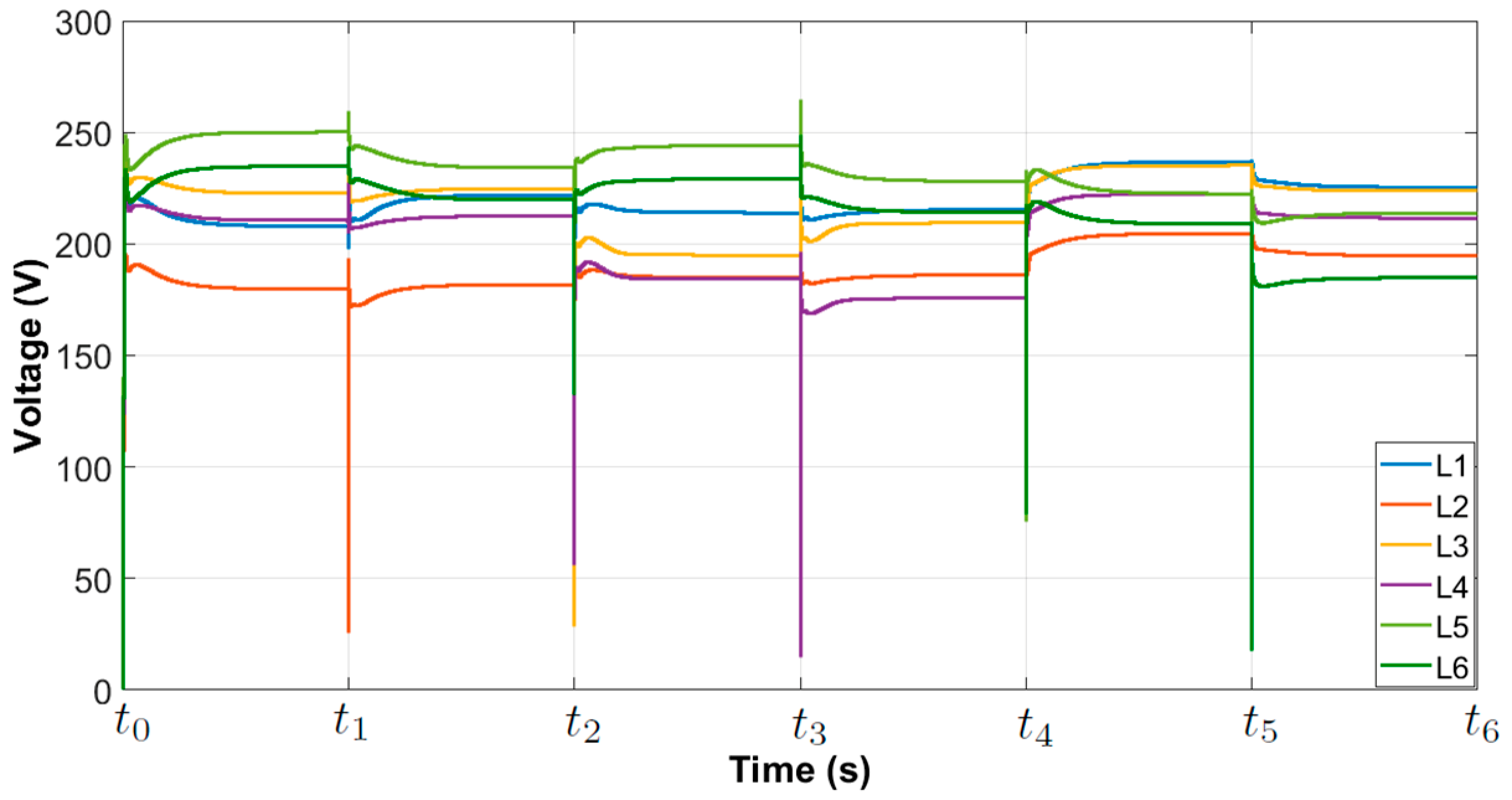
4.2.2. Voltage in Loads

Figure 7a–f shows the voltage behavior in the six nodes of the microgrid when EVs are connected to the network according to the events previously defined. All figures compare the voltage regulated in Nodes 1–6, using the control strategy based on fixed and variable virtual impedances.

Hence, Figure 7a presents the voltage behavior in Node 1 for Event 1; Figure 7b shows the voltage behavior in Node 2 for Event 2; Figure 7c presents the voltage behavior in Node 3 for Event 3; Figure 7d shows the voltage behavior in Node 4 for Event 4; Figure 7e displays the voltage behavior in Node 5 for Event 5; and Figure 7f shows the voltage behavior in Node 6 for Event 6. These figures show that the voltages change in each node according to the events that occurred in the microgrid. Both control strategies respond to regulate well the voltages of each node and maintain them instead of the different power variations presented in the electrical network.

These results show that at the beginning of the EV connection, the voltage of the node tends to drop sharply, but immediately, the control strategy recovers the voltage close to the original value while the EV is charging. Therefore, the control strategy applied with variable virtual impedance maintains a stable voltage value during the different load variation periods when the EVs are connected. On the other side, when the fixed virtual impedance is used, the voltage drops further than the proposed method. The results show that the variable virtual impedance tries to maintain voltage higher than that obtained with fixed virtual impedance, and this means the proposed control strategy is better for improving voltages at different nodes after the events tested.

4.2.3. Responses of DGs

Figure 8 shows the behavior of the power supplied by each DG connected to the microgrid after the six events tested for single EV connection. Figure 8a shows the active power supply, and Figure 8b shows the response of reactive power supply with the strategy control applied with variable virtual impedance. This test allows identifying the distribution of the active and reactive power supplied among generators in the microgrid.

Figure 8 shows that active power increases with the connection of each EV to the different nodes, and each generator stabilizes as quickly as possible to deliver adequate reactive power to the various connections of EVs. In the two first events (10 s and 20 s), it is observed that DG 1 is the one that responds more sharply to the change of load, because it is closer to the node where the respective load is located. After 30 s, the connection occurs at Node 3, where DG 2 is the one that responds most to this change during the first few seconds as it is the generator closest to the load, whereas the control stabilizes the three generators to a same active power value. From 40 s, an EV is connected to Node 4, and DG 3 responds more sharply to this type of load change because it is the generator closest to the node where the EV connection occurs.

From 50 s, the load of an EV is connected to Node 5, and now DG 3 increases its active power because this is the closest generator to the load. From 60 s, the load of an EV is connected to Node 6, and DG 3 changes the active power generation because this is the generator that is closest to the load; however, control strategy support is achieved by stabilizing the output power to the same value of the other two DGs.

Figure 9 shows the output frequency of the three DGs and their variation after the different load changes in the nodes that constitute the microgrid. This result considers the control strategy applied with the variable virtual impedance. The frequency of the three generators always stabilizes in a single value a few seconds after the load changes in each of the different nodes. This figure shows that some events create more variations in the frequency, which is related to the magnitude of power changes and the distance to DGs. However, the controller with the virtual impedance maintains the frequency value close to 50 Hz, which is the desired value.

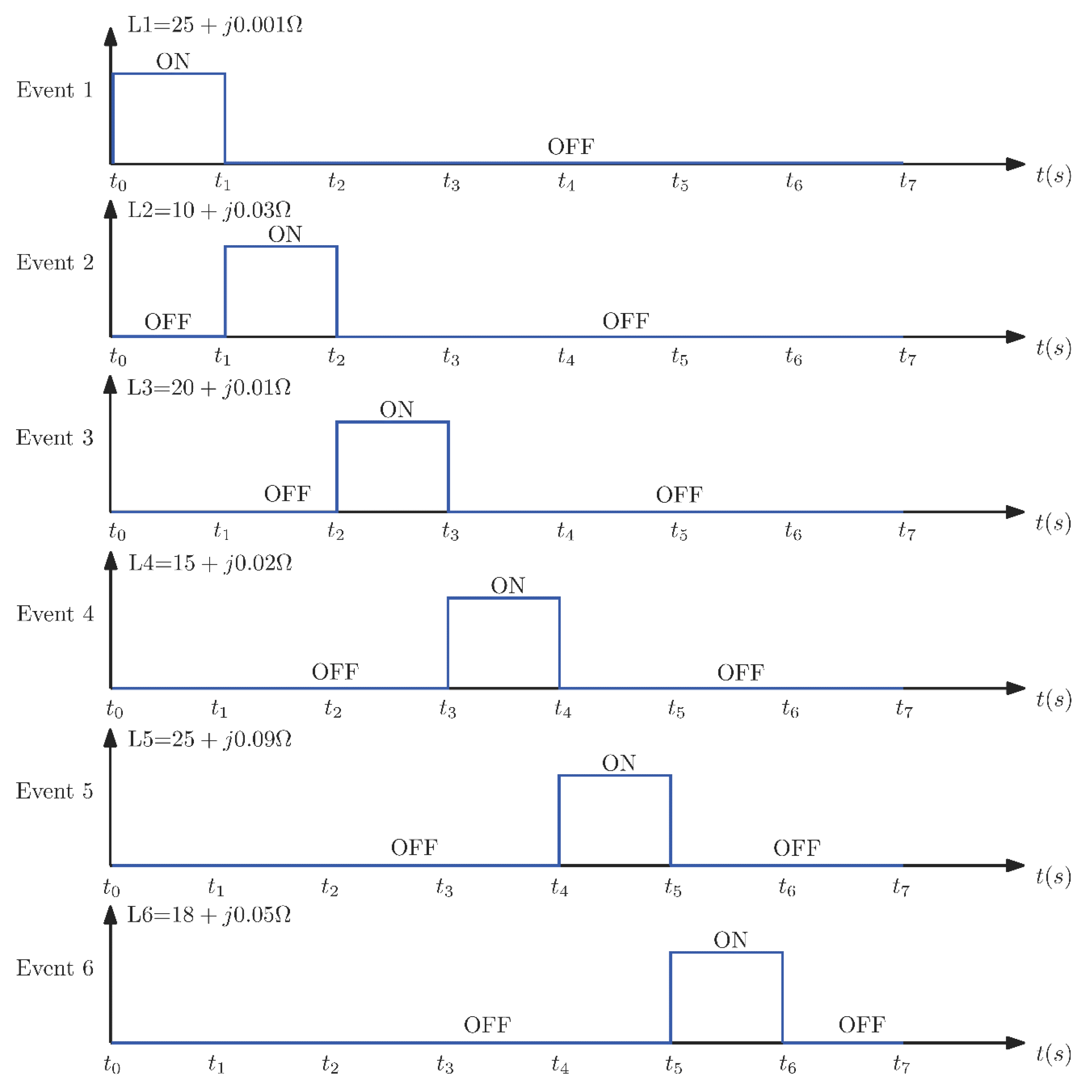
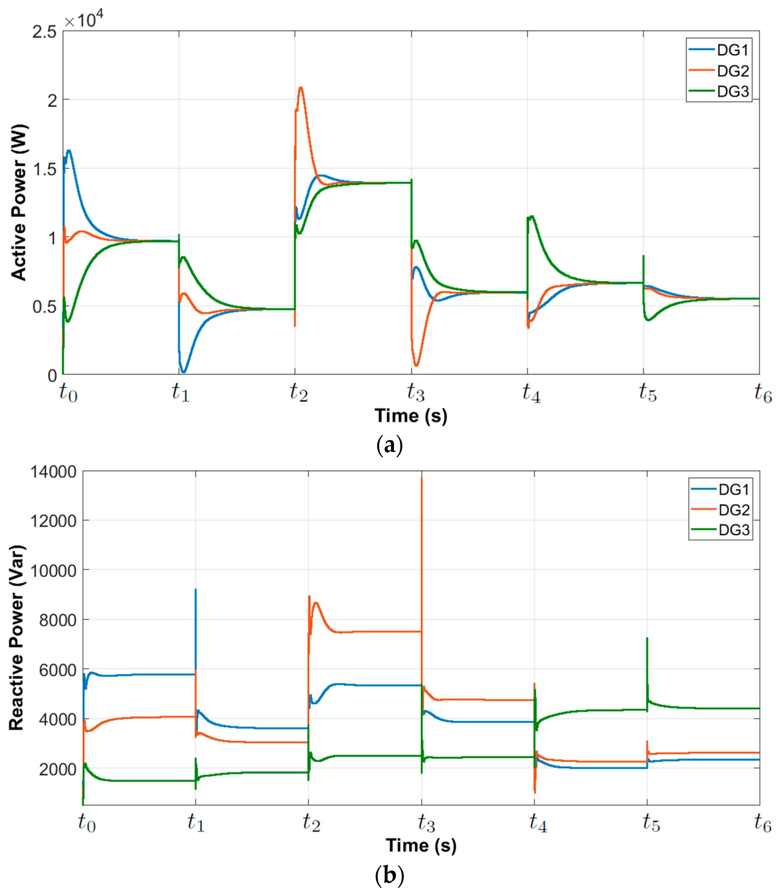
4.3. Multiple Electric Vehicle Connection and Disconnection

In this second test, various EVs are connected and disconnected at different periods and nodes of the microgrid to simulate the increase and decrease of active and reactive power of loads defined in Figure 3 (L1–L6). Figure 10 shows the events at different periods to identify the controller response under multiple EVs connections and disconnections. The following are the six events considered in the connection and disconnection test of multiple EVs.

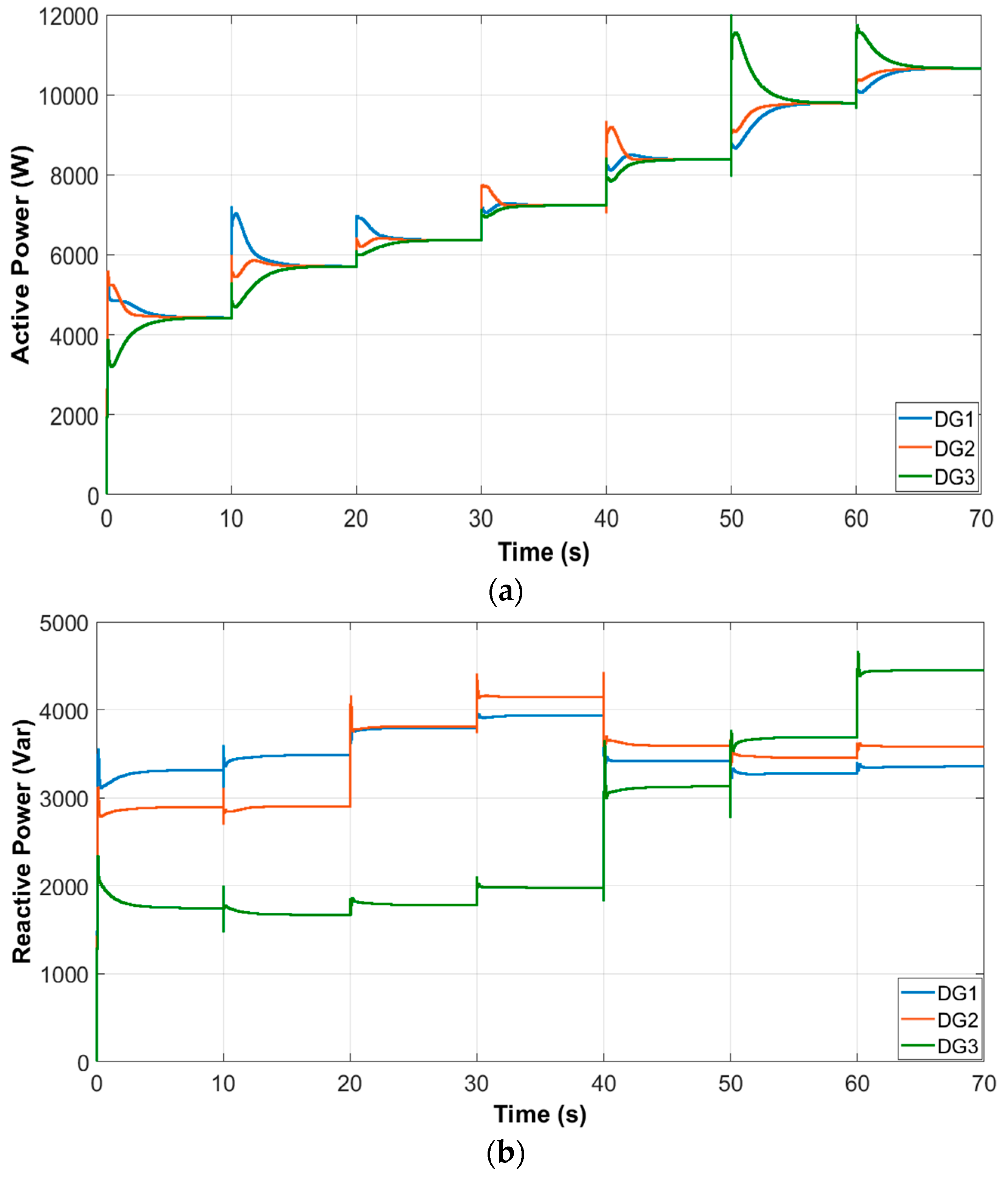
• Event 1: at the beginning of the first period (from $t_0$ to $t_1$), L1 increases the active power consumption after connecting five EVs to Node 1, changing the power by nine times the fixed load of 25 + j0.001 Ω; at the end of the period, this load is disconnected.
• Event 2: at the beginning of the second period (from $t_1$ to $t_2$), the active power increases in L2 when one EV is connected to Node 2, and the power increases by four times its normal value of 10 + j0.03 Ω; at the end of the period, this load is disconnected.
• Event 3: at the beginning of the third period (from $t_2$ to $t_3$), the greatest change of active power is presented in Node 3 (L3) with the connection of 10 EVs, and the consumption in that node is almost 13 times the fixed load of 20 + j0.01 Ω; at the end of the period, this load is disconnected.
• Event 4: at the beginning of the fourth period (from $t_3$ to $t_4$), three EVs are connected to Node 4 (L4), which provides a power consumption of almost five times the average consumption of 15 + j0.02 Ω; at the end of the period, this load is disconnected.
• Event 5: at the beginning of the fifth period (from $t_4$ to $t_5$), the connection of two EVs is presented at Node 5 (L5), resulting in an increase in the load of 22 times the normal active power consumption with respect to the fixed load of 25 + j0.09 Ω; at the end of the period, this load is disconnected.
• Event 6: at the beginning of the sixth period (from $t_5$ to $t_6$), two EVs are connected to Node 6 (L6), which generates an additional power consumption at the node of almost eight times the normal consumption of 18 + j0.05 Ω; at the end of the period, this load is disconnected.

4.3.1. Active and Reactive Power

Figure 11a,b respectively show the active and reactive power supplied to the load when multiple EVs are connected and disconnected in the microgrid. Both active and reactive power increase based on the number of EVs connected to the nodes. It is also observed that powers increase based on the number of EVs connected to the microgrid; i.e., the higher the amount of the vehicles, the more significant the increase of that active and reactive power. In both cases, the control strategy based on variable virtual impedance helps regulate and maintain stability in the power supplied to the load.

4.3.2. Voltage Variations

Figure 12 shows the voltages in different nodes of the network when the EVs are connected and disconnected in the network with the defined events (Events 1–6). It is observed that the voltages tend to reduce slightly when the EVs are connected and increase when they are disconnected. However, in the instant that the EVs are connected to the node, the voltage drops, and immediately the control strategy recovers the magnitude close to the original value. Therefore, the result shows how the control strategy regulates well the signals at different load nodes by using the variable virtual impedance of the network.

4.3.3. Generation Behavior

Figure 13 shows the behavior of the active power in the three DGs when EVs are connected and disconnected. Figure 13a shows the active power, and Figure 13b presents the reactive power. In the simulation, the active power changes each period, corresponding to the connection and disconnection of EVs along the microgrid according to the events previously defined (Events 1–6).

Regarding the active power presented in Figure 13a, the obtained result shows that each distributed generator is stabilized as quickly as possible to deliver adequate active power to the different loads. Thus, the following results are obtained:

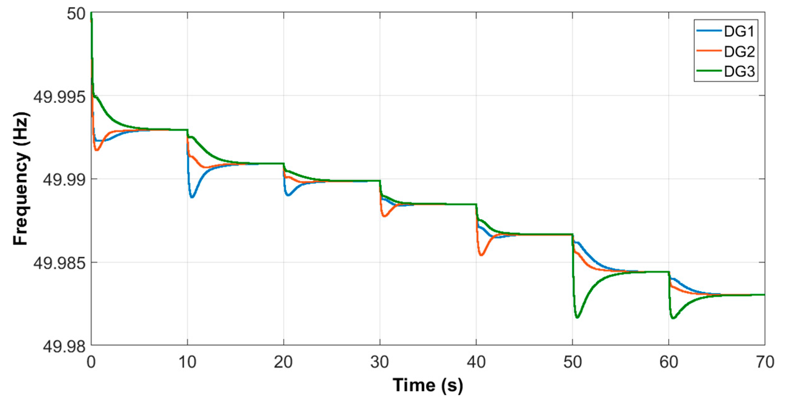
• During the first two periods of simulation (Event 1 and Event 2), the microgrid is subjected to the connection and disconnection of five EVs in Node 1 and followed by one EV connected to Node 2. During these two periods, DGs 1 and 3 are the ones that present the most changes in active power and after some seconds, they finish sharing similar values.
• Then, in the third period (Event 3), 10 EVs are connected to Node 3 at the beginning of the period and disconnected at the end of the period. During this period, DG 2 responds more abruptly to the load change, because this generator is closer than the others to the variable load.
• Later, in the fourth period (Event 4), three EVs are connected to Node 4. In this case, DGs 2 and 3 are the ones that respond most to this load change because they are closest to the load, while the control stabilizes the three generators at the same value of active output power.
• In the fifth period (Event 5), two EVs are connected to Node 5. When analyzing the simulation, the DG that responds more to this change is the DG 3, because it is closest to the variations. However, with the help of the control strategy, the output power is stabilized to the same value as the other two DGs.
• Finally, in the sixth period (Event 6), two EVs are connected to Node 6. In this case, DG 3 undergoes the most abrupt change in power generation, because it is the closest generator to the load.

Regarding the reactive power presented in Figure 13b, the obtained result shows that each distributed generator is stabilized as quickly as possible to deliver adequate reactive power to the different loads. The following results are obtained:

• DG 1 undergoes the most abrupt change in reactive power during the first period (Event 1), because the connection of EVs is closest to this generator.
• Next, during the second period (Event 2), the same generator undergoes the greatest change in reactive power; however, this time with a negative change because it delivers less reactive power because the load decreases 80% at Node 1 (disconnection of five EVs) and Node 2 increases only to one connected EV.
• In the third period (Event 3), DG 3 increases the reactive power because of the load changes from one EV to 10 EVs. Then, the load increases 90%, and DG 2 delivers more reactive power because the EVs are connected to the same node as the generator. Thus, the proposed control strategy performs regulation according to the closest generator.
• In the fourth period (Event 4), the power reduces in DGs 1 and 2 because of the load change from 10 EVs at Node 3 to only three EVs connected at Node 4.
• In the fifth period (Event 5), the powers of DGs 1 and 2 are reduced because three EVs are disconnected from Node 4 and two EVs are connected to Node 5. If the connection of EVs occurs at a greater distance from these two DGs and much closer to DG 3, then the reactive power in DG 3 increases considerably.
• Finally, in the sixth period (Event 6), it is possible to see a slight increase in reactive power delivered by DGs 1, 2, and 3. Although the connection of two EVs at Node 6 is equal to those disconnected from Node 5, the power requirement changes, and they are separated by a line impedance R = 0.321 Ω and L = 6.23 mH; hence, the reactive power delivered from the DGs in the microgrid is increased.

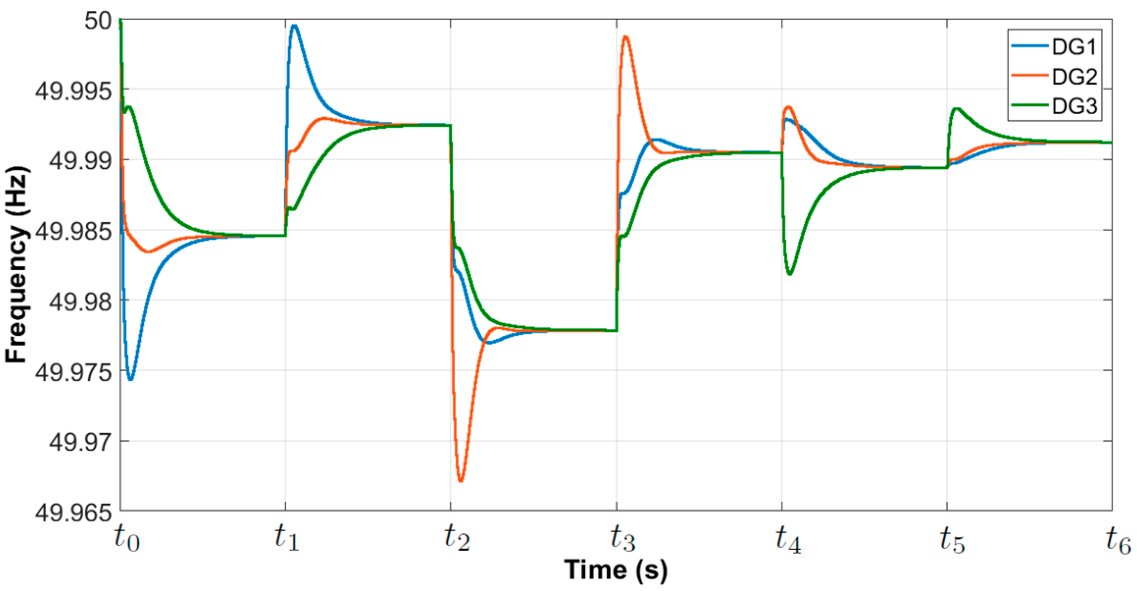
4.3.4. Frequency Regulation

Figure 14 shows the behavior of the output frequency in the three DGs and their variation with load changes. This figure is obtained by considering multiple variations in the power loads as previously described. The results show that the frequency of the three generators stabilizes in a single value a few seconds after the load changes. The larger the change of load in the EV connection, the more abrupt the change in frequency. However, no matter how high the change in the variable load (connection and disconnection of different EVs), the controller maintains the frequency close to 50 Hz, which is the desired value.

5. Conclusions

This paper presented a new control strategy to regulate voltage and share reactive power from distributed generators in a microgrid when EVs are connected and disconnected at different nodes and times. The control strategy considered using fixed and variable virtual impedances created in the microgrid (MG) when loads change or when an EV is connected or disconnected. Results were obtained for a system with three generators, which with the control strategy distribute active power regardless of where the vehicles are connected in the microgrid. It was possible to deliver reactive power according to the place where the load variation is presented. Thus, for a few moments, the reactive power supplied by the distributed generators is increased and, in another period, it is decreased to regulate the voltage in the microgrid. Therefore, this control strategy, based on variable virtual impedance related to the connection distance of EVs, works properly to control the voltage in the different nodes of the microgrid. The control strategy manages to effectively regulate the frequency close to 50 Hz, and the active and reactive power are also maintained to balance the network. This strategy is useful for the new microgrid to adapt and share active and reactive power regardless of the distance where EVs are connected. As only unidirectional vehicles were considered in this research, in future work, bidirectional vehicles should be tested to provide a power backup to the node where the EV is connected.

References

- Neves, S.A.; Marques, A.C.; Fuinhas, J.A. Is energy consumption in the transport sector hampering both economic growth and the reduction of CO2 emissions? A disaggregated energy consumption analysis. Transp. Policy 2017, 59, 64–70. [Google Scholar] [CrossRef]
- Lirola, J.M.; Castã Neda, E.; Lauret, B.; Khayet, M. A review on experimental research using scale models for buildings: Application and methodologies. Energy Build. 2017, 142, 72–110. [Google Scholar] [CrossRef]
- Katiraei, F.; Iravani, M.R. Power Management Strategies for a Microgrid With Multiple Distributed Generation Units. IEEE Trans. Power Syst. 2006, 21, 1821–1831. [Google Scholar] [CrossRef]
- Lasseter, R.H. MicroGrids. In Proceedings of the 2002 IEEE Power Engineering Society Winter Meeting. Conference Proceedings (Cat. No.02CH37309), New York, NY, USA, 27–31 January 2002; Volume 1, pp. 305–308. [Google Scholar]
- Pogaku, N.; Prodanovic, M.; Green, T.C. Modeling, Analysis and Testing of Autonomous Operation of an Inverter-Based Microgrid. IEEE Trans. Power Electron. 2007, 22, 613–625. [Google Scholar] [CrossRef]
- Shaukat, N.; Khan, B.; Ali, S.M.; Mehmood, C.A.; Khan, J.; Farid, U.; Majid, M.; Anwar, S.M.; Jawad, M.; Ullah, Z. A survey on electric vehicle transportation within smart grid system. Renew. Sustain. Energy Rev. 2018, 81, 1329–1349. [Google Scholar] [CrossRef]
- Liu, C.; Chau, K.T.; Wu, D.; Gao, S. Opportunities and Challenges of Vehicle-to-Home, Vehicle-to-Vehicle, and Vehicle-to-Grid Technologies. Proc. IEEE 2013, 101, 2409–2427. [Google Scholar] [CrossRef]
- Pode, R. Battery charging stations for home lighting in Mekong region countries. Renew. Sustain. Energy Rev. 2015, 44, 543–560. [Google Scholar] [CrossRef]
- Diyun, W.; Chau, K.T.; Gao, S. Multilayer framework for vehicle-to-grid operation. In Proceedings of the 2010 IEEE Vehicle Power and Propulsion Conference, Lille, France, 1–3 September 2010; pp. 1–6. [Google Scholar]
- Yilmaz, M.; Krein, P.T. Review of the Impact of Vehicle-to-Grid Technologies on Distribution Systems and Utility Interfaces. IEEE Trans. Power Electron. 2013, 28, 5673–5689. [Google Scholar] [CrossRef]
- Romo, R.; Micheloud, O. Power quality of actual grids with plug-in electric vehicles in presence of renewables and micro-grids. Renew. Sustain. Energy Rev. 2015, 46, 189–200. [Google Scholar] [CrossRef]
- Guille, C.; Gross, G. A conceptual framework for the vehicle-to-grid (V2G) implementation. Energy Policy 2009, 37, 4379–4390. [Google Scholar] [CrossRef]
- Frieske, B.; Kloetzke, M.; Mauser, F. Trends in vehicle concept and key technology development for hybrid and battery electric vehicles. In Proceedings of the 2013 World Electric Vehicle Symposium and Exhibition (EVS27), Barcelona, Spain, 17–20 November 2013; pp. 1–12. [Google Scholar]
- Sovacool, B.K.; Kester, J.; Noel, L.; de Rubens, G.Z. Contested visions and sociotechnical expectations of electric mobility and vehicle-to-grid innovation in five Nordic countries. Environ. Innov. Soc. Transit. 2019, 31, 170–183. [Google Scholar] [CrossRef]
- Ilo, A. “Link”—The smart grid paradigm for a secure decentralized operation architecture. Electr. Power Syst. Res. 2016, 131, 116–125. [Google Scholar] [CrossRef]
- Green, J.; Newman, P. Citizen utilities: The emerging power paradigm. Energy Policy 2017, 105, 283–293. [Google Scholar] [CrossRef]
- Matko, V.; Brezovec, B. Improved Data Center Energy Efficiency and Availability with Multilayer Node Event Processing. Energies 2018, 11, 2478. [Google Scholar] [CrossRef]
- De Ridder, F.; D’Hulst, R.; Knapen, L.; Janssens, D. Applying an Activity based Model to Explore the Potential of Electrical Vehicles in the Smart Grid. Procedia Comput. Sci. 2013, 19, 847–853. [Google Scholar] [CrossRef]
- Lei, S.; Xu, H.; Li, D.; Zhang, Z.; Han, Y. The photovoltaic charging station for electric vehicle to grid application in Smart Grids. In Proceedings of the 2012 IEEE 6th International Conference on Information and Automation for Sustainability, Beijing, China, 27–29 September 2012; pp. 279–284. [Google Scholar]
- Aliasghari, P.; Mohammadi-Ivatloo, B.; Alipour, M.; Abapour, M.; Zare, K. Optimal scheduling of plug-in electric vehicles and renewable micro-grid in energy and reserve markets considering demand response program. J. Clean. Prod. 2018, 186, 293–303. [Google Scholar] [CrossRef]
- Tan, K.M.; Ramachandaramurthy, V.K.; Yong, J.Y. Integration of electric vehicles in smart grid: A review on vehicle to grid technologies and optimization techniques. Renew. Sustain. Energy Rev. 2016, 53, 720–732. [Google Scholar] [CrossRef]
- Stanev, R. A control strategy and operation paradigm for electrical power systems with electric vehicles and distributed energy ressources. In Proceedings of the 2016 19th International Symposium on Electrical Apparatus and Technologies (SIELA), Bourgas, Bulgaria, 29 May–1 June 2016; pp. 1–4. [Google Scholar]
- Hapsari, A.P.N.; Kato, T.; Takahashi, H.; Sasai, K.; Kitagata, G.; Kinoshita, T. Multiagent-based microgrid with electric vehicle allocation planning. In Proceedings of the 2013 IEEE 2nd Global Conference on Consumer Electronics—GCCE 2013, Tokyo, Japan, 1–4 October 2013; pp. 436–437. [Google Scholar]
- Haes Alhelou, H.S.; Golshan, M.E.H.; Fini, M.H. Multi agent electric vehicle control based primary frequency support for future smart micro-grid. In Proceedings of the 2015 Smart Grid Conference (SGC), Tehran, Iran, 22–23 December 2015; pp. 22–27. [Google Scholar]
- Yang, Z.; Duan, B.; Chen, M.; Zhu, Z. A proactive operation strategy of electric vehicle charging-discharging in Photovoltaic micro-grid. In Proceedings of the 2016 IEEE Power & Energy Society Innovative Smart Grid Technologies Conference (ISGT), Minneapolis, MN, USA, 6–9 September 2016; pp. 1–5. [Google Scholar]
- De Brabandere, K.; Bolsens, B.; Van den Keybus, J.; Woyte, A.; Driesen, J.; Belmans, R. A Voltage and Frequency Droop Control Method for Parallel Inverters. IEEE Trans. Power Electron. 2007, 22, 1107–1115. [Google Scholar] [CrossRef]
- Coelho, E.A.A.; Cortizo, P.C.; Garcia, P.F.D. Small signal stability for single phase inverter connected to stiff AC system. In Proceedings of the Conference Record of the 1999 IEEE Industry Applications Conference, Phoenix, AZ, USA, 3–7 October 1999; pp. 2180–2187. [Google Scholar] [CrossRef]
© 2019 by the authors. Licensee MDPI, Basel, Switzerland. This article is an open access article distributed under the terms and conditions of the Creative Commons Attribution (CC BY) license (http://creativecommons.org/licenses/by/4.0/).
Share and Cite
Molina, E.; Candelo-Becerra, J.E.; Hoyos, F.E. Control Strategy to Regulate Voltage and Share Reactive Power Using Variable Virtual Impedance for a Microgrid. Appl. Sci. 2019, 9, 4876. https://doi.org/10.3390/app9224876
Molina E, Candelo-Becerra JE, Hoyos FE. Control Strategy to Regulate Voltage and Share Reactive Power Using Variable Virtual Impedance for a Microgrid. Applied Sciences. 2019; 9(22):4876. https://doi.org/10.3390/app9224876
Chicago/Turabian StyleMolina, Eder, John E. Candelo-Becerra, and Fredy E. Hoyos. 2019. "Control Strategy to Regulate Voltage and Share Reactive Power Using Variable Virtual Impedance for a Microgrid" Applied Sciences 9, no. 22: 4876. https://doi.org/10.3390/app9224876
APA StyleMolina, E., Candelo-Becerra, J. E., & Hoyos, F. E. (2019). Control Strategy to Regulate Voltage and Share Reactive Power Using Variable Virtual Impedance for a Microgrid. Applied Sciences, 9(22), 4876. https://doi.org/10.3390/app9224876