Article

Optimization Based on Product and Desirability Functions for Flow Distribution in Multi-Channel Cooling Systems of Power Inverters in Electric Vehicles

AI & Mechanical Center, Institute for Advanced Engineering, Youngin-si 17180, Korea
*
Author to whom correspondence should be addressed.
Appl. Sci. 2019, 9(22), 4844; https://doi.org/10.3390/app9224844
Submission received: 7 October 2019 / Revised: 6 November 2019 / Accepted: 7 November 2019 / Published: 12 November 2019
(This article belongs to the Section Mechanical Engineering)

Abstract

:
The onboard charger (OBC)/low-voltage DC-DC converter (LDC) integrated power inverter for electric vehicles comprises multiple electrical elements that can heat up, which can cause performance degradation and system instability issues in electric vehicles. To address this, a cooling system is included in the OBC/LDC integrated power inverter, which primarily uses water as a coolant. In this water cooling method, controlling the flow rate of water is critical for uniform cooling of the component. Thus, we propose an optimization method that helps determine the design variables to ensure uniform flow rate in each channel of the water-cooled system. The control variables for fluid-flux flow distribution optimization are selected by performing flow analysis for the initial design shape and analyzing their effects on fluid-flux flow distribution. For optimization analysis, the central composite design technique was applied; in addition, multi-response surface optimization using the same flow rate for each channel was performed. The optimization results were compared and verified using desirability functions based on the flow ratio of the cooling water channel, product function, and error function. Among single-response objective functions, the product function showed excellent performance. However, optimization using a multi-response objective function showed significantly higher prediction accuracy than the single-response function: using the optimized design obtained with the multi-response objective function improved the fluid-flux flow distribution uniformity by approximately 90% or more than the initial design.

1. Introduction

In recent times, owing to the proliferation of electric vehicles (EVs), there has been increased interest in enhancing the energy density of EV power storage as well as improving the efficiency of its components; one such approach involves integrating power inverters with low-voltage DC-DC converters (LDCs) and on-board chargers (OBCs), all of which are key components in EVs. In particular, an OBC is a device that charges a vehicle battery by converting AC power from external sources to DC power, while an LDC converts high-voltage vehicle battery power to low-voltage power that is suitable for operating audio and other electronic systems onboard the vehicle [1]. One approach to achieve high performance and reduce the weight of an EV is developing an EV model that includes devices that perform multiple functions simultaneously by integrating core components into one device [2]. In this light, for LDCs, research on hybrid bidirectional LDC design technology based on high-efficiency two-stage design technology and parallel control techniques for power inverters has been conducted [3,4]. Furthermore, for integrating an LDC and OBC, miniaturization is critical for both circuit package design as well as cooling optimization to realize lightweight EVs. To this end, several efforts have been made in previous studies [4,5,6]. In general, there are two cooling methods for power inverters, namely air cooling and water cooling; however, water cooling is preferred. The most important design consideration to maximize the cooling efficiency in EVs is the appropriate arrangement of flow channels to obtain a uniform flow rate. In addition, this optimization design should be convenient and cost-effective [7]. Therefore, analytical methods have been used in several studies on channel networks to efficiently optimize flow rate distribution. Brkić and Praks proposed the hardy cross method for calculating channel network flow distribution [8,9]. Also, Kim, Yoo, and Cho analyzed incompressible looped flow networks using constitutive topologic matrix equations [10]. Furthermore, water distribution networks were analyzed by Niazkar and Afzali using MATLAB and Excel spreadsheets [11,12]. Moosavian and Jaefarzadeh performed hydraulic analysis of the water supply networks using a modified hardy cross method [13], while Singh, Kheer, and Pandita analyzed water distribution networks based on topological similarity [14]. Moreover, the finite element method (FEM) and finite difference method (FDM) are often used to analyze complex structures such as the channel networks in EV cooling systems [15,16,17]. Though there are many different optimization methods, the one wherein experimental and computational fluid dynamics (CFD) analyses are combined, is used widely; in addition, various algorithms are being studied [18,19,20,21]. However, these studies see that the method of evaluating the system and setting the multi-objective function is insufficient. In particular, Jeong proposed an optimization method wherein the objective function was based on weighted mean and distribution [22]. Furthermore, optimization methods based on the multi-dimensional desirability function are also used in various fields [23,24]. These methods lack the degree of convergence of optimization and the diversity of multi-objective functions as described above. In summary, it is very important to derive the objective function that is suitable for the environment and that represents the system performance function, and various studies on them are necessary. In other words, optimizing multiple general-purpose functions using only response functions cannot guarantee high accuracy of prediction. In addition, in order to increase the accuracy of prediction for multiple responses of the system, a study on the process of deriving the ability to quantitatively evaluate the performance of a system is required.
Therefore, in this study, we propose a method to normalize the response to the target distribution and use it as a multi-objective function of optimization. In addition, we present a method to quantify by product and error distance functions as a system evaluation performance, and propose a method to increase the accuracy of optimization by extending this to the multiple objective function of the system response. Furthermore, this theoretical method is applied to the optimal design method for controlling the distribution of cooling water in the multi-channel flow path of a power inverter system integrated with LDC and OBC, and we present the optimization and verification process. The optimization has been conducted to the distribution control of the cooling water in the flow of the multi-channel network of a power inverter system integrated with LDC and OBC. To evaluate the system performance, product and error distance functions are introduced as optimization objective functions, in which the optimal conditions for distributed uniform flow inside flow channels for our designed cooling plate are obtained. Moreover, the response prediction equation is derived based on the central composite design technique using the response surface methodology. Our optimization results are compared using CFD analysis and various response functions. Then, the optimal design variables for the system are determined by analyzing the pressure difference between the fluid flow behavior and channel based on the above mentioned CFD analysis. Finally, the obtained results are applied to the initial design model to obtain an improved model with a uniform flow rate.

2. Numerical Model and Analysis

2.1. Analysis Model and Governing Equations

The OBC/LDC-integrated power inverter charge/discharge module has a complex structure that includes various electronic components and circuits. The power inverter used in this study is composed of a top cover, main body, cooling plate, and bottom cover. The top and bottom covers are sealed together to protect the electronic components and circuit boards placed inside the module. The main body supports and protects the inner circuits and components. Further, the cooling plate, which is present in the middle, consists of top and bottom plates, and includes the flow multi-channel for cooling water that cools the heated electrical elements in the inverter; these top and bottom plates prevent the leakage of cooling water from the cooling plate. CFD analysis is used to examine the flow characteristics of this cooling water; however, for ease of analysis, the complex real model needs to be simplified based on the purpose of analysis. In particular, for this study, the analytical model can be simplified considering only the cooling water flow path, which is sufficient to examine flow behavior. The basic structure of the OBC/LDC-integrated power inverter used in this study is shown in Figure 1, and the specifications are shown in Table 1.
The governing equations for flow analysis that are used to verify the flow characteristics of the cooling system include the following steady-state equations [16,17]:
· ( ρ u ) = 0
· ( ρ u u ) = P +   · ( u   u )
· ( ρ k u ) = [ ( μ + μ t σ k ) k ] + G k + G b ρ ε Y M
· ( ρ ε u ) = · [ ( μ + μ t σ k ) ε ] + C 1 ε ε k ( G k + C 3 ε G b ) C 2 ε ρ ε 2 k

2.2. CFD Analysis of Concept Model and Corresponding Results

The initial channel design for the cooling system consists of six channels with geometrically identical areas assuming that the incoming cooling water is uniformly distributed among the channels. For uniform cooling efficiency, it is important that the flow rate of cooling water is the same in each flow channel. We examine the flow characteristics of the cooling water by performing CFD analysis based on this initial design model. The density and dynamic viscosity of the water used for cooling is 1000 kg/m3 and 0.001 N-s/m3. The allowable inflow volume of cooling water of OBC is designed to be about 9 L/min. Checking the convergence of the results of the pretest analysis, the element size was determined to be 0.7 mm, and the number of elements is about 1.95 × 10⁶, and the skewness of mesh quality is 0.78. Figure 2 shows the finite element model and boundary condition of the initial design model.
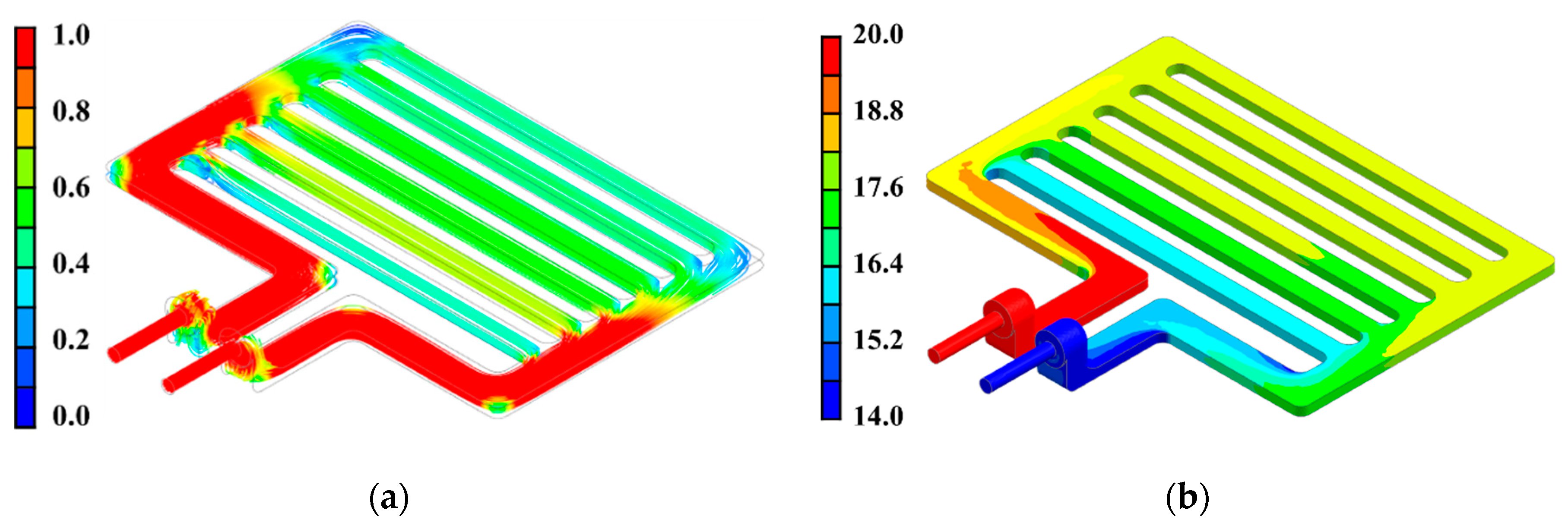
Flow analysis was performed using the ANSYS Fluent 8.0 software. Figure 3 shows the flow analysis results for the flow velocity and pressure as representative flow characteristics. Furthermore, Table 2 lists the average flow velocity and pressure in the different channels as well as the flow volume distribution of the cooling water for each channel along with the normalized values. If the inlet flow volume were the same in each channel, then it would be one-sixth (16.67%) of the total flow. However, as indicated by the values in Table 2, the volume flow ratio of the first cooling water channel is the lowest at 13.19%, while that of the second cooling water channel is the highest at 22.22%. Thus, the maximum-minimum difference of the volume flow rates is as high as 54%; this large deviation in flow volume distribution can be attributed to a directional change in water flow at the first inlet on the cooling plane, which affects the fluid flow due to the momentum generated from the inertia of the fluid. Moreover, as the inflow volume varies by channel, a different dynamic pressure would be realized in each channel. Based on these analysis results and characteristics of Bernoulli’s theorem considering the dynamic flow pressure difference in the different channels, we propose a design improvement that involves changing the shape of the channels to reduce the rotational momentum at the first inlet. Accordingly, we selected inlet volume flow rate and length of the first channel (to control the movement characteristics of the curved part) as design variables to control the flow volume distribution; in addition, we include a rear pipeline based on the dynamic pressure inside the flow channel for pressure balance. Figure 4 highlights the selected design variables that are considered in the improved cooling channel design.

3. Optimal OBC Cooling Plate Design and Results

There are several different optimization methods available in the literature; however, it is important to select a suitable objective function to solve the optimization problem [24]. In this study, product and error distance functions were introduced to improve optimization accuracy, and hence, overall system efficiency. When a random function P ( R i ) can be expressed as a product of the individual responses R i , and it is assumed that the sum of the individual constraint conditions ( Q t ) is constant, then, the product function can be defined as follows [25,26,27]:
Objective function:
P ( R i ) =   i = 1 n R i
Constraint condition:
( R i ) =   i = 1 n R i Q t = 0
If the Lagrange multiplier is used to determine the conditions for the maximum/minimum values of P ( R i ) , we obtain the following function:
L ( R i ,   λ ) =   i = 1 n R i λ (   i = 1 n R i Q t )
Thus, the maximum/minimum value of Equation (7) can be obtained by setting its first-order differentiation to zero:
L ( R , λ ) R i = 0
On solving the first-order differential equation in Equation (8), we obtain the following condition:
R 1 = R 1 · · ·   =   R n
Thus, it is clear that Equation (9) yields the target value of each response R i .
In addition, when   R i , i.e., the flow rate of each channel, is normalized to 1, we get R i =   R i _ r e s p o n s e R i _ t a r g e t ; and assuming that the same flow rate flows in each flow path R i =   n   · R i Q t ; then, the optimization solution can be obtained as P ( R i ) = 1   i = 1 n R i   = 0 . Thus, the following equation can be introduced as the objective function based on the product function:
E ( R i ) d i s t = ( i = 1 n ( 1   n R i Q t ) 2 ) 1 / 2    
Furthermore, using the error of the response value compared with the reference value, another objective function can be set based on the error distance as follows [27,28]:
E ( R i ) m o d = ( 1   i = 1 n n R i Q t ) 2    
The constraint condition for the objective functions in Equations (10) and (11) is the constant total flow rate, which can be expressed as follows:
g ( R i ) =   i = 1 n R i Q t = 0
Thus, Equations (10) and (11) are functions that represent the characteristics of the cooling system. Furthermore, a multi-response objective function can be constructed by combining Equations (10) and (11) along with each response. The optimization algorithm for the multi-response object function can be defined by applying the response surface methodology using the desirability function, i.e., for the multi-response objective function, based on the direct response ( R i ) in Equations (10) and (11), optimization can be achieved using the following desirability objective function [23,26]:
m i n i m i z e [ D ]  
where,
Y =   { 0 y L o w e r   b o u n d T a r g e t L o w e r   b o u n d 1                           i f   Y < L o w e r   b o u n d i f   L o w e r   b o u n d < Y < T a r g e t Y > T a r g e t Y = [ R 1 ,   R 2 ,   , R n , E d i s t ,   E m o d ] D =   ( i = 1 n + 2 Y i q i ) 1 / H ,   H = i = 1 n + 2 q i

3.1. Experimental Design and Numerical Analysis

The design variables for our experiments on numerical optimization were determined based on the central composite design technique, which can be used to effectively construct even second-order functions; in addition, the optimization algorithm was designed using the response surface methodology [20,29]. Without considering the pressure drop, the uniform flow in each channel being the objective of optimization, various objective functions that satisfy the condition of constant total flow rate were established. Considering the design variables described in Section 2, the inlet volume flow rate was set as A, ratio of the length of the gap between the channel and wall and that of the first channel and wall was set as B, and ratio of the width of the rear pipeline to that of the channel was as C. Figure 4 shows the design variables on a schematic figure of the cooling plate, while Table 3 lists the ranges for these design variables. For our numerical analysis, the analysis trial run plan obtained based on the central composite experimental design technique were used, which are listed in Appendix A. The analytical model was constructed in accordance with the experiment sequence, and CFD analysis was performed using the commercial software ANSYS Fluent 8.0. Based on the simulation results, the response values of the response ( R i ) and system characteristic equations, i.e., Equations (10) and (11), were calculated; these are listed in Table 4.
Comparing each case based on the standard deviation of the response value and error function value as listed in Table 4, Case 11 was found to be the worst case, while Case 15 was the optimal case. Figure 5 shows a comparison of the flow velocity and pressure characteristics between the optimal and worst cases. Cases 11 and 15 show clear differences in pressure and velocity; this verifies that the variations of the selected variables influence the responses. Furthermore, in the case of the initial design model (Table 2), the product function value was calculated as 0.313 and the error distance function value as 0.466.

3.2. Optimization and Numerical Validation

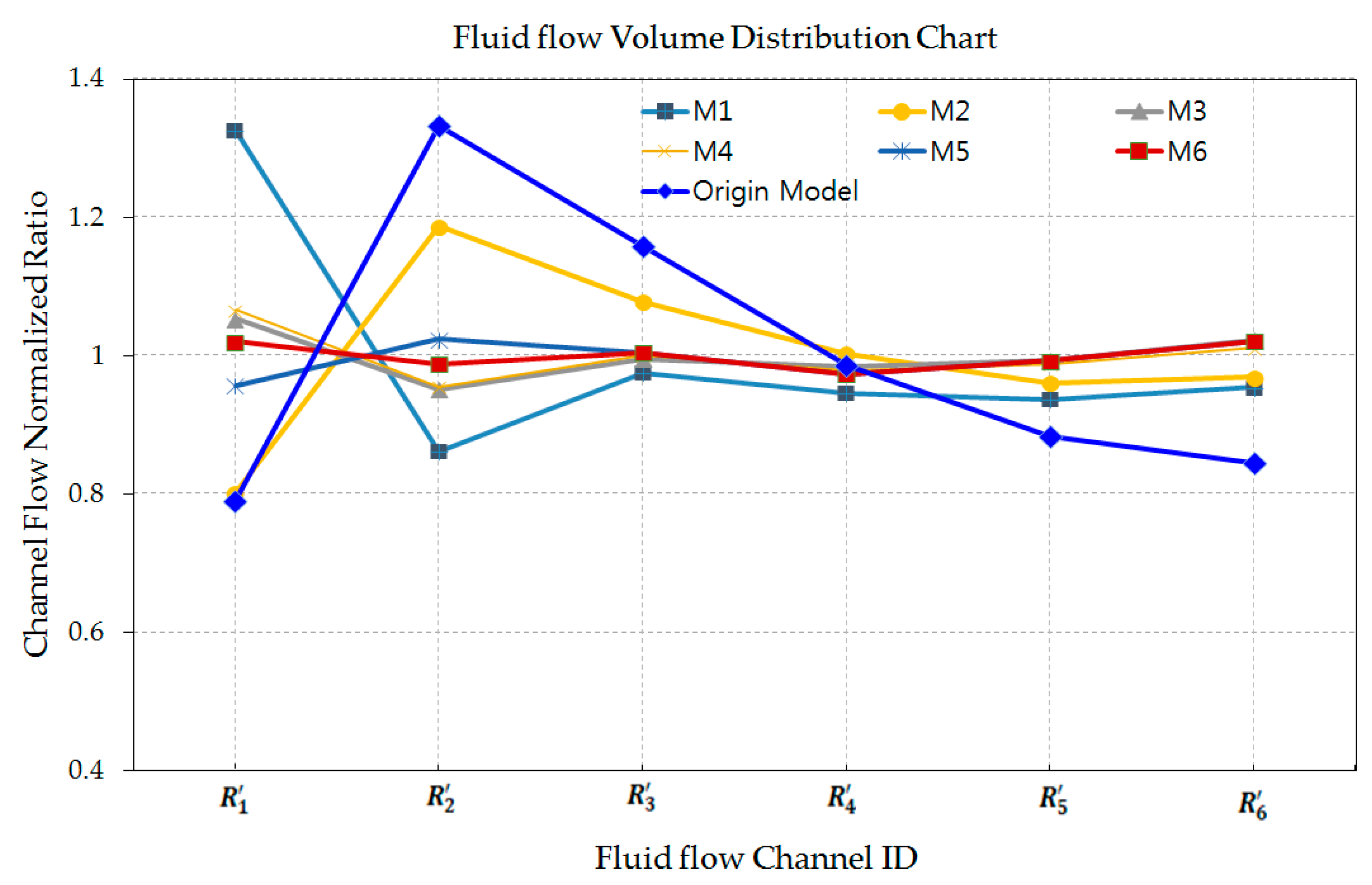
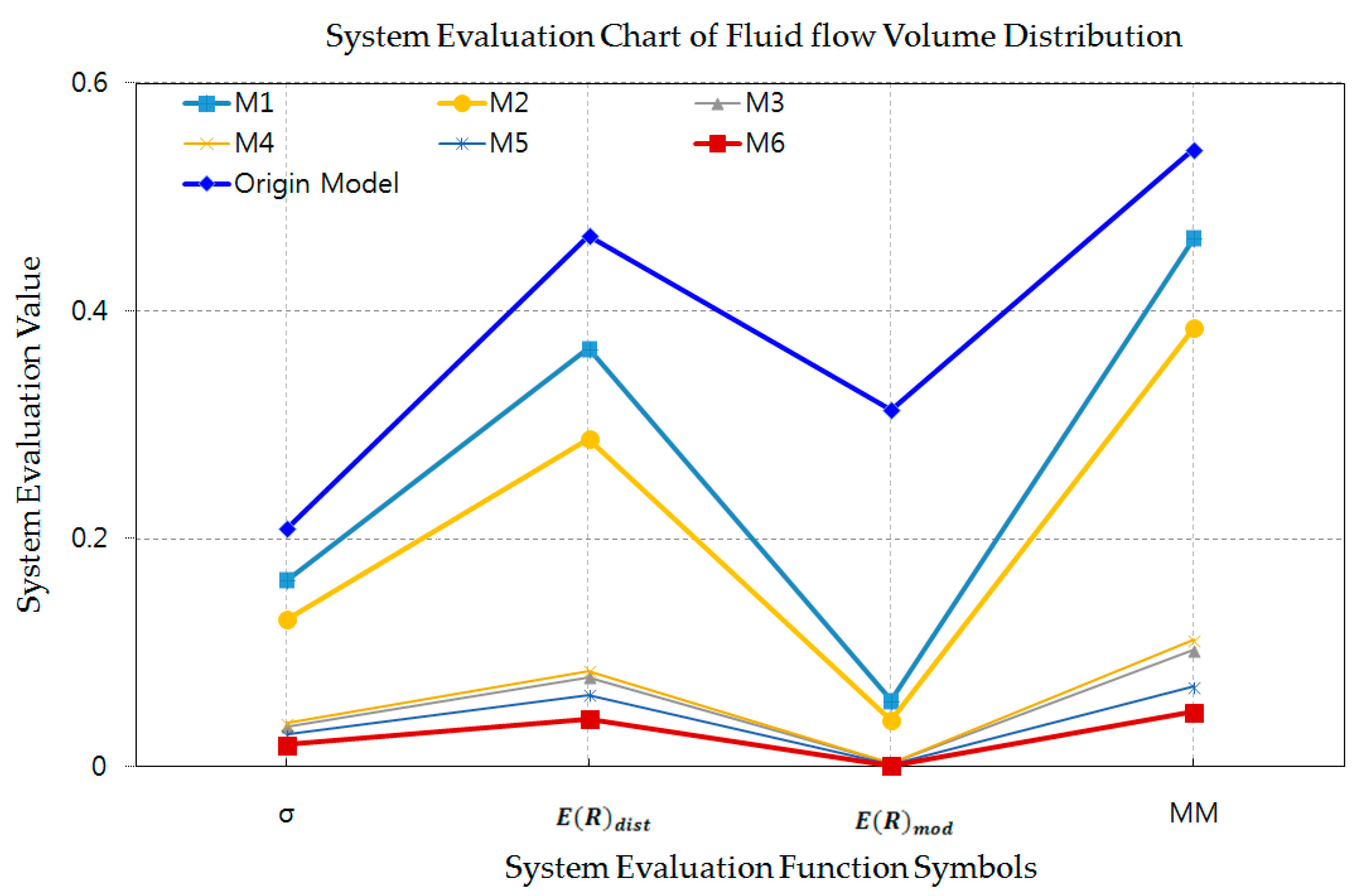
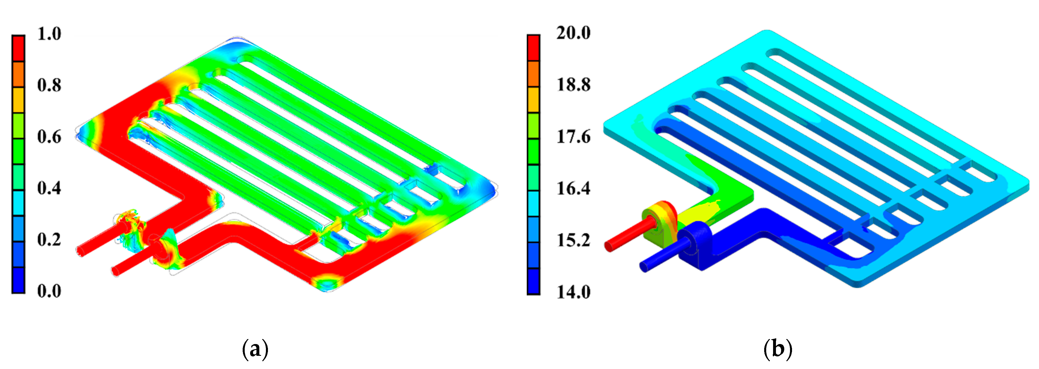
To establish the objective functions for optimization, the expected correlation equations of the response values and variables were derived using the regression analysis method; these functions have been listed in Table 5. For our regression analysis, the stepwise regression analysis method was used [30]. We performed ANOVA analysis of valid variables for stepwise regression analysis of the six response functions in Table 5 as well as the previously introduced system evaluation functions and the results are listed in Appendix A. Based on our results, it can be deduced that variable B is effective in the regression equation of every response function with a p-value of lower than 0.01 for every response except for R 3 and E ( R ) d i s t ; this suggests that design variable B is the most influential factor among the system characteristics, followed by C, and then the interaction between B and C. In contrast, variable A has the lowest influence in determining the flow. Furthermore, based on the regression model, multiple correlation coefficients (R2) for the mean variation measurement values, except for R 3 , have values higher than 0.8. Six different cases for optimization were constructed by combining different product and error distance functions for the volume flow ratio and response value of each channel described in Section 3.1. First, optimization was performed based on the single-response objective function using the product function or error distance function to represent the system. In addition, the response surface optimization methodology was used for constructing a multi-response objective function by combining the volume flow ratio response prediction function, product function, and error distance function for each channel. Table 6 lists the design variable values as well as the composite desirability values obtained via this optimization. In each case, the composite desirability value after optimization was higher than approximately 0.94, which is close to the maximum value of 1; in particular, it was highest when the product function was used for optimization. Next, in the verification stage, the variables (A, B, C) obtained for each optimization case were applied to the design model; this modified model was then verified through simulation. These simulation results are listed in Table 7 and as shown Figure 6 and Figure 7. Furthermore, the velocity and pressure optimization analysis results obtained using the multi-response object function composed of all functions for Case M6 are shown in Figure 8. On comparing the initial model in Figure 3 with the optimized M6 model in Figure 6, it is clear that the velocity distribution difference related to flow rate significantly improved. The optimization results were evaluated based on the standard deviation of the responses for each channel ( R 1   ~ R 6 ), difference between maximum and minimum values, product function values, and error distance function values.
Based on the values listed in Table 7 and as shown Figure 7 and Figure 8, the different cases can be arranged in descending order of prediction accuracy for the optimal variables: M1 < M2 < M4 < M3 < M5 < M6. Thus, for the single-response optimization, optimization using the product function ( E ( R ) m o d ) proposed in this study showed a higher uniformity than using the error distance function ( E ( R ) d i s t ). Furthermore, prediction that is more accurate is possible via optimization based on the multi-response object function than using the single-response object function. In particular, in the case of the multi-response surface optimization design, the prediction accuracy of the design variables can be improved by additionally introducing the system response functions E ( R ) d i s t and E ( R ) m o d in the multi-response object function proposed in this study, rather than using the multi-response object function composed only of direct response functions.
As previously mentioned, the maximum-minimum difference in the volume flow ratio (Table 2) for the initial model is 0.54 with a standard deviation is 0.21; in contrast, in the case of the optimized model (Table 5), the maximum-minimum difference is 0.464 for M1, and 0.048 for M6, with the reduced standard deviations of 0.164 and 0.019, respectively. These results suggest that the optimal design with the most suitable design conditions can be obtained using the proposed objective function (Equation (13)).

4. Conclusions

The flow characteristics of the cooling system used in OBC/LDC integrated power inverters were analyzed through flow analysis of different design models. In addition, based on these characteristics, an optimization method was applied to achieve the same flow rate through each channel in the cooling system. Then, the obtained optimized model was verified via a flow uniformity evaluation method. In summary, the following conclusions can be drawn from this study:
  • For the improved prediction accuracy of the optimized approximation values, the product and error distance functions, and normalized functions of the target value to the response were proposed as the optimization functions to ensure target distribution control in each multi-response.
  • The effective variables for controlling the distribution of flow rate in each channel of a planar cooling structure include the cooling water inlet volume flow rate, ratio of the width of the rear pipeline to that of the channel, and ratio of the length of the gap between the channel and wall to that of first channel and wall. Among these, the most effective variable was found to be the ratio of the length of the gap between the channel and wall to that of the first channel and wall.
  • The product and error distance functions and normalized response functions were applied as the optimization functions to ensure uniform distribution of water in each cooling water channel; it was found that this improved the prediction accuracy of the optimized approximation values.
  • The results of surface response optimization using the desirability function with the central composite design approach for our experimental evaluation indicated that the accuracy of optimization could be more significantly improved using a multi-response object function compared with using single-response object functions.
  • The proposed method was applied to the cooling system of the OBC/LDC integrated power inverter and was found to be highly effective in controlling uniform flow distribution in each cooling water channel. In particular, the flow uniformity among the different channels using the optimized design was more than or equal to 90% than the initial design model in terms of standard deviation, error distance, and maximum-minimum difference.
This study was carried out using an analytical method in a design stage, and will be verified later by an experimental method.

Author Contributions

D.-J.H. designed the equations of motion, conducted numerical programing and simulation, analyzed the results, composed and organized the data, and wrote the paper; S.-H.J. contributed to the numerical analysis and experiment design and data analysis; S.-I.S. contributed to the design and C.A.D; J.-H.N. contributed to the CFD numerical analysis. All authors read and approved the final manuscript.

Funding

This research was funded by the Korea Evaluation Institute of Industrial Technology (KEIT), Ministry of Trade, Industry & Energy (MOTIE), and Daewoo Electronic Components Co. Ltd. via Grant Number No. 10077362.

Conflicts of Interest

The authors declare no conflict of interest.

Nomenclature

A inlet volume flow rate
B length ratio of the gap between the channel and the wall to the first channel
C width ratio of the rear pipeline to the channel
D desirability function
P pressure, Pa
T temperature, K
D O F degree of freedom
R i response for channel i
E ( R ) d i s t error distance function
E ( R ) m o d product function
Q t total flow rate
u fluid velocity m/s
C 1 ε constant
C 2 ε constant
C 3 ε constant
G b production of turbulence kinetic energy due to buoyancy, kg/s3-m
G k production of turbulence kinetic energy due to the mean velocity gradient, kg/s3-m
V i n l e t velocity of inlet, m/s
nnumber of responses
ttime, s
σ standard deviation
α confidence value
ε dissipation rate of turbulent kinetic energy, m2/s3
μ viscosity, Pa-s
ρ density, kg/m3
μ t turbulent viscosity, Pa-s
σ k turbulent Prandtl number for k
σ ε turbulent Prandtl number for ε
q i importance for response i

Appendix A

Table A1. Running case plan for design constraints based on the response surface central composite experimental design technique.
Trial Run No.ABC
Dimension-LessUnit (mm)Dimension-LessUnit (mm)Dimension-LessUnit (mm)
11.0006.0001.00017.1500.4004.000
22.00012.0001.00017.1500.4004.000
31.0006.0003.00051.4500.4004.000
42.00012.0003.00051.4500.4004.000
51.0006.0001.00017.1501.20012.000
62.00012.0001.00017.1501.20012.000
71.0006.0003.00051.4501.20012.000
82.00012.0003.00051.4501.20012.000
90.6593.9502.00034.3000.8008.000
102.34114.0502.00034.3000.8008.000
111.5009.0000.3185.4600.8008.000
121.5009.0003.68263.1400.8008.000
131.5009.0002.00034.3000.1271.270
141.5009.0002.00034.3001.47314.730
151.5009.0002.00034.3000.8008.000
Table A2. ANOVA results for the quadratic model ( R 1 ,   R 2 ,   R 3 ,   R 4 ,   R 5 ,   R 6 ,   E ( R ) d i s t E ( R ) m o d ) .
ResponseVariableDOFSum of SquaresMean Square ValuesF-Valuep-Value
R 1 B14.6974.69788.3600.000
C10.2580.2584.8600.042
Residuals170.9040.053
R 2 0.850
R 2 A10.0420.0425.0100.041
B10.2700.27031.9900.000
C10.2390.23928.3800.000
B × B10.1760.17620.8900.000
Residuals150.12650.008
R 2 0.850
R 3 B10.0060.0060.3000.592
B × B10.1970.1979.7400.006
Residuals170.3440.020
R 2 0.370
R 4 B10.1370.13796.2400.000
C10.0480.04834.0400.000
B × B10.0150.01510.7000.005
Residuals160.0230.001
R 2 0.90
R 5 A10.0180.01850.2200.000
B10.3710.3711011.9500.000
C10.1580.158430.3400.000
B × B10.1510.1519411.1400.000
C × C10.0030.0038.7000.011
B × C10.0030.0039.0700.010
Residuals130.0050.000
R 2 0.990
R 6 A10.0390.03935.2400.000
B10.5580.558499.6700.000
C10.2230.223199.3400.000
B × B10.2640.265236.0900.000
C × C10.0130.01311.2300.005
B × C10.0050.0054.4900.054
Residuals130.0150.001
R 2 0.990
E ( R ) d i s t B10.1190.1192.7500.119
C10.0960.0962.2200.159
B × B14.1284.12895.4100.000
C × C10.1680.1683.8800.069
B × C10.4490.44910.3800.006
Residuals140.6060.043
R 2 0.890
E ( R ) m o d B10.1690.16913.5700.002
C10.1190.1199.5700.007
B × B10.2980.29823.8900.000
B × C10.1380.13811.0200.005
Residuals150.1870.012
R 2 0.800

References

  1. Kim, T.H.; Song, H.S.; Lee, B.H.; Lee, C.S.; Kwon, C.S.; Jung, D.Y. Development of the Integrated Power Converter for the Environmentally Friendly Vehicle and Validation of the LDC using Battery HILS. Trans. Korean Inst. Electr. Eng. 2014, 63, 1212–1218. [Google Scholar] [CrossRef]
  2. Kim, Y.S.; Oh, C.Y.; Sung, W.Y.; Lee, B.K. Topology and Control Scheme of OBC-LDC Integrated Power Unit for Electric Vehicles. IEEE Trans. Power Electron. 2016, 32, 1731–1743. [Google Scholar] [CrossRef]
  3. Lee, B.K.; Gwak, T.G.; Kim, S.G.; Kim, S.J.; Kim, J.P.; Lee, J.Y. High-efficiency 6.6kW LDC/OBC integration structure for electric vehicles. Korean Inst. Power Electron. 2014, 1, 311–312. [Google Scholar]
  4. Kim, H.B.; Jeong, J.W.; Bae, S.W.; Kim, J.S. Design and Implementation of 1.8kW Bi-directional LDC with Parallel Control Strategy for Mild Hybrid Electric. Korean Inst. Power Electron. 2017, 22, 75–81. [Google Scholar] [CrossRef]
  5. Lee, I.O. Research on the analysis and improvement of the performance of the phase-shifted full-bridge converter for electric vehicle battery charger applications. Trans. Korean Inst. Power Electron. 2015, 20, 479–490. [Google Scholar] [CrossRef]
  6. Kim, Y.S.; Oh, C.Y.; Sung, W.Y.; Lee, B.K.; Park, G.C. Optimal design and control of OBC-LDC integrated power unit for electric vehicles. In Proceedings of the 2014 IEEE Applied Power Electronics Conference and Exposition (APEC 2014), Fort Worth, TX, USA, 16 March 2014; pp. 3192–3198. [Google Scholar]
  7. Ye, B.; Rubel, M.R.H.; Li, H. Design and optimization of cooling plate for battery module of an electric vehicle. Appl. Sci. 2019, 9, 754. [Google Scholar] [CrossRef]
  8. Brkić, D.; Praks, P. Short overview of early developments of the hardy cross type methods for computation of flow distribution in pipe networks. Appl. Sci. 2019, 9, 2019. [Google Scholar] [CrossRef]
  9. Yoo, S.Y.; Kim, B.S. A study on the analysis of incompressible and looped flow network using topology constitutive matrix equation. Korean J. Air-Cond. Refrig. Eng. 2010, 22, 573–578. [Google Scholar]
  10. Kim, B.S.; Yoo, S.Y.; Cho, W.S. Development of analysis program for incompressible looped flow network using constitutive topologic matrix equation. Int. J. Air-Cond. Refrig. 2012, 20, 1–8. [Google Scholar] [CrossRef]
  11. Niazkar, M.; Afzali, S.H. Analysis of water distribution networks using MATLAB and Excel Spreadsheet: H-Based Methods. Comput. Appl. Eng. Educ. 2017, 25, 129–141. [Google Scholar] [CrossRef]
  12. Niazkar, M.; Afzali, S.H. Analysis of water distribution networks using MATLAB and Excel Spreadsheet: Q-Based Methods. Comput. Appl. Eng. Educ. 2017, 25, 277–289. [Google Scholar] [CrossRef]
  13. Moosavian, N.; Jaefarzadeh, M.R. Hydraulic analysis of water supply networks using a modified hardy cross method. Int. J. Eng. Trans. B Appl. 2014, 27, 1331–1338. [Google Scholar] [CrossRef]
  14. Singh, M.; Kheer, S.K.; Pandita, I.K. Improvement of water distribution networks analysis by topological similarity. Alex. Eng. J. 2016, 55, 1375–1383. [Google Scholar] [CrossRef]
  15. Noh, J.H.; Lee, H.K.; Ko, D.S.; Hur, D.J. A study on the cooling performance of power converter for eco-friendly vehicle using numerical analysis. J. Comput. Fluid Eng. 2018, 23, 92–101. [Google Scholar] [CrossRef]
  16. Noh, J.H.; Ko, D.S.; Lee, S.J.; Hur, D.J. Numerical modeling and performance prediction of COS hydrolysis reactor in an integrated gasification fuel cell in terms of thermo-chemical transport phenomena. Appl. Sci. 2018, 8, 1196. [Google Scholar] [CrossRef]
  17. Park, H.; Yoon, W. Computational fluid dynamics (CFD) modelling and application for sterilization of foods: A review. Processes 2018, 6, 62. [Google Scholar] [CrossRef]
  18. Ansoni, J.L.; Seleghim, P., Jr. Optimal industrial reactor design: Development of a multiobjective optimization method based on a posteriori performance parameters calculated from CFD flow solutions. Adv. Eng. Softw. 2016, 91, 23–35. [Google Scholar] [CrossRef]
  19. Li, L.; Cheng, Z.; Lange, C.F. CFD-based optimization of fluid flow product aided by artificial intelligence and design space validation. Math. Probl. Eng. 2018, 1, 1–14. [Google Scholar] [CrossRef]
  20. Safikhani, H.; Abbassi, A.; Khalkhali, A.; Kalteh, M. Modeling and optimization of nanofluid flow in flat tubes using a combination of CFD and response surface methodology. Heat Transf.-Asian Res. 2014, 44, 377–395. [Google Scholar] [CrossRef]
  21. Mäkelä, M. Experimental design and response surface methodology in energy applications: A tutorial review. Energy Convers. Manag. 2017, 151, 630–640. [Google Scholar] [CrossRef]
  22. Jeong, I.J.; Cho, H.W. A weighted mean squared error approach to multiple response surface optimization. J. Korea Acad.-Ind. Coop. Soc. 2013, 14, 625–633. [Google Scholar]
  23. Lorza, R.; Calvo, M.; Labari, C. Using the multi-response method with desirability functions to optimize the zinc electroplating of steel screws. Metals 2018, 8, 711. [Google Scholar] [CrossRef]
  24. Jeong, I.J. A posterior preference articulation method to the weighted error minimization approach in multi-response surface optimization. J. Korea Acad.-Ind. Coop. Soc. 2015, 16, 7061–7070. [Google Scholar]
  25. Mishra, S.K. A brief history of production functions. IUP J. Manag. Econ. 2007, 1, 1–25. [Google Scholar] [CrossRef]
  26. Chevillard, S. The functions erf and erfc computed with arbitrary precision and explicit error bounds. Inf. Comput. 2012, 216, 72–95. [Google Scholar] [CrossRef]
  27. Akçay, H.; Anagün, A.S. Multi response optimization application on a manufacturing factor. Math. Comput. Appl. 2013, 18, 531–538. [Google Scholar]
  28. Seok, W.; Kim, G.H.; Seo, J.; Rhee, S.H. Application of the design of experiments and computational fluid dynamics to bow design improvement. J. Mar. Sci. Eng. 2019, 7, 226. [Google Scholar] [CrossRef]
  29. Marjavaara, D.; Lundström, S. Response surface-based shape optimization of a Francis draft tube. Int. J. Numer. Methods Heat Fluid Flow 2007, 17, 34–45. [Google Scholar] [CrossRef]
  30. Wang, K.; Chen, Z. Stepwise regression and all possible subsets regression in education. Electron. Int. J. Educ. Arts Sci. 2016, 2, 60–81. [Google Scholar]
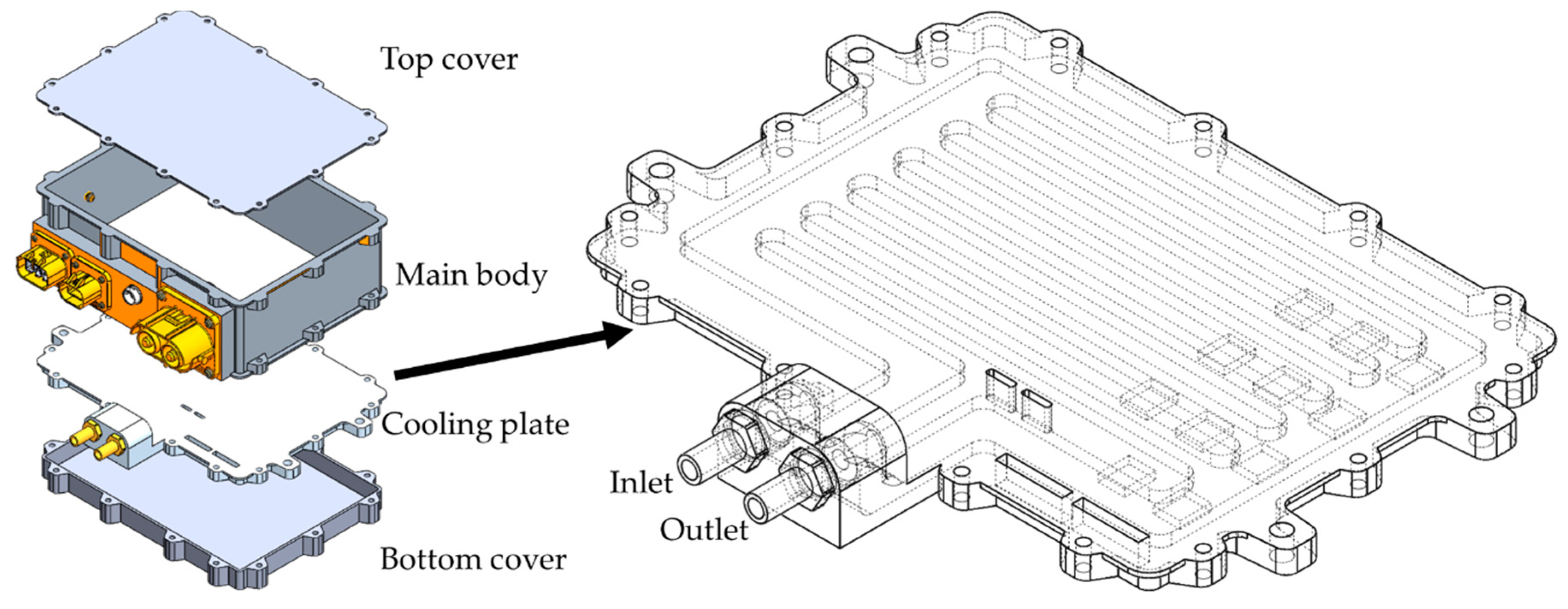
Figure 1. Schematic structure of the OBC/LDC power inverter system with its cooling plate layout.
Applsci 09 04844 g001
Figure 2. Finite element model and boundary condition for computational fluid dynamics (CFD) analysis.
Applsci 09 04844 g002
Figure 3. Velocity and pressure distributions for initial cooling model obtained via CFD: (a) velocity (m/s), (b) pressure (kPa). (The 2 numbers are R1, R2, ..., R6 from the inlet.).
Applsci 09 04844 g003
Figure 4. Design variables for the OBC/LDC flow multi-channel model.
Applsci 09 04844 g004
Figure 5. Comparison of velocity and pressure distributions via flow analysis: (a) velocity [m/s] of the experimental design model in Case 11; (b) pressure [kPa] of the experimental design model in Case 11; (c) velocity [m/s] of the experimental design model in Case 15; (d) pressure [kPa] of the experimental design model in Case 15.
Applsci 09 04844 g005
Figure 6. Comparison of verified response values for the optimal design model based on the obtained analysis results.
Applsci 09 04844 g006
Figure 7. Comparison of system evaluation values for the optimal design model based on the obtained analysis results.
Applsci 09 04844 g007
Figure 8. Velocity and pressure distributions for the optimal M6 model based on CFD analysis: (a) velocity (m/s); (b) pressure (kPa).
Applsci 09 04844 g008
Table 1. Specification of the onboard charger/low-voltage DC-DC converter (OBC/LDC) power inverter system.
FunctionParameterSpecificationUnit
Charging (OBC)Input Voltage85~265V, AC
Input Current32A
Output Current20A, DC
Output Power7.2kW
Power density1.44kW/L
Inverter (Bidirectional)Input Voltage240~450V, DC
Output Voltage85~265V, AC
Output Power3.3kW
Size 250 × 180 × 110mm
Table 2. Characteristic fluid dynamics metrics for initial cooling model obtained via CFD analysis.
ChannelPressure [kPa]Velocity [m/s]Volume Flow [m3/s]Volume Flow Distribution [%]Normalized Volume FlowDistribution N [%]
R116.1980.3960.02013.1870.791
R217.2000.6670.03322.2231.333
R317.6760.5790.02919.3151.159
R417.9320.4930.02516.4420.987
R518.0740.4420.02214.7390.884
R618.1080.4230.02114.0940.846
σ 0.7340.1040.0053.4750.208
MM1.9100.2710.0149.0360.542
MM Ratio [%]10.9554.20054.200--
σ   : Standard Deviation, MM: Max-Min, M M   R a t i o [ % ] = M M A v e r a g e ( R ) .
Table 3. Upper and lower bounds for the values of design variables.
VariablesLimit
DimensionlessSI Units (mm, LPM)
LowerUpperLowerUpper
A1.0002.0006.00012.000
B1.0003.00017.15051.450
C0.4001.2004.00012.000
Table 4. Response values of the response surface experimental design model based on the analysis results.
CaseFluid Flow Volume Distribution [Ratio]SDDistance Error Function ValueProduct Function Value
R 1 R 2 R 3 R 4 R 5 R 6 σ E ( R ) d i s t E ( R ) m o d
10.4941.1391.1001.0771.0831.1070.2490.5560.201
20.3431.0771.0811.1051.1661.2280.3270.7310.368
31.8400.7160.9240.8620.8310.8260.4170.9330.28
41.8290.6190.9040.8750.8770.8950.4200.9400.297
50.0930.8811.0621.2221.3361.4050.4831.0800.800
60.0770.7290.9891.2391.4251.5400.5391.2060.849
71.6690.4990.8880.9490.9871.0080.3780.8450.302
81.6530.3300.8440.9781.0701.1240.4290.9590.458
91.3410.8940.9800.9420.9180.9240.1700.3790.061
101.2140.7280.9340.9891.0371.0980.1640.3680.07
110.6680.5240.2621.1541.5741.8190.6171.3800.697
121.8720.370.8330.9240.9761.0250.4881.0920.467
131.5941.0471.0030.8480.7650.7440.3160.7060.192
141.0790.6330.9371.0521.1251.1730.1960.4390.112
151.2470.7740.9490.9771.0041.0480.1530.3430.058
SD: Standard Deviation.
Table 5. Expected response regression functions based on the response data of the analyzed response surface design.
TypeARegression Equation
Fluid volume ratio of channel0.05 R 1 = 0.265 + 0.5865 B - 0.344 C
R 2 = 1.091 − 0.1113 A + 0.2977 B − 0.3310 C − 0.1096 B xB
R 3 = 0.495 + 0.484 B − 0.1159 B*B
R 4 = 1.1919 − 0.2287 B + 0.1487 C + 0.03217 B*B
R 5 = 1.2713 + 0.0734 A − 0.5312 B + 0.5188 C + 0.10178 B*B − 0.0925 C*C − 0.0510 B*C
R 6 = 1.3471 + 0.1073 A − 0.6903 B + 0.738 C + 0.13456 B*B − 0.1834 C*C − 0.0626 B*C
EFV E ( R ) d i s t = 0.123 − 0.419 B + 0.889 C + 0.1425 B*B − 0.3278 B*C
MFV E ( R ) m o d = 1.775 − 1.750 B + 0.320 C + 0.5325 B*B + 0.672 C*C − 0.592 B*C
EFV: Error Function Value E ( R ) d i s t , MFV: Multiply Function Value E ( R ) m o d , α : Confidence Value.
Table 6. Design variable data obtained via optimization using the expected response regression function.
CaseObject Function TypeObject FunctionTargetABCComposite Desirability
M1Single Function E ( R ) d i s t 0.000-2.0000.64370.9549
M2 E ( R ) m o d 0.000-1.19390.34981.0000
M3Multiple Function R 1 R 6 1.0001.0671.64330.65730.9603
M4 R 1 R 6 , E ( R ) d i s t 1.000, 0.0001.0161.67170.68440.9430
M5 R 1 R 6 , E ( R ) m o d 1.000, 0.0001.4241.45790.44980.9765
M6 R 1 R 6 , E ( R ) d i s t , E ( R ) m o d 1.000, 0.000, 0.0001.4071.56070.52570.9411
Table 7. Verified response values for the optimal design model based on the obtained analysis results.
CaseFluid Flow Volume Distribution [Ratio]SDEFVMFVMax-Min
R 1 R 2 R 3 R 4 R 5 R 6 σ E ( R ) d i s t E ( R ) m o d MM
M11.3260.8620.9750.9460.9370.9540.1640.3670.0580.464
M20.8021.1871.0781.0030.9610.9690.1290.2880.0410.385
M31.0530.9510.9950.9840.9941.0230.0350.0780.0030.102
M41.0660.9551.0010.9790.9881.0110.0380.0840.0030.111
M50.9571.0241.0050.9730.9931.0210.0280.0630.0020.070
M61.0200.9881.0050.9730.9931.0210.0190.0420.0010.048
Origin Model0.7911.3331.1590.9860.8840.8450.2090.4660.3130.542
SD: Standard Deviation, EFV: Error Function Value, MFV: Multiply Function Value.