Solving the Manufacturing Cell Design Problem through an Autonomous Water Cycle Algorithm

 ,
,  ,
,  ,
,  ,
,  ,
, 
Abstract
:1. Introduction
2. Related Work
3. The Manufacturing Cell Design Problem
3.1. Problem Statement
- Modeling parameters:
- -
- M: the number of machines.
- -
- P: the number of parts.
- -
- C: the number of cells.
- -
- : the maximum number of machines in a cell.
- -
- : the element in the machine-part incidence matrix, meaningwhere } is the machine number and is the part number.
- Decision variables:
- -
- : the element in the machine-cell incidence matrix, meaningwhere } is the cell number.
- -
- : the element in the part-cell incidence matrix, meaning
3.2. Problem Example
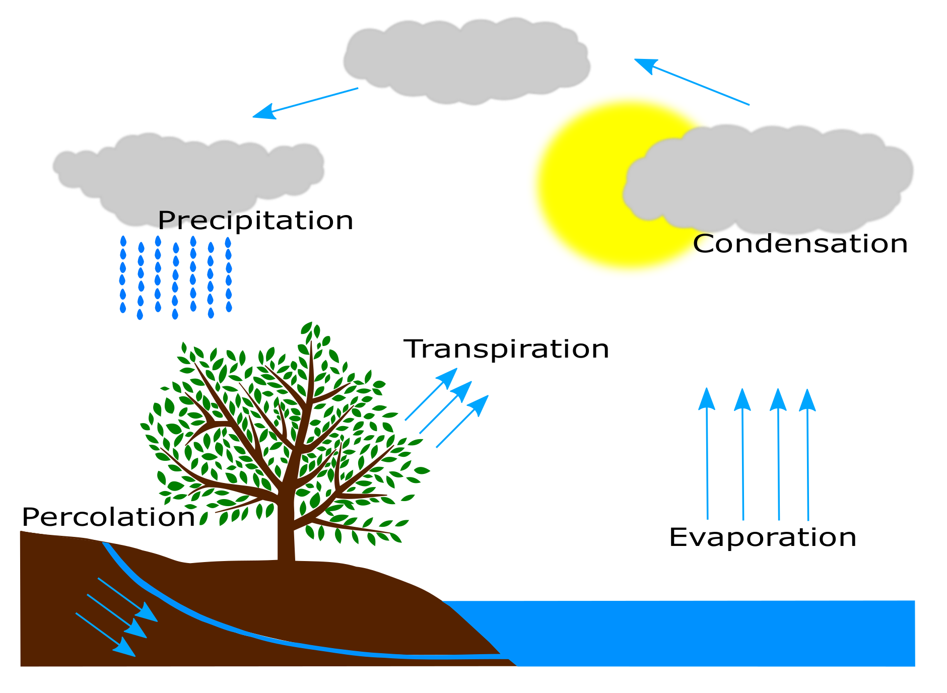
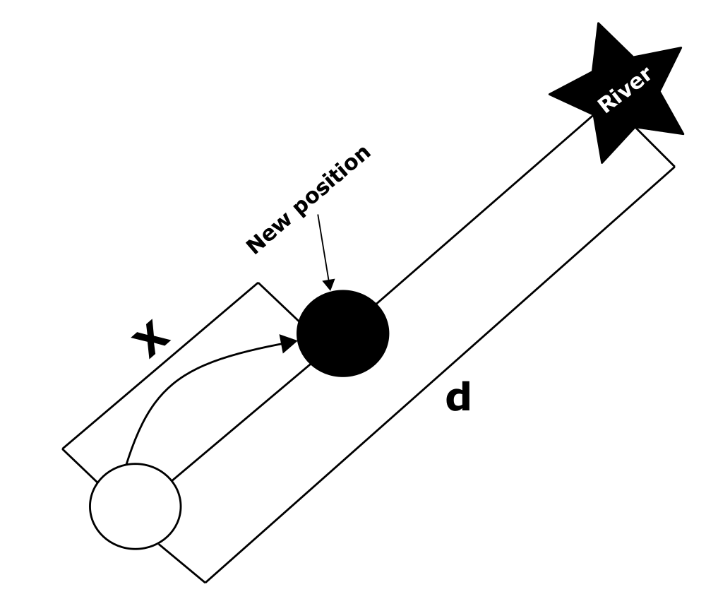
4. The Water Cycle Inspired Solving-Method
| Algorithm 1: Water cycle inspired algorithm. |
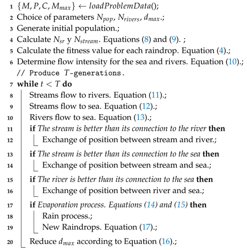 |
5. The Proposed Autonomous Water Cycle Algorithm
| Algorithm 2: Hybridization of autonomous search and the water cycle algorithm. |
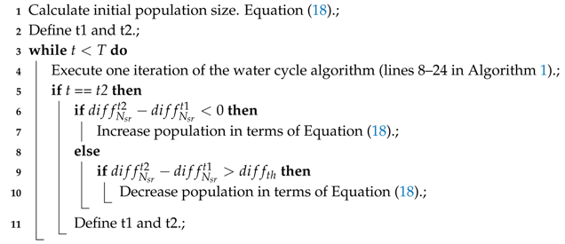 |
6. Experimental Analysis
6.1. Experimental Methodology
6.2. Discussion of the Experimental Results
7. Conclusions
Author Contributions
Funding
Acknowledgments
Conflicts of Interest
References
- Flanders, R.E. Design, manufacture, and production control of a standard machine. Trans. Am. Soc. Mech. Eng. 1924, 46, 691–738. [Google Scholar]
- Soto, R.; Kjellerstrand, H.; Durán, O.; Crawford, B.; Monfroy, E.; Paredes, F. Cell formation in group technology using constraint programming and Boolean satisfiability. Expert Syst. Appl. 2012, 39, 11423–11427. [Google Scholar] [CrossRef]
- Soto, R.; Kjellerstrand, H.; Gutiérrez, J.; López, A.; Crawford, B.; Monfroy, E. Solving Manufacturing Cell Design Problems Using Constraint Programming. In Advanced Research in Applied Artificial Intelligence; Springer: Berlin/Heidelberg, Germany, 2012; pp. 400–406. [Google Scholar]
- Moon, C.; Gen, M. A genetic algorithm-based approach for design of independent manufacturing cells. Int. J. Prod. Econ. 1999, 60–61, 421–426. [Google Scholar] [CrossRef]
- Xambre, A.; Vilarinho, P. A simulated annealing approach for manufacturing cell formation with multiple identical machines. Eur. J. Oper. Res. 2003, 151, 434–446. [Google Scholar] [CrossRef]
- Huang, C.; Li, Y.; Yao, X. A Survey of Automatic Parameter Tuning Methods for Metaheuristics. IEEE Trans. Evol. Comput. 2019. [Google Scholar] [CrossRef]
- Eskandar, H.; Sadollah, A.; Bahreininejad, A.; Hamdi, M. Water cycle algorithm—A novel metaheuristic optimization method for solving constrained engineering optimization problems. Comput. Struct. 2012, 110–111, 151–166. [Google Scholar] [CrossRef]
- Sadollah, A.; Eskandar, H.; Lee, H.M.; Yoo, D.G.; Kim, J.H. Water cycle algorithm: A detailed standard code. SoftwareX 2015, 5, 37–43. [Google Scholar] [CrossRef]
- Hamadi, Y.; Monfroy, E.; Saubion, F. What Is Autonomous Search? In Hybrid Optimization; Springer: New York, NY, USA, 2010; pp. 357–391. [Google Scholar]
- Črepinšek, M.; Liu, S.H.; Mernik, M. Exploration and exploitation in evolutionary algorithms: A survey. ACM Comput. Surv. (CSUR) 2013, 45, 35. [Google Scholar] [CrossRef]
- Boctor, F.F. A Jinear formulation of the machine-part cell formation problem. Int. J. Prod. Res. 1991, 29, 343–356. [Google Scholar] [CrossRef]
- Burbidge, J.L. Production flow analysis for planning group technology. J. Oper. Manag. 1991, 10, 5–27. [Google Scholar] [CrossRef]
- Purcheck, G.F.K. A Linear-Programming Method for the Combinatorial Grouping of an Incomplete Power Set. J. Cybern. 1975, 5, 51–76. [Google Scholar] [CrossRef]
- Oliva-López, E.; Purcheck, G.F. Load balancing for group technology planning and control. Int. J. Mach. Tool Des. Res. 1979, 19, 259–274. [Google Scholar] [CrossRef]
- Kusiak, A.; Chow, W.S. Efficient solving of the group technology problem. J. Manuf. Syst. 1987, 6, 117–124. [Google Scholar] [CrossRef]
- Albadawi, Z.; Bashir, H.A.; Chen, M. A mathematical approach for the formation of manufacturing cells. Comput. Ind. Eng. 2005, 48, 3–21. [Google Scholar] [CrossRef]
- Sankaran, S.; Rodin, E.Y. Multiple objective decision making approach to cell formation: A goal programming model. Math. Comput. Model. 1990, 13, 71–81. [Google Scholar] [CrossRef]
- Shafer, S.M.; Rogers, D.F. A goal programming approach to the cell formation problem. J. Oper. Manag. 1991, 10, 28–43. [Google Scholar] [CrossRef]
- Aljaber, N.; Baek, W.; Chen, C.L. A tabu search approach to the cell formation problem. Comput. Ind. Eng. 1997, 32, 169–185. [Google Scholar] [CrossRef]
- Lozano, S.; Adenso-Diaz, B.; Eguia, I.; Onieva, L. A One-Step Tabu Search Algorithm for Manufacturing Cell Design. J. Oper. Res. Soc. 1999, 50, 509–516. [Google Scholar] [CrossRef]
- Chang, C.C.; Wu, T.H.; Wu, C.W. An efficient approach to determine cell formation, cell layout and intracellular machine sequence in cellular manufacturing systems. Comput. Ind. Eng. 2013, 66, 438–450. [Google Scholar] [CrossRef]
- Lei, D.; Wu, Z. Tabu search-based approach to multi-objective machine-part cell formation. Int. J. Prod. Res. 2005, 43, 5241–5252. [Google Scholar] [CrossRef]
- Chung, S.H.; Wu, T.H.; Chang, C.C. An efficient tabu search algorithm to the cell formation problem with alternative routings and machine reliability considerations. Comput. Ind. Eng. 2011, 60, 7–15. [Google Scholar] [CrossRef]
- Venugopal, V.; Narendran, T. A genetic algorithm approach to the machine-component grouping problem with multiple objectives. Comput. Ind. Eng. 1992, 22, 469–480. [Google Scholar] [CrossRef]
- Gupta, Y.; Gupta, M.; Kumar, A.; Sundaram, C. A genetic algorithm-based approach to cell composition and layout design problems. Int. J. Prod. Res. 1996, 34, 447–482. [Google Scholar] [CrossRef]
- Lee, M.K.; Luong, H.; Abhary, K. A genetic algorithm based cell design considering alternative routing. Comput. Integr. Manuf. Syst. 1997, 10, 93–108. [Google Scholar] [CrossRef]
- Chan, F.T.S.; Lau, K.W.; Chan, L.Y.; Lo, V.H.Y. Cell formation problem with consideration of both intracellular and intercellular movements. Int. J. Prod. Res. 2008, 46, 2589–2620. [Google Scholar] [CrossRef]
- Chiang, C.P.; Lee, S.D. A genetic-based algorithm with the optimal partition approach for the cell formation in bi-directional linear flow layout. Int. J. Comput. Integr. Manuf. 2004, 17, 364–375. [Google Scholar] [CrossRef]
- Imran, M.; Kang, C.; Lee, Y.H.; Jahanzaib, M.; Aziz, H. Cell formation in a cellular manufacturing system using simulation integrated hybrid genetic algorithm. Comput. Ind. Eng. 2017, 105, 123–135. [Google Scholar] [CrossRef]
- Chan, F.T.; Lau, K.; Chan, P.; Choy, K. Two-stage approach for machine-part grouping and cell layout problems. Robot. Comput.-Integr. Manuf. 2006, 22, 217–238. [Google Scholar] [CrossRef]
- Nsakanda, A.L.; Diaby, M.; Price, W.L. Hybrid genetic approach for solving large-scale capacitated cell formation problems with multiple routings. Eur. J. Oper. Res. 2006, 171, 1051–1070. [Google Scholar] [CrossRef]
- Boulif, M.; Atif, K. A new branch-&-bound-enhanced genetic algorithm for the manufacturing cell formation problem. Comput. Oper. Res. 2006, 33, 2219–2245. [Google Scholar]
- Zeb, A.; Khan, M.; Khan, N.; Tariq, A.; Ali, L.; Azam, F.; Jaffery, S.H.I. Hybridization of simulated annealing with genetic algorithm for cell formation problem. Int. J. Adv. Manuf. Technol. 2016, 86, 2243–2254. [Google Scholar] [CrossRef]
- Banerjee, I.; Das, P. Group technology based adaptive cell formation using predator–prey genetic algorithm. Appl. Soft Comput. 2012, 12, 559–572. [Google Scholar] [CrossRef]
- Wu, T.H.; Chang, C.C.; Chung, S.H. A simulated annealing algorithm for manufacturing cell formation problems. Expert Syst. Appl. 2008, 34, 1609–1617. [Google Scholar] [CrossRef]
- Noktehdan, A.; Karimi, B.; Kashan, A.H. A differential evolution algorithm for the manufacturing cell formation problem using group based operators. Expert Syst. Appl. 2010, 37, 4822–4829. [Google Scholar] [CrossRef]
- Tavakkoli-Moghaddam, R.; Javadian, N.; Khorrami, A.; Gholipour-Kanani, Y. Design of a scatter search method for a novel multi-criteria group scheduling problem in a cellular manufacturing system. Expert Syst. Appl. 2010, 37, 2661–2669. [Google Scholar] [CrossRef]
- Durán, O.; Rodriguez, N.; Consalter, L.A. Collaborative particle swarm optimization with a data mining technique for manufacturing cell design. Expert Syst. Appl. 2010, 37, 1563–1567. [Google Scholar] [CrossRef]
- Soto, R.; Crawford, B.; Almonacid, B.; Paredes, F. A Migrating Birds Optimization Algorithm for Machine-Part Cell Formation Problems. In Advances in Artificial Intelligence and Soft Computing, Proceedings of the 14th Mexican International Conference on Artificial Intelligence (MICAI 2015), Cuernavaca, Mexico, 25–31 October 2015; Part I; Springer International Publishing: Cham, Switzerland, 2015; pp. 270–281. [Google Scholar]
- Soto, R.; Crawford, B.; Almonacid, B.; Paredes, F. Efficient Parallel Sorting for Migrating Birds Optimization When Solving Machine-Part Cell Formation Problems. Sci. Program. 2016, 2016, 21. [Google Scholar] [CrossRef]
- Soto, R.; Crawford, B.; Vega, E.; Paredes, F. Solving Manufacturing Cell Design Problems Using an Artificial Fish Swarm Algorithm. In Lecture Notes in Computer Science; Springer International Publishing: Berlin/Heidelberg, Germany, 2015; pp. 282–290. [Google Scholar]
- Soto, R.; Crawford, B.; Vega, E.; Johnson, F.; Paredes, F. Solving Manufacturing Cell Design Problems Using a Shuffled Frog Leaping Algorithm. In Advances in Intelligent Systems and Computing; Springer International Publishing: Berlin/Heidelberg, Germany, 2015; pp. 253–261. [Google Scholar]
- Soto, R.; Crawford, B.; Alarcón, A.; Zec, C.; Vega, E.; Reyes, V.; Araya, I.; Olguín, E. Solving Manufacturing Cell Design Problems by Using a Bat Algorithm Approach. In Lecture Notes in Computer Science; Springer International Publishing: Berlin/Heidelberg, Germany, 2016; pp. 184–191. [Google Scholar]
- Munoz, R.; Olivares, R.; Taramasco, C.; Villarroel, R.; Soto, R.; Alonso-Sánchez, M.F.; Merino, E.; de Albuquerque, V.H.C. A new EEG software that supports emotion recognition by using an autonomous approach. Neural Comput. Appl. 2018. [Google Scholar] [CrossRef]
- Soto, R.; Crawford, B.; Lama, J.; Almonacid, B. A firefly algorithm to solve the manufacturing cell design problem. In Proceedings of the 2016 11th Iberian Conference on Information Systems and Technologies (CISTI), Las Palmas, Spain, 15–18 June 2016; pp. 1–4. [Google Scholar]
- Soto, R.; Crawford, B.; Lama, J.; Paredes, F. A Firefly Algorithm to Solve the Manufacturing Cell Design Problem. In Advances in Intelligent Systems and Computing; Springer International Publishing: Berlin/Heidelberg, Germany, 2016; pp. 103–114. [Google Scholar]
- Soto, R.; Crawford, B.; Toledo, A.A.; de la Fuente-Mella, H.; Castro, C.; Paredes, F.; Olivares, R. Solving the Manufacturing Cell Design Problem through Binary Cat Swarm Optimization with Dynamic Mixture Ratios. Comput. Intell. Neurosci. 2019, 2019. [Google Scholar] [CrossRef]
- Soto, R.; Crawford, B.; Olivares, R.; Conti, M.D.; Rubio, R.; Almonacid, B.; Niklander, S. Resolving the Manufacturing Cell Design Problem Using the Flower Pollination Algorithm. In Lecture Notes in Computer Science; Springer International Publishing: Berlin/Heidelberg, Germany, 2016; pp. 184–195. [Google Scholar]
- Munoz, R.; Olivares, R.; Taramasco, C.; Villarroel, R.; Soto, R.; Barcelos, T.S.; Merino, E.; Alonso-Sánchez, M.F. Using Black Hole Algorithm to Improve EEG-Based Emotion Recognition. Comput. Intell. Neurosci. 2018, 2018. [Google Scholar] [CrossRef]
- Almonacid, B.; Aspée, F.; Soto, R.; Crawford, B.; Lama, J. Solving the manufacturing cell design problem using the modified binary firefly algorithm and the egyptian vulture optimisation algorithm. IET Softw. 2017, 11, 105–115. [Google Scholar] [CrossRef]
- Soto, R.; Crawford, B.; Olivares, R.; Galleguillos, C.; Castro, C.; Johnson, F.; Paredes, F.; Norero, E. Using autonomous search for solving constraint satisfaction problems via new modern approaches. Swarm Evol. Comput. 2016, 30, 64–77. [Google Scholar] [CrossRef]
- Soto, R.; Crawford, B.; Vega, E.; Gómez, A.; Gómez-Pulido, J.A. Solving the Set Covering Problem Using Spotted Hyena Optimizer and Autonomous Search. In Proceedings of the International Conference on Industrial, Engineering and Other Applications of Applied Intelligent Systems, Graz, Austria, 9–11 July 2019; pp. 854–861. [Google Scholar]
- Soto, R.; Crawford, B.; Herrera, R.; Olivares, R.; Johnson, F.; Paredes, F. WSM tuning in autonomous search via gravitational search algorithms. In Artificial Intelligence Perspectives and Applications; Springer: Berlin/Heidelberg, Germany, 2015; pp. 159–168. [Google Scholar]
- Sadollah, A.; Eskandar, H.; Bahreininejad, A.; Kim, J.H. Water cycle algorithm with evaporation rate for solving constrained and unconstrained optimization problems. Appl. Soft Comput. 2015, 30, 58–71. [Google Scholar] [CrossRef]
- Sadollah, A.; Eskandar, H.; Kim, J.H. Water cycle algorithm for solving constrained multi-objective optimization problems. Appl. Soft Comput. 2015, 27, 279–298. [Google Scholar] [CrossRef]
- Heidari, A.A.; Abbaspour, R.A.; Jordehi, A.R. Gaussian bare-bones water cycle algorithm for optimal reactive power dispatch in electrical power systems. Appl. Soft Comput. 2017, 57, 657–671. [Google Scholar] [CrossRef]
- Pahnehkolaei, S.M.A.; Alfi, A.; Sadollah, A.; Kim, J.H. Gradient-based water cycle algorithm with evaporation rate applied to chaos suppression. Appl. Soft Comput. 2017, 53, 420–440. [Google Scholar] [CrossRef]
- Wemmerlöv, U.; Hyer, N.L. Cellular manufacturing in the U.S. industry: A survey of users. Int. J. Prod. Res. 1989, 27, 1511–1530. [Google Scholar] [CrossRef]
- Zhang, Z. Modeling complexity of cellular manufacturing systems. Appl. Math. Model. 2011, 35, 4189–4195. [Google Scholar] [CrossRef]
- Mansouri, S.A.; Husseini, S.M.; Newman, S. A review of the modern approaches to multi-criteria cell design. Int. J. Prod. Res. 2000, 38, 1201–1218. [Google Scholar] [CrossRef]
- Bonoli, A.; Fusco, E.D.; Zanni, S.; Lauriola, I.; Ciriello, V.; Federico, V.D. Green Smart Technology for Water (GST4Water): Life Cycle Analysis of Urban Water Consumption. Water 2019, 11, 389. [Google Scholar] [CrossRef]
- Antunes, L.; Ghisi, E.; Thives, L. Permeable Pavements Life Cycle Assessment: A Literature Review. Water 2018, 10, 1575. [Google Scholar] [CrossRef]
- Hofman-Caris, R.; Bertelkamp, C.; de Waal, L.; van den Brand, T.; Hofman, J.; van der Aa, R.; van der Hoek, J. Rainwater Harvesting for Drinking Water Production: A Sustainable and Cost-Effective Solution in The Netherlands? Water 2019, 11, 511. [Google Scholar] [CrossRef]
- Zahid, A.; Abbas, H.T.; Imran, M.A.; Qaraqe, K.A.; Alomainy, A.; Cumming, D.R.S.; Abbasi, Q.H. Characterization and Water Content Estimation Method of Living Plant Leaves Using Terahertz Waves. Appl. Sci. 2019, 9, 2781. [Google Scholar] [CrossRef]
- Nguyen, H.T.T.; Chao, H.R.; Chen, K.C. Treatment of Organic Matter and Tetracycline in Water by Using Constructed Wetlands and Photocatalysis. Appl. Sci. 2019, 9, 2680. [Google Scholar] [CrossRef]
- Slimani, Z.; Trabelsi, A.; Virgone, J.; Freire, R.Z. Study of the Hygrothermal Behavior of Wood Fiber Insulation Subjected to Non-Isothermal Loading. Appl. Sci. 2019, 9, 2359. [Google Scholar] [CrossRef]
- Calvet, L.; de Armas, J.; Masip, D.; Juan, A.A. Learnheuristics: Hybridizing metaheuristics with machine learning for optimization with dynamic inputs. Open Math. 2017, 15, 261–280. [Google Scholar] [CrossRef]


| Machines | |||||||||||
|---|---|---|---|---|---|---|---|---|---|---|---|
| A | B | C | D | E | F | G | H | I | J | ||
| 1 | ✓ | ✓ | |||||||||
| 2 | ✓ | ✓ | ✓ | ||||||||
| 3 | ✓ | ✓ | ✓ | ✓ | |||||||
| 4 | ✓ | ✓ | |||||||||
| Parts | 5 | ✓ | ✓ | ✓ | |||||||
| 6 | ✓ | ✓ | |||||||||
| 7 | ✓ | ✓ | ✓ | ||||||||
| 8 | ✓ | ✓ | |||||||||
| 9 | ✓ | ✓ | |||||||||
| 10 | ✓ | ✓ | |||||||||
| Cell | Cell | ||||||||
|---|---|---|---|---|---|---|---|---|---|
| 1 | 2 | 3 | 1 | 2 | 3 | ||||
| A | ✓ | 1 | ✓ | ||||||
| B | ✓ | 2 | ✓ | ||||||
| C | ✓ | 3 | ✓ | ||||||
| D | ✓ | 4 | ✓ | ||||||
| Machines | E | ✓ | Parts | 5 | ✓ | ||||
| F | ✓ | 6 | ✓ | ||||||
| G | ✓ | 7 | ✓ | ||||||
| H | ✓ | 8 | ✓ | ||||||
| I | ✓ | 9 | ✓ | ||||||
| J | ✓ | 10 | ✓ | ||||||

| Instance | C | M | Best | Instance | C | M | Best | Instance | C | M | Best |
|---|---|---|---|---|---|---|---|---|---|---|---|
| ID | Known | ID | Known | ID | Known | ||||||
| BP01 | 2 | 8 | 11 | BP11 | 2 | 9 | 11 | BP21 | 2 | 10 | 11 |
| BP02 | 2 | 8 | 7 | BP12 | 2 | 9 | 6 | BP22 | 2 | 10 | 4 |
| BP03 | 2 | 8 | 4 | BP13 | 2 | 9 | 4 | BP23 | 2 | 10 | 4 |
| BP04 | 2 | 8 | 14 | BP14 | 2 | 9 | 13 | BP24 | 2 | 10 | 13 |
| BP05 | 2 | 8 | 9 | BP15 | 2 | 9 | 6 | BP25 | 2 | 10 | 6 |
| BP06 | 2 | 8 | 5 | BP16 | 2 | 9 | 3 | BP26 | 2 | 10 | 3 |
| BP07 | 2 | 8 | 7 | BP17 | 2 | 9 | 4 | BP27 | 2 | 10 | 4 |
| BP08 | 2 | 8 | 13 | BP18 | 2 | 9 | 10 | BP28 | 2 | 10 | 8 |
| BP09 | 2 | 8 | 8 | BP19 | 2 | 9 | 8 | BP29 | 2 | 10 | 8 |
| BP10 | 2 | 8 | 8 | BP20 | 2 | 9 | 5 | BP30 | 2 | 10 | 5 |
| BP31 | 2 | 11 | 11 | BP41 | 2 | 12 | 11 | BP51 | 3 | 6 | 27 |
| BP32 | 2 | 11 | 3 | BP42 | 2 | 12 | 3 | BP52 | 3 | 6 | 7 |
| BP33 | 2 | 11 | 3 | BP43 | 2 | 12 | 1 | BP53 | 3 | 6 | 9 |
| BP34 | 2 | 11 | 13 | BP44 | 2 | 12 | 13 | BP54 | 3 | 6 | 27 |
| BP35 | 2 | 11 | 5 | BP45 | 2 | 12 | 4 | BP55 | 3 | 6 | 11 |
| BP36 | 2 | 11 | 3 | BP46 | 2 | 12 | 2 | BP56 | 3 | 6 | 6 |
| BP37 | 2 | 11 | 4 | BP47 | 2 | 12 | 4 | BP57 | 3 | 6 | 11 |
| BP38 | 2 | 11 | 5 | BP48 | 2 | 12 | 5 | BP58 | 3 | 6 | 14 |
| BP39 | 2 | 11 | 5 | BP49 | 2 | 12 | 5 | BP59 | 3 | 6 | 12 |
| BP40 | 2 | 11 | 5 | BP50 | 2 | 12 | 5 | BP60 | 3 | 6 | 10 |
| BP61 | 3 | 7 | 18 | BP71 | 3 | 8 | 11 | BP81 | 3 | 9 | 11 |
| BP62 | 3 | 7 | 6 | BP72 | 3 | 8 | 6 | BP82 | 3 | 9 | 6 |
| BP63 | 3 | 7 | 4 | BP73 | 3 | 8 | 4 | BP83 | 3 | 9 | 4 |
| BP64 | 3 | 7 | 18 | BP74 | 3 | 8 | 14 | BP84 | 3 | 9 | 13 |
| BP65 | 3 | 7 | 8 | BP75 | 3 | 8 | 8 | BP85 | 3 | 9 | 6 |
| BP66 | 3 | 7 | 4 | BP76 | 3 | 8 | 4 | BP86 | 3 | 9 | 3 |
| BP67 | 3 | 7 | 5 | BP77 | 3 | 8 | 5 | BP87 | 3 | 9 | 4 |
| BP68 | 3 | 7 | 11 | BP78 | 3 | 8 | 11 | BP88 | 3 | 9 | 10 |
| BP69 | 3 | 7 | 12 | BP79 | 3 | 8 | 8 | BP89 | 3 | 9 | 8 |
| BP70 | 3 | 7 | 8 | BP80 | 3 | 8 | 8 | BP90 | 3 | 9 | 5 |
| Instance | M | P | ID | M | C | Best | ID | M | C | Best |
|---|---|---|---|---|---|---|---|---|---|---|
| (Author) | Know | Know | ||||||||
| King | 5 | 7 | CFP01 | 3 | 2 | 0 | CFP02 | 2 | 3 | 2 |
| Waghodekar | 5 | 7 | CFP03 | 3 | 2 | 5 | CFP04 | 2 | 3 | 8 |
| Seifoddini | 5 | 18 | CFP05 | 3 | 2 | 5 | CFP06 | 2 | 3 | 11 |
| Kusiak | 6 | 8 | CFP07 | 3 | 2 | 2 | CFP08 | 2 | 3 | 7 |
| Kusiak | 7 | 11 | CFP09 | 4 | 2 | 3 | CFP10 | 3 | 3 | 5 |
| Boctor | 7 | 11 | CFP11 | 4 | 2 | 2 | CFP12 | 3 | 3 | 2 |
| Seifoddini | 8 | 12 | CFP13 | 4 | 2 | 6 | CFP14 | 3 | 3 | 7 |
| Chandrasekharan | 8 | 20 | CFP15 | 4 | 2 | 7 | CFP16 | 3 | 3 | 14 |
| Chandrasekharan | 8 | 20 | CFP17 | 4 | 2 | 28 | CFP18 | 3 | 3 | 39 |
| Mosier | 10 | 10 | CFP19 | 5 | 2 | 1 | CFP20 | 4 | 3 | 0 |
| Chan | 10 | 15 | CFP21 | 5 | 2 | 4 | CFP22 | 4 | 3 | 0 |
| Askin | 14 | 24 | CFP23 | 7 | 2 | 1 | CFP24 | 5 | 3 | 2 |
| Stanfel | 14 | 24 | CFP25 | 7 | 2 | 2 | CFP26 | 5 | 3 | 22 |
| McCormick | 16 | 24 | CFP27 | 8 | 2 | 16 | CFP28 | 6 | 3 | 17 |
| Srinivasan | 16 | 30 | CFP29 | 8 | 2 | 12 | CFP30 | 6 | 3 | – |
| King | 16 | 43 | CFP31 | 8 | 2 | 15 | CFP32 | 6 | 3 | – |
| Carrie | 18 | 24 | CFP33 | 9 | 2 | 13 | CFP34 | 6 | 3 | – |
| Mosier | 20 | 20 | CFP35 | 10 | 2 | 27 | CFP36 | 7 | 3 | – |
| Kumar | 20 | 23 | CFP37 | 10 | 2 | 25 | CFP38 | 7 | 3 | – |
| Carrie | 20 | 35 | CFP39 | 10 | 2 | 1 | CFP40 | 7 | 3 | – |
| Boe | 20 | 35 | CFP41 | 10 | 2 | – | CFP42 | 7 | 3 | – |
| Chandrasekharan | 24 | 40 | CFP43 | 12 | 2 | – | CFP44 | 8 | 3 | – |
| Chandrasekharan | 24 | 40 | CFP45 | 12 | 2 | – | CFP46 | 8 | 3 | – |
| Chandrasekharan | 24 | 40 | CFP47 | 12 | 2 | – | CFP48 | 8 | 3 | – |
| Chandrasekharan | 24 | 40 | CFP49 | 12 | 2 | – | CFP50 | 8 | 3 | – |
| Chandrasekharan | 24 | 40 | CFP51 | 12 | 2 | – | CFP52 | 8 | 3 | – |
| Chandrasekharan | 24 | 40 | CFP53 | 12 | 2 | – | CFP54 | 8 | 3 | – |
| McCormick | 27 | 27 | CFP55 | 14 | 2 | – | CFP56 | 9 | 3 | – |
| Carrie | 28 | 46 | CFP57 | 14 | 2 | – | CFP58 | 10 | 3 | – |
| Kumar | 30 | 41 | CFP59 | 15 | 2 | – | CFP60 | 10 | 3 | – |
| Stanfel | 30 | 50 | CFP61 | 15 | 2 | – | CFP62 | 10 | 3 | – |
| Stanfel | 30 | 50 | CFP63 | 15 | 2 | – | CFP64 | 10 | 3 | – |
| King | 30 | 90 | CFP65 | 18 | 2 | – | CFP66 | 12 | 3 | – |
| McCormick | 37 | 53 | CFP67 | 19 | 2 | – | CFP68 | 13 | 3 | – |
| Chandrasekharan | 40 | 100 | CFP69 | 20 | 2 | – | CFP70 | 14 | 3 | – |
| Water Cycle Algorithm | |||||||||||||||
|---|---|---|---|---|---|---|---|---|---|---|---|---|---|---|---|
| Instance | Autonomous Approach | Default Approach | |||||||||||||
| ID | |||||||||||||||
| BP01 | 11,631 | 196.71 | 11.13 | 9372 | 157.52 | 11.81 | 11,572 | 115.16 | 11.26 | 13,097 | 169.13 | 11.00 | 13,163 | 149.52 | 11.39 |
| BP02 | 11,427 | 172.71 | 11.00 | 9081 | 137.71 | 11.26 | 11,345 | 80.29 | 11.06 | 12,921 | 71.58 | 11.00 | 13,247 | 46.39 | 11.00 |
| BP03 | 11,572 | 222.68 | 11.00 | 9021 | 178.55 | 11.13 | 10,329 | 126.68 | 11.00 | 12,642 | 72.00 | 11.00 | 13,281 | 90.23 | 11.00 |
| BP04 | 11,594 | 128.81 | 11.16 | 8964 | 156.00 | 11.23 | 11,378 | 158.52 | 11.00 | 12,863 | 118.97 | 11.00 | 12,903 | 61.13 | 11.06 |
| BP05 | 11,311 | 96.58 | 11.15 | 9102 | 146.90 | 11.65 | 10,363 | 211.39 | 11.06 | 12,759 | 154.00 | 11.10 | 13,347 | 136.61 | 11.19 |
| BP06 | 11,601 | 370.87 | 7.03 | 8969 | 135.03 | 7.26 | 11,729 | 241.48 | 7.29 | 12,865 | 264.16 | 7.29 | 12,829 | 252.94 | 7.16 |
| BP07 | 11,872 | 141.26 | 6.15 | 9093 | 111.71 | 6.23 | 11,377 | 96.13 | 6.29 | 13,042 | 82.84 | 6.45 | 13,171 | 65.48 | 6.45 |
| BP08 | 11,646 | 199.06 | 5.10 | 8972 | 136.48 | 5.35 | 11,404 | 178.87 | 4.94 | 12,825 | 144.29 | 4.77 | 13,067 | 142.13 | 4.90 |
| BP09 | 12,054 | 33.35 | 4.26 | 8836 | 86.35 | 4.74 | 11,581 | 74.97 | 3.71 | 12,548 | 35.77 | 4.19 | 13,066 | 70.52 | 4.00 |
| BP10 | 11,942 | 81.61 | 3.37 | 9177 | 106.03 | 3.74 | 11,602 | 47.55 | 3.68 | 12,539 | 114.10 | 3.29 | 13,147 | 72.10 | 3.48 |
| BP11 | 11,723 | 5.97 | 5.38 | 9128 | 8.77 | 4.77 | 11,900 | 3.55 | 5.52 | 12,743 | 1.16 | 5.00 | 13,292 | 0.71 | 5.48 |
| BP12 | 11,606 | 73.65 | 4.39 | 9038 | 52.65 | 4.65 | 11,840 | 40.55 | 4.52 | 12,614 | 46.23 | 4.52 | 13,347 | 55.19 | 4.65 |
| BP13 | 11,576 | 95.94 | 4.13 | 8941 | 178.19 | 4.45 | 11,707 | 114.23 | 4.32 | 12,596 | 65.13 | 4.13 | 13,016 | 69.84 | 4.00 |
| BP14 | 11,384 | 35.26 | 3.15 | 9019 | 37.77 | 3.55 | 10,789 | 16.94 | 3.58 | 12,839 | 26.84 | 3.45 | 13,431 | 11.65 | 3.65 |
| BP15 | 11,365 | 77.19 | 2.15 | 9062 | 36.19 | 2.13 | 11,062 | 31.90 | 2.26 | 12,514 | 7.19 | 2.45 | 13,168 | 49.26 | 2.06 |
| BP16 | 11,449 | 121.23 | 13.15 | 8907 | 199.42 | 14.45 | 11,851 | 251.45 | 14.26 | 12,709 | 203.16 | 14.23 | 13,245 | 226.06 | 14.32 |
| BP17 | 11,478 | 71.32 | 13.00 | 8996 | 53.32 | 13.00 | 10,805 | 48.23 | 13.00 | 12,801 | 23.13 | 13.00 | 13,104 | 20.71 | 13.00 |
| BP18 | 11,272 | 110.13 | 13.00 | 8947 | 68.87 | 13.00 | 10,695 | 96.48 | 13.00 | 12,711 | 63.32 | 13.00 | 13,219 | 58.71 | 13.00 |
| BP19 | 11,334 | 186.81 | 13.19 | 9028 | 127.32 | 13.06 | 11,087 | 140.52 | 13.13 | 12,679 | 169.61 | 13.10 | 13,037 | 85.10 | 13.00 |
| BP20 | 11,416 | 269.32 | 13.10 | 9022 | 167.45 | 13.45 | 11,509 | 192.06 | 13.13 | 12,919 | 186.65 | 13.13 | 13,075 | 142.06 | 13.06 |
| BP21 | 11,444 | 19.61 | 9.14 | 9040 | 3.58 | 9.97 | 11,886 | 0.81 | 9.77 | 12,992 | 4.03 | 9.65 | 12,990 | 1.97 | 9.84 |
| BP22 | 11,413 | 30.97 | 7.03 | 9079 | 52.19 | 7.58 | 11,608 | 23.97 | 7.61 | 12,772 | 9.35 | 7.13 | 13,208 | 11.00 | 7.45 |
| BP23 | 11,118 | 99.03 | 7.02 | 9063 | 65.39 | 7.19 | 10,607 | 23.42 | 7.13 | 12,784 | 85.42 | 7.06 | 12,870 | 119.84 | 7.13 |
| BP24 | 11,397 | 25.55 | 6.27 | 9134 | 99.32 | 7.10 | 11,718 | 76.16 | 6.19 | 12,778 | 61.77 | 5.68 | 13,112 | 59.16 | 6.00 |
| BP25 | 11,925 | 164.10 | 5.16 | 9103 | 76.39 | 4.87 | 10,513 | 69.39 | 4.90 | 13,099 | 140.42 | 4.65 | 13,255 | 119.94 | 4.55 |
| BP26 | 11,724 | 112.58 | 5.16 | 9071 | 189.94 | 5.26 | 11,784 | 139.71 | 5.39 | 13,111 | 176.39 | 5.06 | 13,023 | 218.58 | 5.10 |
| BP27 | 11,566 | 189.65 | 3.81 | 9100 | 115.06 | 4.29 | 11,956 | 83.00 | 3.71 | 12,857 | 71.61 | 4.23 | 13,149 | 65.55 | 3.48 |
| BP28 | 11,605 | 95.65 | 3.81 | 9008 | 31.48 | 4.23 | 11,347 | 67.23 | 3.94 | 13,074 | 118.10 | 3.61 | 13,024 | 21.16 | 3.81 |
| BP29 | 11,481 | 124.29 | 3.06 | 9042 | 193.13 | 3.13 | 10,895 | 68.65 | 3.13 | 13,116 | 48.35 | 3.06 | 13,241 | 153.68 | 3.39 |
| BP30 | 11,459 | 3.39 | 3.10 | 9078 | 69.71 | 2.68 | 11,750 | 67.26 | 2.65 | 12,876 | 137.97 | 2.61 | 13,217 | 91.58 | 2.68 |
| Water Cycle Algorithm | |||||||||||||||
|---|---|---|---|---|---|---|---|---|---|---|---|---|---|---|---|
| Instance | Autonomous Approach | Default Approach | |||||||||||||
| ID | |||||||||||||||
| BP31 | 11,191 | 262.52 | 7.09 | 8989 | 188.87 | 7.29 | 11,711 | 196.19 | 7.29 | 12,982 | 173.74 | 7.32 | 13,080 | 152.23 | 7.13 |
| BP32 | 11,224 | 46.35 | 5.19 | 9063 | 80.13 | 4.77 | 10,666 | 77.32 | 4.94 | 12,875 | 67.61 | 4.58 | 13,378 | 45.16 | 4.58 |
| BP33 | 11,792 | 52.06 | 4.58 | 8958 | 66.55 | 4.58 | 11,547 | 24.58 | 4.19 | 12,882 | 74.39 | 4.45 | 13,397 | 53.06 | 4.19 |
| BP34 | 11,492 | 57.84 | 4.12 | 9071 | 54.32 | 5.03 | 10,804 | 72.81 | 4.65 | 13,077 | 34.03 | 4.58 | 13,438 | 42.13 | 4.39 |
| BP35 | 11,456 | 53.19 | 4.11 | 9005 | 88.13 | 4.74 | 11,588 | 16.94 | 4.74 | 12,972 | 47.87 | 4.77 | 13,230 | 53.74 | 4.58 |
| BP36 | 11,251 | 427.90 | 13.16 | 9071 | 336.52 | 13.48 | 10,919 | 185.87 | 13.29 | 12,983 | 187.45 | 13.23 | 13,262 | 275.68 | 13.06 |
| BP37 | 11,321 | 51.35 | 10.07 | 9082 | 98.32 | 10.94 | 11,770 | 35.55 | 10.97 | 12,519 | 76.81 | 11.03 | 13,192 | 79.58 | 10.77 |
| BP38 | 11,318 | 155.97 | 9.16 | 8933 | 81.16 | 9.00 | 10,856 | 124.61 | 9.68 | 12,861 | 221.61 | 8.77 | 13,195 | 117.52 | 8.81 |
| BP39 | 11,571 | 126.26 | 7.52 | 8985 | 174.61 | 6.13 | 10,582 | 123.16 | 5.52 | 12,842 | 119.45 | 5.39 | 13,405 | 145.16 | 5.74 |
| BP40 | 11,763 | 116.68 | 6.75 | 9115 | 142.13 | 6.26 | 11,869 | 112.06 | 5.97 | 13,096 | 55.77 | 5.58 | 13,025 | 75.97 | 5.52 |
| BP41 | 11,275 | 174.68 | 9.38 | 9100 | 144.42 | 10.29 | 11,951 | 86.90 | 9.55 | 12,762 | 99.55 | 9.45 | 13,404 | 29.68 | 9.61 |
| BP42 | 11,458 | 150.06 | 8.00 | 8975 | 100.55 | 8.29 | 11,709 | 180.94 | 8.39 | 12,570 | 106.16 | 8.10 | 12,975 | 113.13 | 8.00 |
| BP43 | 11,436 | 77.35 | 8.27 | 9051 | 133.90 | 8.65 | 11,838 | 49.97 | 9.06 | 12,875 | 168.19 | 8.87 | 13,407 | 128.10 | 8.58 |
| BP44 | 11,222 | 79.26 | 6.24 | 9051 | 151.81 | 6.87 | 11,795 | 127.74 | 6.42 | 12,710 | 136.87 | 6.71 | 13,171 | 77.26 | 6.06 |
| BP45 | 11,304 | 205.94 | 6.15 | 9148 | 78.19 | 7.32 | 11,609 | 95.97 | 6.81 | 13,193 | 120.45 | 6.26 | 13,356 | 223.10 | 5.77 |
| BP46 | 11,363 | 243.42 | 8.02 | 9061 | 55.45 | 9.32 | 11,550 | 90.23 | 8.84 | 12,923 | 196.61 | 8.65 | 12,970 | 106.48 | 8.65 |
| BP47 | 11,168 | 235.16 | 6.16 | 9034 | 161.23 | 6.32 | 10,677 | 99.29 | 5.58 | 12,712 | 165.58 | 5.87 | 13,188 | 149.35 | 5.84 |
| BP48 | 11,692 | 109.35 | 5.75 | 9079 | 139.94 | 5.81 | 10,213 | 131.94 | 5.61 | 12,891 | 60.26 | 5.61 | 13,326 | 36.03 | 5.71 |
| BP49 | 11,552 | 121.35 | 5.47 | 9038 | 96.77 | 7.06 | 10,171 | 196.90 | 6.39 | 12,762 | 123.42 | 5.77 | 12,924 | 173.68 | 5.39 |
| BP50 | 11,471 | 97.00 | 5.59 | 9111 | 73.61 | 6.42 | 11,449 | 139.06 | 5.71 | 12,618 | 76.00 | 5.84 | 13,044 | 82.23 | 6.10 |
| BP51 | 11,771 | 39.16 | 28.00 | 11,966 | 21.03 | 31.26 | 10,418 | 44.68 | 30.52 | 13,079 | 39.19 | 30.87 | 13,604 | 17.84 | 23.71 |
| BP52 | 11,506 | 0.23 | 22.18 | 11,516 | 0.98 | 23.32 | 10,305 | 2.74 | 22.94 | 13,249 | 56.39 | 22.74 | 13,531 | 0.03 | 22.10 |
| BP53 | 12,134 | 239.48 | 15.12 | 11,932 | 185.84 | 14.00 | 10,860 | 236.35 | 14.61 | 13,095 | 233.81 | 13.84 | 13,483 | 226.90 | 13.81 |
| BP54 | 11,653 | 165.26 | 14.12 | 11,880 | 168.32 | 13.00 | 11,000 | 209.32 | 13.26 | 13,482 | 158.58 | 13.45 | 13,677 | 159.45 | 15.26 |
| BP55 | 12,182 | 57.52 | 14.29 | 11,780 | 92.74 | 14.10 | 10,664 | 96.06 | 12.97 | 13,224 | 29.71 | 11.84 | 13,883 | 22.58 | 11.32 |
| BP56 | 11,777 | 64.48 | 12.10 | 11,683 | 27.32 | 13.81 | 11,313 | 43.58 | 9.13 | 13,085 | 132.39 | 10.55 | 13,605 | 72.84 | 11.48 |
| BP57 | 12,008 | 13.23 | 11.23 | 11,634 | 30.55 | 11.61 | 11,126 | 0.10 | 9.32 | 13,129 | 57.81 | 10.16 | 13,547 | 0.00 | 10.26 |
| BP58 | 12,096 | 161.23 | 8.14 | 11,741 | 114.45 | 9.90 | 11,314 | 48.03 | 8.29 | 13,197 | 75.71 | 8.35 | 13,777 | 163.19 | 8.90 |
| BP59 | 11,767 | 11.45 | 13.07 | 12,015 | 41.19 | 12.65 | 11,006 | 5.90 | 12.16 | 13,566 | 134.52 | 11.87 | 13,846 | 22.16 | 9.29 |
| BP60 | 11,662 | 9.42 | 10.26 | 11,772 | 65.58 | 9.58 | 10,997 | 28.42 | 9.06 | 13,290 | 3.87 | 9.19 | 13,670 | 1.58 | 9.58 |
| Water Cycle Algorithm | |||||||||||||||
|---|---|---|---|---|---|---|---|---|---|---|---|---|---|---|---|
| Instance | Autonomous Approach | Default Approach | |||||||||||||
| ID | |||||||||||||||
| BP61 | 11,506 | 17.77 | 7.19 | 11,474 | 0.27 | 7.81 | 10,972 | 80.61 | 6.13 | 13,279 | 97.03 | 5.81 | 13,815 | 17.13 | 6.29 |
| BP62 | 11,726 | 44.61 | 5.31 | 11,784 | 85.97 | 7.06 | 10,870 | 78.74 | 5.00 | 13,466 | 31.55 | 5.81 | 13,957 | 60.52 | 6.00 |
| BP63 | 11,636 | 152.97 | 27.34 | 11,661 | 148.00 | 27.90 | 11,335 | 9.61 | 27.58 | 13,338 | 113.97 | 27.58 | 13,835 | 85.55 | 21.52 |
| BP64 | 11,752 | 96.84 | 14.23 | 11,425 | 135.97 | 20.68 | 11,282 | 141.26 | 20.45 | 13,343 | 53.71 | 20.58 | 13,856 | 115.90 | 21.29 |
| BP65 | 11,670 | 70.65 | 14.84 | 11,657 | 40.74 | 18.03 | 11,050 | 67.68 | 16.35 | 13,074 | 98.87 | 15.81 | 13,787 | 81.74 | 17.45 |
| BP66 | 11,539 | 206.23 | 14.34 | 11,679 | 180.13 | 16.65 | 11,192 | 197.90 | 14.65 | 13,373 | 265.32 | 14.23 | 13,781 | 150.58 | 14.58 |
| BP67 | 11,872 | 162.65 | 11.21 | 12,170 | 132.87 | 14.10 | 10,912 | 71.58 | 13.32 | 13,983 | 155.06 | 12.87 | 13,475 | 141.35 | 12.74 |
| BP68 | 11,871 | 42.45 | 12.00 | 11,712 | 9.32 | 14.81 | 11,054 | 60.97 | 12.03 | 13,314 | 106.90 | 10.35 | 13,763 | 59.97 | 12.03 |
| BP69 | 11,827 | 35.13 | 11.45 | 11,852 | 11.77 | 11.16 | 10,909 | 53.42 | 9.71 | 13,184 | 17.55 | 10.06 | 13,925 | 57.26 | 11.06 |
| BP70 | 11,901 | 30.65 | 10.77 | 12,290 | 18.65 | 11.84 | 11,455 | 76.35 | 9.52 | 13,020 | 62.65 | 9.55 | 13,821 | 48.97 | 9.26 |
| BP71 | 11,989 | 72.90 | 9.12 | 11,907 | 80.71 | 9.61 | 10,874 | 51.94 | 8.87 | 13,427 | 77.52 | 9.35 | 13,609 | 90.61 | 7.19 |
| BP72 | 11,639 | 32.29 | 9.01 | 11,968 | 8.35 | 8.94 | 10,678 | 19.52 | 8.45 | 13,562 | 41.71 | 8.74 | 13,774 | 50.06 | 7.52 |
| BP73 | 11,596 | 39.52 | 7.13 | 12,019 | 7.65 | 9.35 | 10,812 | 0.52 | 7.45 | 13,443 | 32.68 | 8.00 | 13,793 | 7.48 | 7.06 |
| BP74 | 11,509 | 34.65 | 7.87 | 11,793 | 56.74 | 6.97 | 10,951 | 6.71 | 6.52 | 13,496 | 23.42 | 6.23 | 13,652 | 45.97 | 6.94 |
| BP75 | 11,827 | 0.46 | 10.10 | 11,648 | 55.00 | 17.81 | 11,041 | 65.06 | 15.13 | 13,420 | 84.13 | 14.26 | 13,600 | 28.87 | 10.48 |
| BP76 | 11,796 | 8.68 | 8.34 | 11,476 | 7.61 | 12.42 | 11,097 | 5.94 | 9.81 | 13,104 | 58.45 | 9.42 | 13,537 | 27.45 | 11.87 |
| BP77 | 11,860 | 15.71 | 10.35 | 11,527 | 1.39 | 10.68 | 10,473 | 0.29 | 9.06 | 13,456 | 22.48 | 9.06 | 13,591 | 42.71 | 9.74 |
| BP78 | 11,747 | 128.97 | 7.47 | 11,564 | 22.32 | 9.52 | 11,200 | 25.29 | 7.61 | 13,210 | 20.19 | 5.65 | 13,690 | 78.48 | 8.35 |
| BP79 | 11,810 | 183.87 | 13.65 | 11,531 | 91.84 | 20.29 | 10,865 | 3.68 | 18.35 | 13,131 | 129.42 | 17.90 | 13,919 | 121.03 | 16.32 |
| BP80 | 11,778 | 45.77 | 16.37 | 11,592 | 2.94 | 18.23 | 11,170 | 39.84 | 16.29 | 13,220 | 42.32 | 17.06 | 13,919 | 48.97 | 16.90 |
| BP81 | 11,493 | 101.68 | 14.04 | 11,600 | 64.87 | 14.19 | 11,368 | 55.00 | 14.65 | 13,353 | 85.00 | 14.71 | 13,568 | 73.81 | 15.61 |
| BP82 | 11,569 | 92.13 | 14.65 | 11,539 | 68.97 | 13.45 | 11,236 | 56.52 | 12.94 | 13,231 | 57.87 | 13.68 | 13,859 | 42.35 | 14.58 |
| BP83 | 11,564 | 104.06 | 11.26 | 11,432 | 38.19 | 19.61 | 10,682 | 60.87 | 16.19 | 13,383 | 74.19 | 16.77 | 13,746 | 110.13 | 15.03 |
| BP84 | 11,235 | 44.87 | 13.17 | 11,542 | 6.97 | 18.13 | 10,737 | 44.58 | 16.03 | 13,639 | 54.48 | 15.26 | 13,623 | 16.26 | 16.06 |
| BP85 | 11,469 | 29.19 | 11.18 | 11,673 | 60.29 | 14.45 | 10,784 | 21.65 | 10.52 | 13,262 | 36.65 | 11.65 | 13,756 | 128.87 | 12.87 |
| BP86 | 11,654 | 110.94 | 12.32 | 11,560 | 67.19 | 13.45 | 11,154 | 97.52 | 11.23 | 13,619 | 128.48 | 9.35 | 13,749 | 69.77 | 11.10 |
| BP87 | 11,354 | 9.35 | 14.35 | 11,845 | 68.26 | 16.84 | 10,779 | 5.19 | 15.45 | 13,316 | 63.61 | 15.03 | 13,899 | 23.45 | 12.35 |
| BP88 | 11,278 | 16.06 | 15.26 | 11,487 | 31.13 | 16.13 | 10,887 | 16.35 | 12.77 | 13,153 | 26.48 | 12.81 | 13,227 | 27.23 | 13.19 |
| BP89 | 11,455 | 35.87 | 11.87 | 11,888 | 13.71 | 12.81 | 11,057 | 83.87 | 10.68 | 13,220 | 58.65 | 11.13 | 13,803 | 89.71 | 10.45 |
| BP90 | 11,394 | 54.77 | 8.24 | 11,714 | 45.39 | 10.45 | 10,895 | 89.32 | 10.32 | 13,028 | 149.81 | 8.26 | 13,914 | 75.42 | 9.71 |
| Water Cycle Algorithm | |||||||||||||||
|---|---|---|---|---|---|---|---|---|---|---|---|---|---|---|---|
| Instance | Autonomous Approach | Default Approach | |||||||||||||
| ID | |||||||||||||||
| CF01 | 4463 | 20.09 | 0.00 | 4890 | 30.20 | 0.00 | 5583 | 41.42 | 0.00 | 5210 | 22.02 | 0.00 | 5564 | 41.23 | 0.00 |
| CF02 | 4100 | 10.03 | 5.00 | 4982 | 40.12 | 5.00 | 4677 | 34.56 | 5.00 | 5267 | 34.89 | 5.00 | 6045 | 34.23 | 5.00 |
| CF03 | 4562 | 1.05 | 5.00 | 4729 | 31.55 | 5.00 | 5129 | 102.29 | 5.00 | 5241 | 45.99 | 5.00 | 6680 | 45.45 | 5.00 |
| CF04 | 4140 | 19.08 | 2.00 | 4999 | 129.09 | 2.00 | 5577 | 234.55 | 2.30 | 5578 | 182.33 | 2.45 | 6137 | 192.44 | 2.00 |
| CF05 | 4321 | 7.08 | 2.00 | 4762 | 29.42 | 3.55 | 4579 | 56.89 | 3.49 | 5023 | 197.38 | 3.00 | 5805 | 43.23 | 3.56 |
| CF06 | 4749 | 20.50 | 3.12 | 4534 | 12.23 | 2.32 | 5124 | 12.45 | 2.45 | 5310 | 38.03 | 2.50 | 6136 | 87.93 | 2.00 |
| CF07 | 4200 | 58.98 | 6.07 | 4700 | 79.20 | 6.33 | 4894 | 0.02 | 6.09 | 5272 | 56.10 | 6.33 | 6179 | 31.56 | 6.34 |
| CF08 | 4890 | 63.88 | 9.65 | 4124 | 145.67 | 8.23 | 5200 | 56.12 | 7.02 | 5161 | 52.48 | 8.23 | 4271 | 21.68 | 8.34 |
| CF09 | 4387 | 1.80 | 29.68 | 4019 | 88.76 | 30.34 | 4679 | 87.92 | 29.20 | 5124 | 4.19 | 33.12 | 6012 | 56.23 | 29.23 |
| CF10 | 4662 | 107.07 | 1.87 | 4589 | 56.78 | 2.44 | 5579 | 23.12 | 1.28 | 5812 | 46.79 | 3.66 | 5967 | 87.34 | 1.98 |
| CF11 | 4136 | 72.00 | 6.71 | 4692 | 46.89 | 4.00 | 5489 | 98.12 | 4.12 | 5681 | 17.23 | 4.77 | 6126 | 69.34 | 4.12 |
| CF12 | 4123 | 34.70 | 2.01 | 4532 | 109.23 | 1.92 | 5313 | 76.12 | 4.21 | 5125 | 168.78 | 2.45 | 6175 | 35.30 | 4.12 |
| CF13 | 4980 | 186.07 | 2.67 | 4523 | 37.34 | 3.44 | 5092 | 51.22 | 3.10 | 5239 | 78.99 | 2.00 | 6376 | 45.23 | 3.12 |
| CF14 | 4215 | 123.90 | 16.16 | 4423 | 35.46 | 18.23 | 5333 | 32.56 | 16.22 | 4569 | 35.67 | 17.34 | 6125 | 76.35 | 17.33 |
| CF15 | 4578 | 31.85 | 12.07 | 4278 | 78.54 | 16.23 | 4578 | 87.99 | 12.45 | 4172 | 92.34 | 12.56 | 5569 | 53.34 | 12.46 |
| CF16 | 4567 | 123.98 | 15.12 | 4982 | 77.77 | 17.44 | 4572 | 182.23 | 15.29 | 5374 | 45.67 | 19.34 | 6162 | 90.63 | 15.89 |
| CF17 | 4991 | 12.45 | 14.67 | 4729 | 67.97 | 13.45 | 4793 | 124.56 | 17.23 | 5517 | 35.46 | 13.45 | 4579 | 87.34 | 14.22 |
| CF18 | 4235 | 128.09 | 27.99 | 4934 | 56.78 | 29.03 | 4346 | 98.23 | 31.23 | 5771 | 68.89 | 29.34 | 5764 | 54.23 | 28.45 |
| CF19 | 4215 | 201.12 | 25.91 | 4579 | 76.23 | 28.33 | 5141 | 41.23 | 26.34 | 5279 | 23.78 | 26.34 | 6579 | 51.24 | 26.34 |
| CF20 | 4721 | 69.08 | 2.02 | 4689 | 34.87 | 2.34 | 5025 | 22.45 | 3.12 | 6011 | 94.23 | 2.56 | 6189 | 74.67 | 2.34 |
| CF21 | 4676 | 41.00 | 22.42 | 4689 | 43.12 | 25.00 | 4578 | 77.24 | 22.24 | 5102 | 144.22 | 21.34 | 5834 | 13.68 | 22.24 |
| CF22 | 4666 | 67.67 | 1.77 | 5325 | 43.65 | 2.32 | 4557 | 98.23 | 0.23 | 5129 | 46.38 | 4.12 | 6122 | 56.34 | 1.02 |
| CF23 | 4733 | 38.92 | 6.84 | 4835 | 53.75 | 6.99 | 5034 | 129.18 | 9.22 | 5808 | 67.45 | 7.23 | 6123 | 124.68 | 7.34 |
| CF24 | 4935 | 125.88 | 10.94 | 4912 | 45.78 | 11.29 | 5178 | 34.22 | 10.22 | 5198 | 66.94 | 9.34 | 6632 | 83.49 | 9.84 |
| CF25 | 4235 | 56.72 | 19.86 | 4523 | 12.97 | 23.44 | 4689 | 56.89 | 21.32 | 6986 | 87.23 | 19.34 | 4829 | 34.67 | 22.23 |
| CF26 | 4568 | 80.91 | 22.21 | 4867 | 67.68 | 23.44 | 4333 | 81.28 | 24.55 | 6567 | 64.23 | 23.68 | 5976 | 22.67 | 23.24 |
| CF27 | 4377 | 132.01 | 22.42 | 4667 | 78.23 | 22.09 | 5129 | 86.23 | 26.23 | 6118 | 51.01 | 22.45 | 6136 | 163.49 | 23.56 |
| CF28 | 4213 | 100.82 | 32.05 | 4899 | 45.23 | 32.99 | 5199 | 23.24 | 33.22 | 5292 | 30.45 | 34.56 | 6378 | 42.56 | 33.34 |
| CF29 | 4912 | 31.50 | 37.35 | 4567 | 97.23 | 38.12 | 5275 | 45.23 | 37.23 | 5123 | 50.20 | 39.34 | 4562 | 78.93 | 37.34 |
| CF30 | 4762 | 66.78 | 5.94 | 4987 | 156.34 | 6.01 | 5331 | 121.47 | 5.12 | 6399 | 34.85 | 5.68 | 6565 | 30.01 | 6.23 |
| Water Cycle Algorithm | |||||||||||||||
|---|---|---|---|---|---|---|---|---|---|---|---|---|---|---|---|
| Instance | Autonomous Approach | Default Approach | |||||||||||||
| ID | |||||||||||||||
| CF31 | 4589 | 81.44 | 7.48 | 5744 | 232.67 | 7.09 | 4123 | 87.27 | 8.12 | 5509 | 156.56 | 8.99 | 6195 | 63.56 | 7.97 |
| CF32 | 4412 | 146.34 | 25.32 | 4935 | 57.68 | 26.97 | 5124 | 56.92 | 25.22 | 5982 | 49.03 | 25.23 | 6512 | 78.46 | 24.21 |
| CF33 | 4567 | 98.92 | 40.77 | 5567 | 23.32 | 40.01 | 5794 | 72.08 | 40.23 | 5612 | 78.02 | 41.57 | 6391 | 56.23 | 42.23 |
| CF34 | 4567 | 86.12 | 218.04 | 4924 | 12.34 | 232.12 | 4568 | 82.96 | 231.59 | 5857 | 57.89 | 217.67 | 5893 | 98.32 | 221.15 |
| CF35 | 4912 | 40.71 | 20.55 | 4678 | 122.23 | 14.23 | 4512 | 12.39 | 13.55 | 5662 | 83.46 | 12.56 | 5704 | 112.34 | 14.45 |
| CF36 | 4809 | 50.34 | 2.00 | 4579 | 61.92 | 2.00 | 5123 | 53.23 | 2.00 | 5823 | 45.23 | 2.00 | 6723 | 67.23 | 2.00 |
| CF37 | 4579 | 132.45 | 8.00 | 4986 | 48.13 | 8.34 | 4982 | 34.23 | 8.00 | 5902 | 53.34 | 8.00 | 5723 | 87.12 | 8.00 |
| CF38 | 4790 | 98.34 | 11.23 | 5230 | 51.09 | 11.23 | 5234 | 192.43 | 11.00 | 6623 | 98.12 | 11.00 | 6234 | 32.47 | 11.00 |
| CF39 | 4902 | 55.10 | 7.00 | 4123 | 69.23 | 7.00 | 5912 | 30.34 | 7.00 | 5091 | 48.23 | 7.00 | 6871 | 54.12 | 7.00 |
| CF40 | 4891 | 41.34 | 5.00 | 4926 | 66.34 | 5.00 | 4827 | 56.43 | 5.00 | 6123 | 77.34 | 5.00 | 6123 | 76.12 | 5.00 |
| CF41 | 4891 | 64.12 | 2.00 | 5209 | 82.12 | 2.00 | 5782 | 58.23 | 2.23 | 5092 | 79.57 | 2.00 | 5983 | 12.68 | 2.00 |
| CF42 | 4981 | 77.23 | 7.00 | 5500 | 56.19 | 7.00 | 5123 | 73.23 | 7.00 | 5397 | 52.12 | 7.00 | 6612 | 65.69 | 7.00 |
| CF43 | 4520 | 56.56 | 14.00 | 4987 | 57.23 | 15.23 | 4982 | 80.23 | 14.00 | 6660 | 31.56 | 16.20 | 5981 | 77.23 | 14.00 |
| CF44 | 4532 | 52.45 | 40.23 | 4562 | 55.23 | 42.23 | 4672 | 51.23 | 41.70 | 5234 | 12.57 | 45.34 | 6981 | 76.35 | 41.23 |
| CF45 | 4873 | 64.98 | 2.15 | 4982 | 124.59 | 2.23 | 5088 | 22.45 | 1.23 | 5098 | 18.47 | 4.35 | 6912 | 91.34 | 2.34 |
| CF46 | 4762 | 91.23 | 0.23 | 4309 | 77.34 | 0.23 | 5091 | 65.78 | 1.10 | 5230 | 57.21 | 1.23 | 6125 | 88.31 | 2.34 |
| CF47 | 4623 | 102.34 | 3.69 | 4986 | 76.23 | 3.13 | 5982 | 74.23 | 2.20 | 5809 | 87.34 | 4.12 | 6898 | 10.34 | 3.34 |
| CF48 | 4981 | 73.34 | 3.65 | 5210 | 54.33 | 2.34 | 4562 | 128.23 | 3.12 | 5729 | 73.23 | 2.34 | 5354 | 34.57 | 3.12 |
| CF49 | 4871 | 57.09 | 25.69 | 4975 | 58.12 | 22.35 | 4123 | 12.34 | 23.40 | 6678 | 10.23 | 24.34 | 4981 | 64.46 | 22.34 |
| CF50 | 4812 | 53.89 | 17.28 | 4987 | 61.23 | 20.23 | 5722 | 29.23 | 18.23 | 5982 | 45.24 | 17.35 | 6198 | 264.12 | 18.23 |
| CF51 | 4718 | 93.56 | 22.23 | 4198 | 57.12 | 24.56 | 4982 | 77.34 | 23.40 | 5091 | 91.23 | 23.46 | 6987 | 136.34 | 22.35 |
| CF52 | 4412 | 53.23 | 19.23 | 5012 | 105.23 | 18.23 | 5987 | 52.34 | 20.23 | 5890 | 31.45 | 20.43 | 5871 | 38.23 | 20.34 |
| CF53 | 4092 | 67.75 | 41.89 | 4876 | 72.23 | 46.12 | 5512 | 77.35 | 41.23 | 5789 | 67.23 | 45.35 | 5123 | 65.25 | 42.34 |
| CF54 | 4902 | 73.98 | 34.47 | 4764 | 52.31 | 35.67 | 5423 | 93.34 | 36.98 | 6123 | 54.12 | 36.34 | 6712 | 59.21 | 36.45 |
| CF55 | 4782 | 53.46 | 18.98 | 5562 | 76.23 | 19.32 | 5982 | 192.34 | 17.98 | 5092 | 69.23 | 16.87 | 6258 | 54.13 | 15.56 |
| CF56 | 4782 | 94.12 | 35.79 | 4357 | 98.23 | 36.89 | 5917 | 77.23 | 36.98 | 5689 | 77.20 | 35.12 | 6289 | 72.46 | 36.45 |
| CF57 | 4757 | 42.10 | 4.56 | 4189 | 57.23 | 5.23 | 4728 | 88.34 | 6.98 | 6234 | 82.23 | 4.12 | 6012 | 38.57 | 4.48 |
| CF58 | 4578 | 21.85 | 8.69 | 5762 | 133.23 | 9.23 | 5982 | 79.23 | 9.54 | 5819 | 78.35 | 8.23 | 5982 | 48.23 | 9.86 |
| CF59 | 4684 | 12.87 | 14.58 | 4527 | 72.34 | 14.55 | 5123 | 67.34 | 14.87 | 5123 | 31.34 | 15.12 | 6230 | 69.12 | 14.97 |
| CF60 | 4898 | 45.82 | 33.87 | 5342 | 45.12 | 35.43 | 5335 | 45.01 | 33.52 | 6123 | 23.12 | 32.24 | 6498 | 61.68 | 33.56 |
| Water Cycle Algorithm | |||||||||||||||
|---|---|---|---|---|---|---|---|---|---|---|---|---|---|---|---|
| Instance | Autonomous Approach | Default Approach | |||||||||||||
| ID | |||||||||||||||
| CF61 | 4787 | 67.34 | 35.01 | 4581 | 98.23 | 34.56 | 5512 | 53.23 | 38.34 | 6987 | 19.23 | 36.12 | 6213 | 45.12 | 35.34 |
| CF62 | 4899 | 122.56 | 32.58 | 4198 | 34.23 | 32.45 | 5982 | 31.24 | 37.23 | 6349 | 149.23 | 32.89 | 6098 | 59.23 | 33.56 |
| CF63 | 4700 | 83.57 | 71.69 | 5929 | 67.60 | 72.35 | 4627 | 45.12 | 78.23 | 5234 | 98.34 | 71.23 | 6928 | 49.12 | 71.35 |
| CF64 | 4698 | 75.29 | 53.68 | 4721 | 56.78 | 55.32 | 4982 | 56.23 | 59.23 | 4012 | 71.23 | 54.12 | 6340 | 111.35 | 54.34 |
| CF65 | 4677 | 87.31 | 11.67 | 5892 | 77.89 | 11.01 | 4635 | 85.30 | 17.23 | 5821 | 161.24 | 10.23 | 6329 | 51.57 | 10.23 |
| CF66 | 4986 | 52.58 | 15.56 | 4912 | 56.78 | 15.57 | 5872 | 34.67 | 18.33 | 5898 | 104.23 | 15.23 | 6213 | 71.23 | 14.23 |
| CF67 | 4872 | 81.23 | 43.99 | 4719 | 43.32 | 47.45 | 4983 | 25.67 | 49.12 | 6318 | 76.34 | 57.23 | 6391 | 33.47 | 46.89 |
| CF68 | 4798 | 75.23 | 46.46 | 4689 | 76.34 | 57.34 | 4982 | 92.34 | 51.23 | 5981 | 207.23 | 50.47 | 6305 | 55.58 | 48.23 |
| CF69 | 4821 | 65.12 | 318.08 | 4986 | 87.34 | 331.32 | 5093 | 56.45 | 367.23 | 6102 | 87.23 | 320.23 | 6982 | 97.24 | 318.54 |
| CF70 | 4986 | 54.67 | 43.65 | 4700 | 120.30 | 47.77 | 5928 | 134.12 | 46.23 | 6124 | 41.23 | 41.23 | 6469 | 87.23 | 41.67 |
© 2019 by the authors. Licensee MDPI, Basel, Switzerland. This article is an open access article distributed under the terms and conditions of the Creative Commons Attribution (CC BY) license (http://creativecommons.org/licenses/by/4.0/).
Share and Cite
Soto, R.; Crawford, B.; Lanza-Gutierrez, J.M.; Olivares, R.; Camacho, P.; Astorga, G.; de la Fuente-Mella, H.; Paredes, F.; Castro, C. Solving the Manufacturing Cell Design Problem through an Autonomous Water Cycle Algorithm. Appl. Sci. 2019, 9, 4736. https://doi.org/10.3390/app9224736
Soto R, Crawford B, Lanza-Gutierrez JM, Olivares R, Camacho P, Astorga G, de la Fuente-Mella H, Paredes F, Castro C. Solving the Manufacturing Cell Design Problem through an Autonomous Water Cycle Algorithm. Applied Sciences. 2019; 9(22):4736. https://doi.org/10.3390/app9224736
Chicago/Turabian StyleSoto, Ricardo, Broderick Crawford, Jose M. Lanza-Gutierrez, Rodrigo Olivares, Pablo Camacho, Gino Astorga, Hanns de la Fuente-Mella, Fernando Paredes, and Carlos Castro. 2019. "Solving the Manufacturing Cell Design Problem through an Autonomous Water Cycle Algorithm" Applied Sciences 9, no. 22: 4736. https://doi.org/10.3390/app9224736
APA StyleSoto, R., Crawford, B., Lanza-Gutierrez, J. M., Olivares, R., Camacho, P., Astorga, G., de la Fuente-Mella, H., Paredes, F., & Castro, C. (2019). Solving the Manufacturing Cell Design Problem through an Autonomous Water Cycle Algorithm. Applied Sciences, 9(22), 4736. https://doi.org/10.3390/app9224736