Dynamic Analysis of Modified Duffing System via Intermittent External Force and Its Application

Abstract

Over the past century, a tremendous amount of work on the Duffing system has been done with continuous external force, including analytical and numerical solution methods, and the dynamic behavior of physical systems. However, hows does the Duffing oscillator behave if the external force is intermittent? This paper investigates the Duffing oscillator with intermittent external force, and a modified Duffing chaotic system is proposed. Different from the continuous-control method, an intermittent external force of cosine function was designed to control the Duffing oscillator, such that the modified Duffing (MD) system could behave chaotically. The dynamic characteristics of MD system, such as the strange attractors, Lyapunov exponent spectra, and bifurcation diagram spectra were outlined with numerical simulations. Numerical results showed that there existed a positive Lyapunov exponent in some parameter intervals. Furthermore, by combining it with chaos scrambling and chaos XOR encryption, a chaos-based encryption algorithm was designed via the pseudorandom sequence generated from the MD. Finally, feasibility and validity were verified by simulation experiments of image encryption.

1. Introduction

Since the pioneering work of Georg Duffing, the nonlinear equation describing an oscillator with cubic nonlinearity has been called the Duffing equation, and it is used in its various forms to describe many nonlinear systems [1]. With external force, this equation exhibits an enormous range of well-known behaviors in nonlinear dynamical systems, for example, the chaos phenomenon. It is also one of simplest equations to describe chaotic behavior. During the past half-century, chaos phenomenon and chaos theory have been widely investigated, and many chaotic systems have been proposed [2,3,4,5]. The bifurcation of a Duffing oscillator is observed by keeping all parameters fixed except for the amplitude of the driving force; then, bifurcation value is determined [6]. In [7], the bifurcation structure and synchronization of a double-well Duffing oscillator coupled to a single-well one and subjected to periodic forces were studied. On the basis of the method of switching chaos on/off, a strategy of adjusting the shape of the time-dependent forcing was proposed to suppress or generate chaotic behavior in the Duffing oscillator [8]. Bifurcation diagrams and phases of two coupled periodically driven identical Duffing oscillators were presented in [9]. In [10], an electronic model of a Duffing oscillator with characteristic memristive nonlinear element is proposed instead of the cubic nonlinearity. For a two-degree-of-freedom mass-spring-damper model on a moving lubricated belt, the system’s dynamic response behavior was studied for various parameter combinations, and the averaging method was used to solve nonlinear coupled equations of motion for qualitative analysis in order to find the amplitude and frequency of steady-state vibration [11]. Furthermore, many research works investigated the Duffing oscillator and new chaotic systems [12,13,14,15,16,17,18,19,20,21].

For some applications, high sensitivity to initial conditions and complex chaotic dynamics make chaotic systems useful, e.g., fluid mixing, and estimation of weak signal and information encryption [22]. In [23], a new signal detection and estimation method based on intermittency transition was developed by using chaotic Duffing oscillators. A novel parallel image-encryption algorithm was also presented based on chaotic Duffing oscillators [24]. A secure communication scheme based on chaotic Duffing oscillators and frequency estimation for the transmission of binary-coded messages was presented by a Lyapunov-based observer [25]. In [26], some general trends of the climatic response to time-dependent parameters were identified on the basis of a generalized stability criterion, and theoretical predictions were validated by the evolution equations of relevance in atmospheric and climate dynamics. Dynamic characteristics of climate systems were also discussed in some studies [27,28,29,30]. Meanwhile, there are many references on the dynamic analysis of chaotic systems and the applications of chaos-based encryption [31,32,33,34,35,36,37,38,39,40,41,42].

The Duffing oscillator with continuous external force, such as continuous sinusoidal function or cosine function, has attracted many researchers’ attention and been widely studied in the past. However, what happens to the Duffing system if the controller has intermittent external force? Does it behave with periodic or chaotic motion? In order to answer these problems, this paper studies the dynamics of Duffing systems with intermittent external force and their applications. The modified Duffing (MD) system is very different from other references, in that external force is usually continuous, such as continuous cosine function. The main contributions of this paper are summarized as follows: (1) Intermittent external force, with work time and rest time, was designed for Duffing oscillator. In the work period, the external force was applied to control the Duffing oscillator. By contrast, the Duffing oscillator works without any external force in the rest period, so the control cost is less than its cost when the controller works in all period intervals. (2) The MD system generates a positive Lyapunov exponent. All parameters were fixed except for one variable; the dynamic characteristics of the MD system are discussed via the Lyapunov exponent spectra, bifurcation diagrams, and strange attractors. (3) An encryption algorithm was designed on the basis of the MD system, and the pseudorandom sequence was used to complete the scrambling encryption and chaos XOR encryption of the image. Moreover, the feasibility and effectiveness of encryption algorithm were shown through an image-encryption experiment.

The rest of the paper is organized as follows. Section 2 describes the mathematical modeling of the Duffing oscillator. In Section 3, a new chaotic Duffing system with an intermittent controller (MD system) is proposed, and its dynamic characteristics are analyzed. In Section 4, an image-encryption algorithm is outlined based on the MD system, and image-encryption experiment and security analysis of the encryption algorithm are given. Finally, Section 5 concludes the paper.

2. Duffing Oscillator Description

The Duffing equation has a wide range of practical applications, such as the mass-spring-damper system model, i.e.,

$$\begin{array}{c}\hfill m\ddot{x}+{\beta }^{\prime }\dot{x}-\left(k_1^{\prime }x-k_2^{\prime }{x}^3\right)=F^{\prime }.\end{array}$$

(1)

If Equation (1) is divided by m on both sides, one has

$$\ddot{x}+\beta \dot{x}-\left(k_{1}x-k_2{x}^3\right)=F,$$

(2)

where ${\displaystyle \beta =\frac{{\beta }^{\prime }}{m},k_1=\frac{k_1^{\prime }}{m},k_2=\frac{k_2^{\prime }}{m},F=\frac{F^{\prime }}{m}}$, m is the mass, ${\beta }^{\prime }$ is the damping coefficient, $k_1^{\prime }$ and $k_2^{\prime }$ are the spring force coefficients, and $F^{\prime }$ is the external force.

Meanwhile, let $y=\dot{x}+\beta x$; Equation (2) can be rewritten as

$$\left\{\begin{array}{cc}\hfill \dot{x}& =-\beta x+y,\hfill \\ \hfill \dot{y}& =k_{1}x-k_2{x}^3+F.\hfill \end{array}\right.$$

(3)

If the external force is a periodic function $F=Acos\omega t$ (A is the amplitude, and $\omega$ is the frequency.), and let $m=1,{\beta }^{\prime }=0.2,k_1^{\prime }=0.6,k_2^{\prime }=0.1$, i.e.,

$$\begin{array}{c}\hfill \beta =0.2,k_1=0.6,k_2=0.1,A=1.8,\omega =1.6;\end{array}$$

(4)

then, System (3) can generate chaotic attractor, as is shown in Figure 1.

Furthermore, without external force F, System (3) is given by

$$\left\{\begin{array}{cc}\hfill \dot{x}& =-\beta x+y,\hfill \\ \hfill \dot{y}& =k_{1}x-k_2{x}^3.\hfill \end{array}\right.$$

(5)

Obviously, by solving the following equations:

$$\left\{\begin{array}{c}-\beta x+y=0,\hfill \\ k_{1}x-k_2{x}^3=0,\hfill \end{array}\right.$$

(6)

the equilibrium points of System (5) are $(0,0),\left(\pm \sqrt{\frac{k_1}{k_2}},\pm \beta \sqrt{\frac{k_1}{k_2}}\right)$. Then, the Jacobi matrix at equilibrium point $(0,0)$ is

$$J_{(0,0)}=\left[\begin{array}{cc}-\beta & 1\\ k_1& 0\end{array}\right],$$

(7)

and the corresponding eigenvalues of Jacobi matrix $J_{(0,0)}$ are

$$\begin{array}{c}\hfill {\lambda }_{1,2}=\frac{-\beta \pm \sqrt{{\beta }^2+4k_1}}{2}.\end{array}$$

(8)

If ${\displaystyle \mathrm{Re}\left(-\beta \pm \sqrt{{\beta }^2+4k_1}\right)<0}$, then System (5) is asymptotically stable at equilibrium point $(0,0)$.

Similarly, for equilibrium points ${\displaystyle \left(\pm \sqrt{\frac{k_1}{k_2}},\pm \beta \sqrt{\frac{k_1}{k_2}}\right)}$, if ${\displaystyle \mathrm{Re}\left(-\beta \pm \sqrt{{\beta }^2-8k_1}\right)<0}$, then System (5) is asymptotically stable.

However, with external force F, there is no equilibrium point in System (3), and it may behave with periodicity or chaos. The next section discusses the dynamic characteristics for this case.

3. Design and Dynamic Characteristic Analysis of MD System

There are a large number of discontinuous dynamical systems, such as pulse systems and switching systems. Inspired by the intermittent control method, this paper aims to investigate the Duffing system with intermittent external force, and dynamic characteristics were applied in the following subsections.

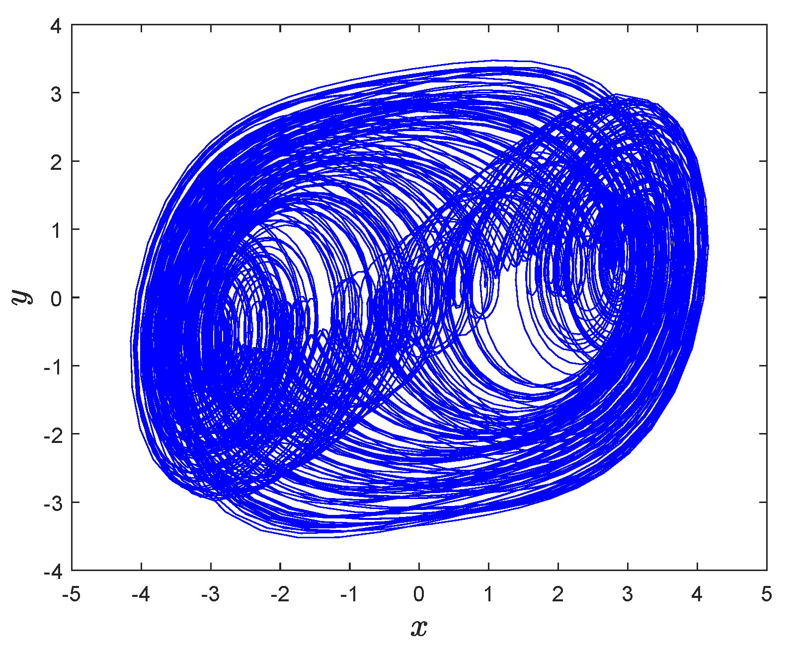
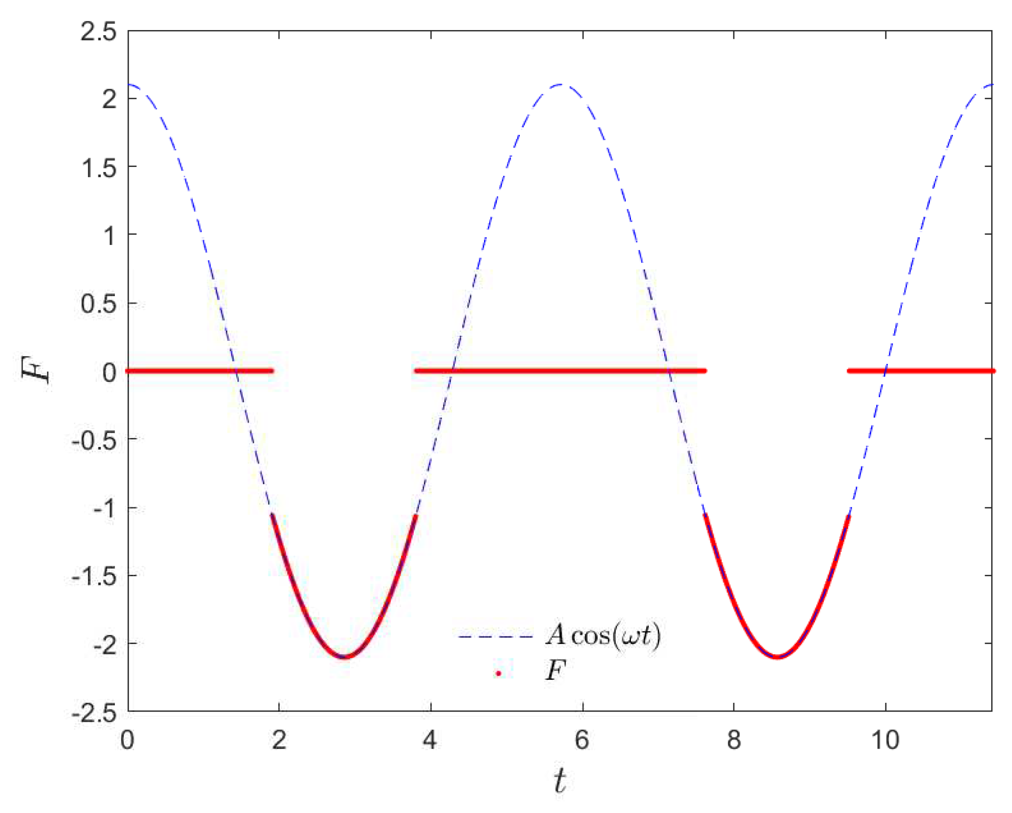
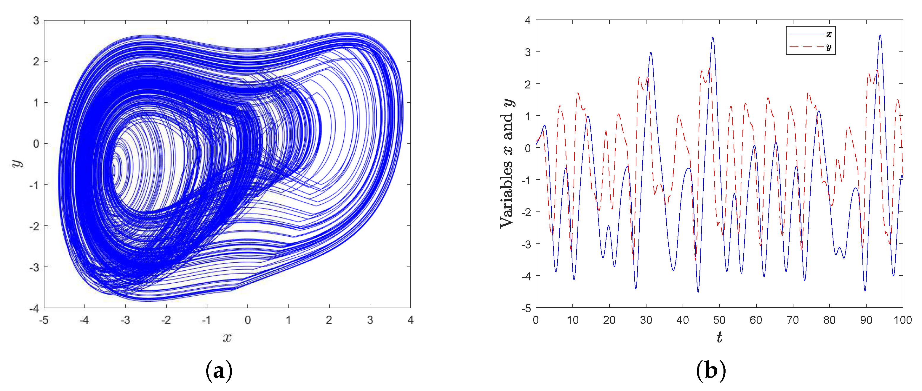
3.1. Design of MD System with Intermittent External Force

In order to investigate the dynamic characteristic for an MD system, an intermittent external force F of System (3) was designed, and it is given by

$$F=\left\{\begin{array}{ccc}Acos\omega t,\hfill & \hfill & \mathrm{if}t\in [t_i,t_i+\tau ]\subset [T_i,T_{i+1}],\hfill \\ 0,\hfill & \hfill & \mathrm{if}t\notin [t_i,t_i+\tau ]\subset [T_i,T_{i+1}],\hfill \end{array}\right.$$

(9)

where $[T_i,T_{i+1}](i=0,1,2,\cdots ,T_0=0)$ is a periodic interval, $\Delta T=T_{i+1}-T_i(i=0,1,2,\cdots )$, and $\tau$ is the length of control time in an interval $[T_i,T_{i+1}]$, i.e., the modified Duffing system can be expressed as

$$\left\{\begin{array}{ccc}\left\{\begin{array}{c}\dot{x}=-\beta x+y,\hfill \\ \dot{y}=k_{1}x-k_2{x}^3+Acoswt,\hfill \end{array}\right.\hfill & \hfill & \mathrm{if}t\in [t_i,t_i+\tau ]\subset [T_i,T_{i+1}],\hfill \\ \left\{\begin{array}{c}\dot{x}=-\beta x+y,\hfill \\ \dot{y}=k_{1}x-k_2{x}^3,\hfill \end{array}\right.\hfill & \hfill & \mathrm{if}t\notin [t_i,t_i+\tau ]\subset [T_i,T_{i+1}].\hfill \end{array}\right.$$

(10)

MD System (10) can also be called a switching system. When $t\in [t_i,t_i+\tau ]\subset [T_i,T_{i+1}]$, the external force of System (10) is working, i.e., $F=Acos\omega t$. It is at rest when $t\notin [t_i,t_i+\tau ]\subset [T_i,T_{i+1}]$, i.e., $F=0$.

3.2. Simulation Experiment of MD System with Intermittent External Force

If the initial values and parameters of MD System (10) are taken as

$$\left\{\begin{array}{c}(x_0,y_0,t_0)=(0.1,0.2,0),A=2.1,\omega =1.1,\hfill \\ \beta =0.2,k_1=0.6,k_2=0.1,\tau =\frac{2\pi }{3\omega },\hfill \\ [T_i,T_{i+1}]=\left[\frac{i·2\pi }{\omega },\frac{(i+1)·2\pi }{\omega }\right],t_i=\frac{i·2\pi +2\pi }{3\omega },(i=0,1,2,\cdots )\hfill \end{array}\right.$$

(11)

where the length of periodic time ${\displaystyle \Delta T=T_{i+1}-T_i=\frac{2\pi }{\omega }}$, then intermittent external force F is shown in Figure 2 (red line); the blue dotted line is continuous function $Acos\omega t$.

On the basis of Equation (10), the simulation experiments were implemented using Matlab software. Then, with the initial conditions in Equation (11), the chaotic attractor and diagram of variables $x\left(t\right)$ and $y\left(t\right)$ are shown in Figure 3a,b, respectively.

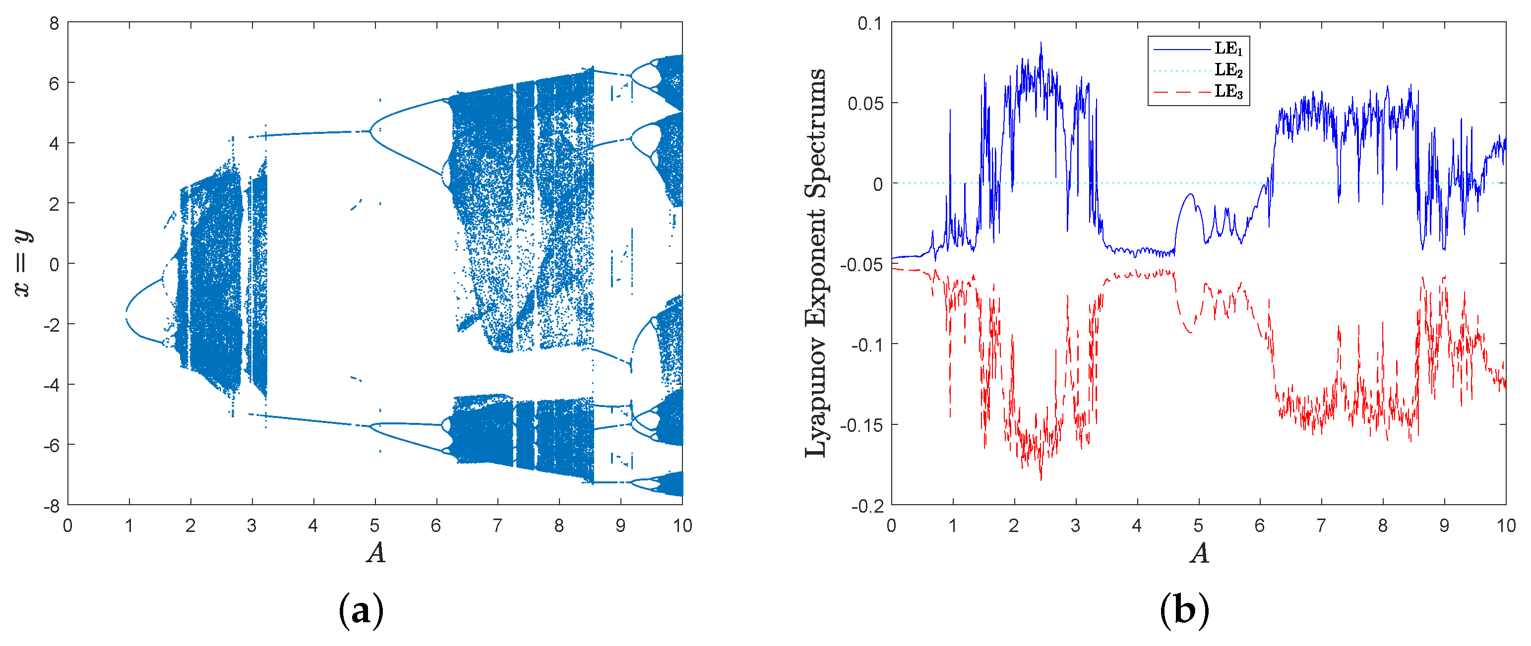
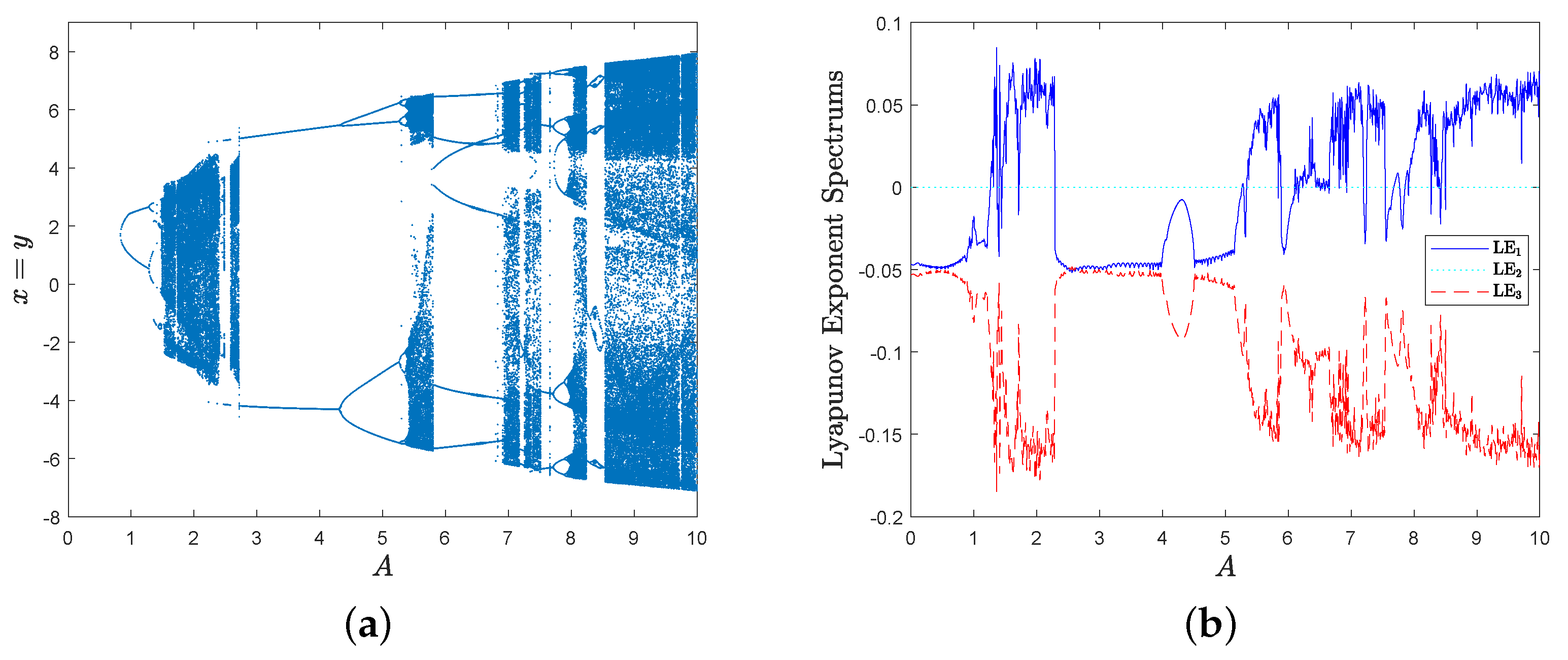
3.3. Dynamics Analysis of MD System with Respect to Parameter A

Chaotic systems are highly sensitive to their parameters. Different parameters lead the dynamic system to different states, such as periodic motion and chaotic motion. In order to know about the dynamic characteristics of an MD system, one needs to fix all parameters except for magnitude A of external force, i.e.,

$$\left\{\begin{array}{c}\beta =0.2,k_1=0.6,k_2=0.1,\omega =1.1,\tau =\frac{2\pi }{3\omega },A\in [0,10],\hfill \\ [T_i,T_{i+1}]=\left[\frac{i·2\pi }{\omega },\frac{(i+1)·2\pi }{\omega }\right],t_i=\frac{i·2\pi +2\pi }{3\omega },(i=0,1,2,\cdots ).\hfill \end{array}\right.$$

(12)

Then, the bifurcation diagram spectrum with respect to parameter A is given in Figure 4a, and the corresponding Lyapunov exponent spectrum with respect to parameter A is shown in Figure 4b.

Obviously, MD System (10) has a positive Lyapunov exponent in some parameter intervals, such as $[2.1,2.7]$, $[6.5,7.1]$ and $[7.8,8.5]$.

Furthermore, there are no positive Lyapunov exponents in interval $[3.5,6]$, i.e., one is equal to zero, and the others are negative; so, MD System (10) behaves periodically and there exists a limit cycle. For example, the phase diagram of MD System (10) is shown in Figure 5a when parameters $A=3.74$, and there exists a limit cycle when $t>500$. Similarly, MD System (10) behaves periodically too when $A=6$, and there exists a limit cycle in Figure 5b when $t>500$.

3.4. Dynamics Analysis of MD System with Respect to Parameter $\omega$

Similarly, if parameter $\omega$ is a variable and the others are fixed in MD System (10), i.e.,

$$\left\{\begin{array}{c}\beta =0.2,k_1=0.6,k_2=0.1,A=2.1,\tau =\frac{2\pi }{3\omega },\omega \in [0,2],\hfill \\ [T_i,T_{i+1}]=\left[\frac{i·2\pi }{\omega },\frac{(i+1)·2\pi }{\omega }\right],t_i=\frac{i·2\pi +2\pi }{3\omega },(i=0,1,2,\cdots ),\hfill \end{array}\right.$$

(13)

then the bifurcation diagram spectrum with respect to parameter $\omega$ and the corresponding Lyapunov exponent spectrum are shown in Figure 6a,b, respectively. MD System (10) has a positive Lyapunov exponent in parameter interval $[1,1.2]$.

3.5. Dynamics Analysis of MD System with Respect to Parameter $\tau$

Furthermore, if length of interval control time $\tau$ is a variable and the others are fixed, i.e.,

$$\left\{\begin{array}{c}\beta =0.2,k_1=0.6,k_2=0.1,A=2.1,\omega =1.1,\tau \in \left[0,\frac{4\pi }{3\omega }\right],\hfill \\ [T_i,T_{i+1}]=\left[\frac{i·2\pi }{\omega },\frac{(i+1)·2\pi }{\omega }\right],t_i=\frac{i·2\pi +2\pi }{3\omega },(i=0,1,2,\cdots ),\hfill \end{array}\right.$$

(14)

then the bifurcation diagram with respect to parameter $\tau$ and the corresponding Lyapunov exponent spectrum of MD System (10) are shown in Figure 7a,b. There are some parameter intervals in $\left[{\displaystyle 0,\frac{4\pi }{3w}}\right]$ that MD System (10) has a positive Lyapunov exponent, for example, it is chaotic in $\tau \in [1.7,3.2]$.

Note 1: If one considers replacing the original cosine function in Equation (9) with a constant, i.e., the intermittent external force is given by

$$F=\left\{\begin{array}{ccc}A,\hfill & \hfill & \mathrm{if}t\in [t_i,t_i+\tau ]\subset [T_i,T_{i+1}],\hfill \\ 0,\hfill & \hfill & \mathrm{if}t\notin [t_i,t_i+\tau ]\subset [T_i,T_{i+1}],\hfill \end{array}\right.$$

(15)

where $[T_i,T_{i+1}](i=0,1,2,\cdots ,T_0=0)$ is a periodic interval, $\Delta T=T_{i+1}-T_i(i=0,1,2,\cdots )$, and $\tau$ is the length of control time in an interval $[T_i,T_{i+1}]$, then the MD system can be expressed as

$$\left\{\begin{array}{ccc}\left\{\begin{array}{c}\dot{x}=-\beta x+y,\hfill \\ \dot{y}=k_{1}x-k_2{x}^3+A,\hfill \end{array}\right.\hfill & \hfill & \mathrm{if}t\in [t_i,t_i+\tau ]\subset [T_i,T_{i+1}],\hfill \\ \left\{\begin{array}{c}\dot{x}=-\beta x+y,\hfill \\ \dot{y}=k_{1}x-k_2{x}^3,\hfill \end{array}\right.\hfill & \hfill & \mathrm{if}t\notin [t_i,t_i+\tau ]\subset [T_i,T_{i+1}].\hfill \end{array}\right.$$

(16)

Similarly, the initial values and parameters of MD System (16) are taken as

$$\left\{\begin{array}{c}(x_0,y_0,t_0)=(0.1,0.2,0),A=2,\omega =1.1,\hfill \\ \beta =0.2,k_1=0.6,k_2=0.1,\tau =\frac{2\pi }{3\omega },\hfill \\ [T_i,T_{i+1}]=\left[\frac{i·2\pi }{\omega },\frac{(i+1)·2\pi }{\omega }\right],t_i=\frac{i·2\pi +2\pi }{3\omega },(i=0,1,2,\cdots )\hfill \end{array}\right.$$

(17)

where the length of a periodic time ${\displaystyle \Delta T=T_{i+1}-T_i=\frac{2\pi }{\omega }}$, then the attractor is given in Figure 8a, and the corresponding time-domain waveform is shown in Figure 8b.

In order to know about the dynamic characteristics of an MD system, one needs to fix all parameters except for magnitude A of external force, i.e.,

$$\left\{\begin{array}{c}\beta =0.2,k_1=0.6,k_2=0.1,\omega =1.1,\tau =\frac{2\pi }{3\omega },A\in [0,10],\hfill \\ [T_i,T_{i+1}]=\left[\frac{i·2\pi }{\omega },\frac{(i+1)·2\pi }{\omega }\right],t_i=\frac{i·2\pi +2\pi }{3\omega },(i=0,1,2,\cdots ).\hfill \end{array}\right.$$

(18)

Then, the bifurcation diagram with respect to parameter A is given in Figure 9a, and the corresponding Lyapunov exponent spectrum with respect to parameter A is shown in Figure 9b. Obviously, there also exists a positive Lyapunov exponent in some intervals, such as $[1.5,2.3]\cup [8.6,10]$.

4. Algorithm Design and Information-Encryption Application

In this section, an information-encryption algorithm was designed on the basis of the proposed MD system, and the corresponding experiment and security analysis are given.

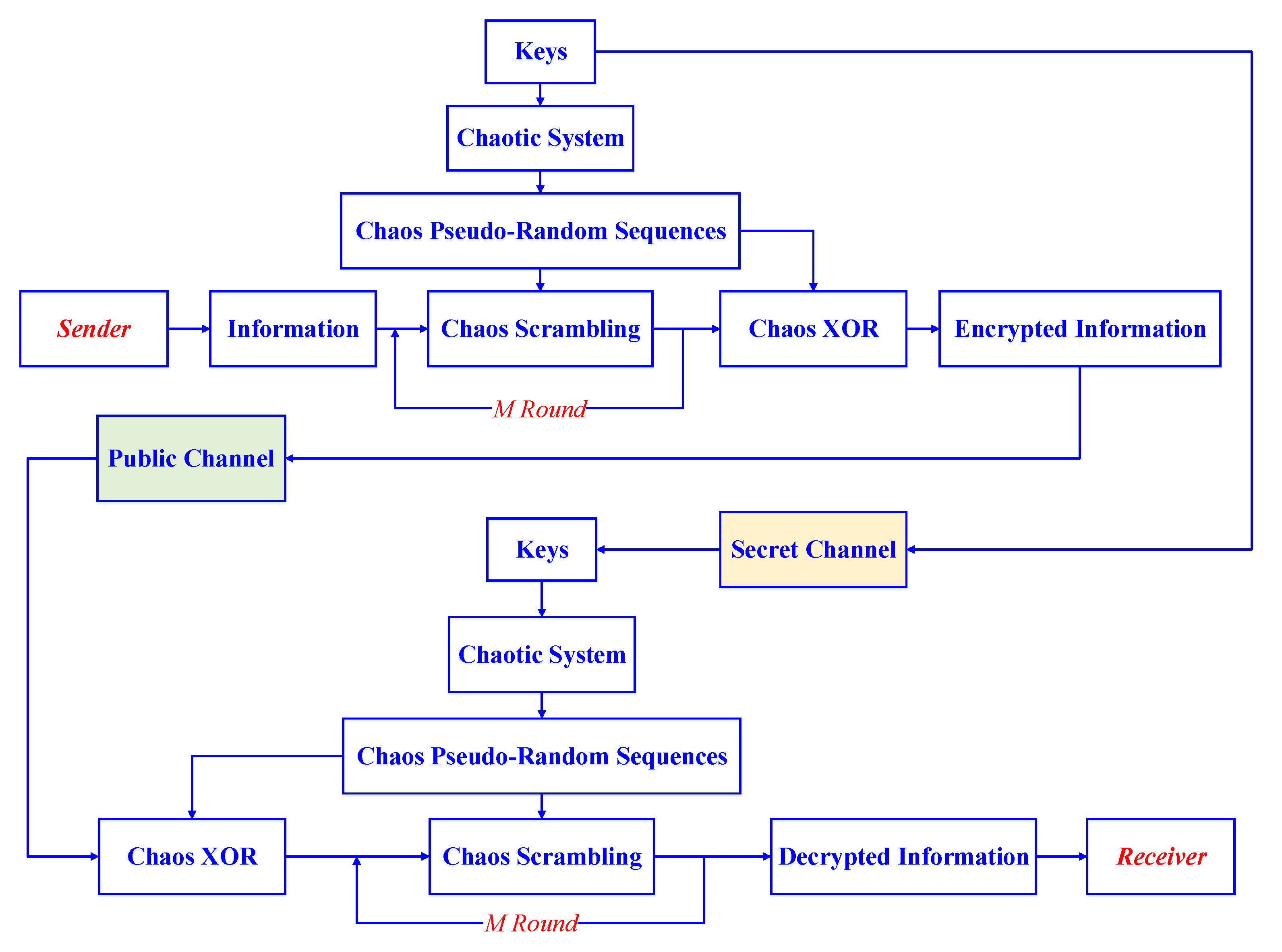
4.1. Algorithm Design

According to the MD system, a simple encryption algorithm is given, including scrambling encryption and chaos XOR encryption. First, the pseudorandom sequence was designed with the following steps.

Step 1: Generate pseudorandom sequence from MD system.

The fourth-order Runge–Kutta algorithm was used to solve MD System (10), and it is given by

$$\left\{\begin{array}{cc}\hfill {\mathit{X}}_{m+1}& ={\mathit{X}}_m+h·\frac{\left({\mathit{d}}_1+2{\mathit{d}}_2+2{\mathit{d}}_3+{\mathit{d}}_4\right)}{6},\hfill \\ \hfill {\mathit{d}}_1& =f\left(t_m,{\mathit{X}}_m\right),\hfill \\ \hfill {\mathit{d}}_2& =f\left(t_m+\frac{h}{2},{\mathit{X}}_m+h·\frac{{\mathit{d}}_1}{2}\right),\hfill \\ \hfill {\mathit{d}}_3& =f\left(t_m+\frac{h}{2},{\mathit{X}}_m+h·\frac{{\mathit{d}}_2}{2}\right),\hfill \\ \hfill {\mathit{d}}_4& =f\left(t_m+h,{\mathit{X}}_m+h·\frac{{\mathit{d}}_3}{2}\right),\hfill \end{array}\right.$$

(19)

where $\mathit{X}=[x,y]$, ${\mathit{X}}_m$ is the m-th value of variable $\mathit{X}$, h is the calculation step, and ${\mathit{d}}_1,{\mathit{d}}_2,{\mathit{d}}_3,{\mathit{d}}_4$ are the derivatives of $\dot{x}$ and $\dot{y}$ in Equation (10). If initial value ${\mathit{X}}_0=[x_0,y_0]$, step h, length of time T, and total iteration N are given, then one gets chaotic sequence $\mathit{X}=[x,y]$ in the length of N.

Step 2: Remove pseudorandom sequence in $\left[0,t_z\right]$ before the MD system enters the chaotic attractor, and obtain pseudorandom sequence ${\mathit{X}}_{[t_z,T]}$ after $t_z$.

Step 3: By moving the decimal point, removing integer parts, and taking absolute values, such as by multiplying the pseudorandom sequence by ${10}^{\theta }$ ($\theta$ is an integer), one gets

$$\begin{array}{c}\hfill {\mathit{S}}^{\theta }=\left|\mathrm{Floor}⌊\left({\mathit{X}}_{[t_z,T]}\times {10}^{\eta }-\mathrm{Floor}⌊{\mathit{X}}_{[t_z,T]}\times {10}^{\eta }⌋\right)\times {10}^{\theta }⌋\right|,\end{array}$$

(20)

where “Floor” is a function to take the integer part in the direction of negative infinity.

Step 4: Take a modular operation for pseudorandom sequence ${\mathit{S}}^{\theta }$ and convert it into binary sequence $\mathit{S}$, i.e.,

$$\begin{array}{c}\hfill \mathit{S}=\mathrm{Dec}2\mathrm{bin}\left(\mathrm{Mod}\left({\mathit{S}}^{\theta },2^{\gamma }\right)\right),\end{array}$$

(21)

where “Mod” is a modulus function, “Dec2bin” is a decimal-to-binary function, and $\gamma$ is an integer.

Encryption 1: Scrambling Encryption

Information is encrypted by the scrambling encryption based on preprocessed pseudorandom sequence ${\mathit{S}}^{\theta }$.

Sequences ${\mathit{S}}^{\theta }=[{\mathit{S}}_1^{\theta },{\mathit{S}}_2^{\theta }]$ are modeled by L (L is information length), and the new sequence or a pair of sequences is/are used as new position(s) to exchange the position of the original information, i.e., adjust the position of the original information as

$$\begin{array}{c}\hfill \mathit{I}\left(i\right)\leftrightarrow \mathit{I}\left({\mathit{S}}_1^{\theta }\right),\mathrm{or}\mathit{I}\left(i\right)\leftrightarrow \mathit{I}\left({\mathit{S}}_2^{\theta }\right),\mathrm{or}\mathit{I}(i,j)\leftrightarrow \mathit{I}({\mathit{S}}_1^{\theta },{\mathit{S}}_2^{\theta }),\end{array}$$

(22)

where $\mathit{I}\left(0\right)\leftrightarrow \mathit{I}(\mathrm{end})$, or $\mathit{I}(0,0)\leftrightarrow \mathit{I}(\mathrm{end},\mathrm{end})$.

Encryption 2: Chaos XOR Encryption

Transform information data $\mathit{I}$ into a binary sequence, and obtain encrypted information $\mathit{E}$ by

$$\begin{array}{c}\hfill \mathit{E}=\mathit{I}\oplus \mathit{S},\end{array}$$

(23)

where ⊕ is the operation of XOR.

On the receiving side, the decryption process is the inverse operation of above encryption algorithm, and the original information is successfully recovered with the correct keys.

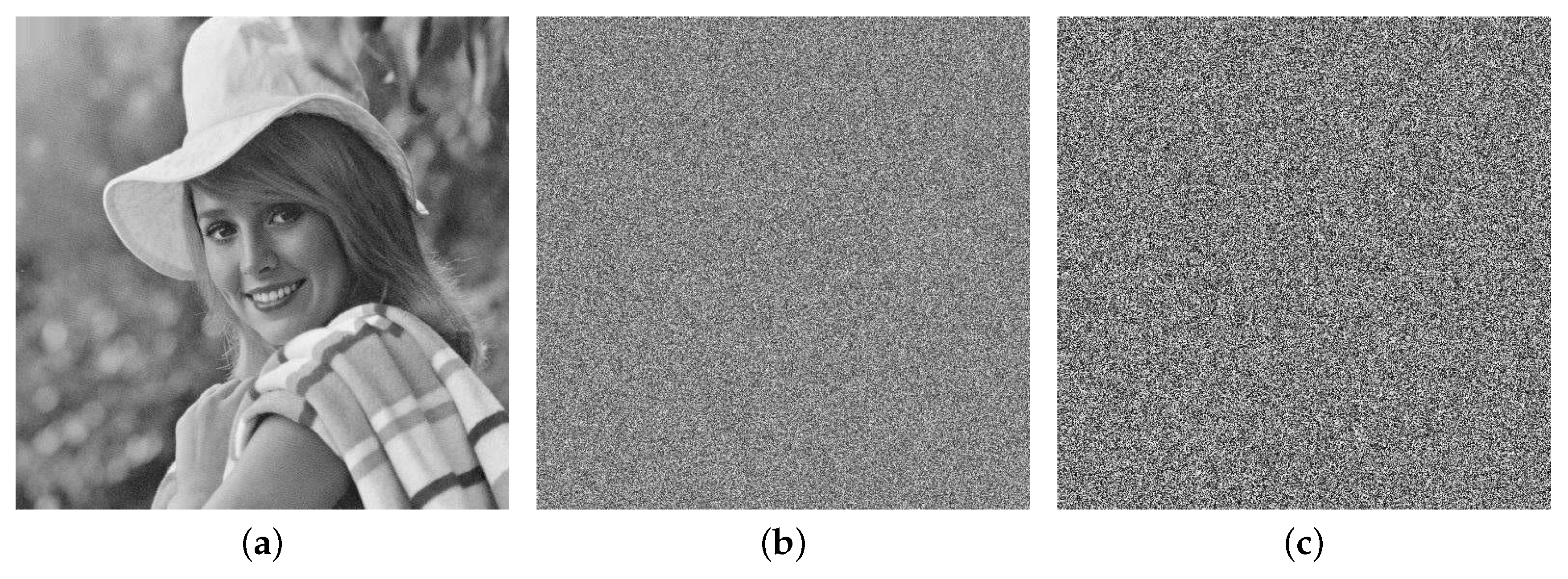
4.2. Simulation Experiment

By taking a gray image as an example, the simulation experiments of the encryption algorithm were verified with Matlab software. The flowchart of chaos-based secure communication is shown in Figure 10. On the sender side, the pseudorandom sequence is generated with the keys in the first, and original information is encrypted by the scrambling encryption in Encryption 1 for M rounds; then, it encrypted by the second chaos XOR encryption in Encryption 2. Therefore, the encrypted information is transmitted to the receiver via the public channel, and it is recovered by the inverse operations of encryption algorithm with the correct keys.

If initial conditions are

$$\left\{\begin{array}{c}(x_0,y_0,t_0)=(0.1,0.2,0),\omega =1.1,\hfill \\ \beta =0.2,k_1=0.6,k_2=0.1,A=2.1,\tau =\frac{2\pi }{3\omega },\eta =0,\hfill \\ T=500,h=0.001,\Delta T=2\pi /\omega ,\theta =12,\gamma =31,M=2,\hfill \\ t_i=\frac{i·2\pi +2\pi }{3\omega },[T_i,T_{i+1}]=\left[\frac{i·2\pi }{\omega },\frac{(i+1)·2\pi }{\omega }\right],(i=0,1,2,\cdots )\hfill \end{array}\right.$$

(24)

then the pseudorandom sequences are generated based on the MD system, and they are used to encrypt original image $\mathit{I}$ with the encryption algorithm. Simulation results are given in Figure 11, where Figure 11a is original image $\mathit{I}$, Figure 11b is encrypted image ${\mathit{E}}_1$ after two rounds of scrambling encryption, and Figure 11c is final encrypted image ${\mathit{E}}_2$ after chaos scrambling encryption and chaos XOR encryption. Obviously, it is difficult to obtain useful information from encrypted information.

In the receiver end, one can recover image I with the same initial conditions and parameters, and the recovered image is given in Figure 12c. However, it cannot be successfully recovered if one of the initial conditions or parameters is incorrect, and the corresponding experiment results are shown in Figure 12a,b.

4.3. Key Sensitivity and Key Space

Key sensitivity was tested by initial conditions with small error. If we let

$$\left\{\begin{array}{c}(x_0^{\prime },y_0,t_0)=(0.1000000000000001,0.2,0),\omega =1.1,\hfill \\ \beta =0.2,k_1=0.6,k_2=0.1,A=2.1,\tau =\frac{2\pi }{3\omega },\eta =0,\hfill \\ T=500,h=0.001,\Delta T=2\pi /\omega ,\theta =12,\gamma =31,M=2,\hfill \\ t_i=\frac{i·2\pi +2\pi }{3\omega },[T_i,T_{i+1}]=\left[\frac{i·2\pi }{\omega },\frac{(i+1)·2\pi }{\omega }\right],(i=0,1,2,\cdots )\hfill \end{array}\right.$$

(25)

i.e., error of initial variable $x_0$ is ${10}^{-16}$, then the decryption image is shown in Figure 12a. Similarly, if we let

$$\left\{\begin{array}{c}{\omega }^{\prime }=1.100000000000001,(x_0,y_0,t_0)=(0.1,0.2,0),\hfill \\ \beta =0.2,k_1=0.6,k_2=0.1,A=2.1,\tau =\frac{2\pi }{3\omega },\eta =0,\hfill \\ T=500,h=0.001,\Delta T=2\pi /\omega ,\theta =12,\gamma =31,M=2,\hfill \\ t_i=\frac{i·2\pi +2\pi }{3\omega },[T_i,T_{i+1}]=\left[\frac{i·2\pi }{\omega },\frac{(i+1)·2\pi }{\omega }\right],(i=0,1,2,\cdots )\hfill \end{array}\right.$$

(26)

i.e., error of initial parameter $\omega$ is ${10}^{-15}$, then the decrypted image is shown in Figure 12b. Some initial conditions were tested and the results are given in

Table 1. Test results of recovered image with a parameter error of initial conditions.

One Parameter Error of Initial Conditions	Whether Original Image Recovered Successfully or Not	One Parameter Error of Initial Conditions	Whether Original Image Recovered Successfully or Not
$\left|x_0-x_0^{\prime }\right|⩾{10}^{-16}$	No	$\left|w-w^{\prime }\right|⩾{10}^{-15}$	No
$\left|y_0-y_0^{\prime }\right|⩾{10}^{-16}$	No	$\left|k_1-k_1^{\prime }\right|⩾{10}^{-16}$	No
$\left|t_0-t_0^{\prime }\right|⩾{10}^{-17}$	No	$\left|k_2-k_2^{\prime }\right|⩾{10}^{-16}$	No
$\left|\beta -{\beta }^{\prime }\right|⩾{10}^{-16}$	No	$\left|A-A^{\prime }\right|⩾{10}^{-15}$	No

. So, key-space (KS) size can be estimated from the above key-sensitivity accuracy, i.e.,

$$\begin{array}{c}\hfill \mathrm{KS}⩾{10}^{16}\times {10}^{16}\times {10}^{17}\times {10}^{16}\times {10}^{15}\times {10}^{16}\times {10}^{16}\times {10}^{15}={10}^{127}=2^{422}.\end{array}$$

(27)

4.4. NIST Test

NIST tests may be useful as a first step in determining whether or not a generator is suitable for a particular cryptographic application. For sequences generated from chaotic systems, NIST tests provide a necessary randomness test by probabilistic methods. If the test results of p-values are greater than a significance level of 0.01, then it indicates that the sequence from the generator is random [43]. For sequence $\mathit{S}=\mathrm{Dec}2\mathrm{bin}\left(\mathrm{Mod}\left({\mathit{S}}^{\theta },2^{31}\right)\right)$ generated from the MD system, with a size greater than ${10}^8$ bit binary data, test results are given in

Table 2. NIST test results.

Statistical Tests	p-Value
Frequency	0.5341
Block frequency	0.1453
Cumulative sums	0.6082
Runs	0.1626
Longest run	0.6163
Rank	0.8514
FFT	0.9915
Nonoverlapping templates	0.4491
Overlapping templates	0.9114
Universal	0.9558
Approximate entropy	0.4944
Random excursions	0.4273
Random excursions variant	0.9982
Linear complexity	0.4166
Serial	0.8513
Success	All

. Obviously, p-Values were greater than 0.01, and it passed all NIST tests.

5. Conclusions

On the basis of the Duffing oscillator, an MD chaotic system with intermittent external force was investigated. The Lyapunov exponent spectra and bifurcation diagrams spectra were given to depict the dynamic characteristics of an MD system, and it behaved as a chaotic attractor in some parameter intervals. Meanwhile, through the pseudorandom sequence of MD system, an encryption algorithm consisting of chaos-scrambling encryption and chaos XOR encryption was designed. Simulation experiments showed its feasibility and validity via image encryption. Security analysis showed that the algorithm could pass the NIST test and that it is highly sensitive to initial conditions and parameters. The proposed MD system could be applied to the design of new chaotic systems and chaos-based encryption algorithms in the future.

References

1. Kolen, M.J. The Duffing Equation—Nonlinear Oscillators and Their Behaviour; John Wiley & Sons, Ltd.: West Sussex, UK, 2011; pp. 1–63. ISBN 9780470977835. [Google Scholar]
2. Chen, G.R.; Ueta, T. Yet another chaotic attractor. Int. J. Bifurcat. Chaos 1999, 9, 1465–1466. [Google Scholar] [CrossRef]
3. Lü, J.H.; Chen, G.R. A new chaotic attractor coined. Int. J. Bifurcat. Chaos 2002, 12, 659–661. [Google Scholar] [CrossRef]
4. Chen, Q.G.; Chen, G.R. A chaotic system with one saddle and two stable node-foci. Int. J. Bifurcat. Chaos 2008, 18, 1393–1414. [Google Scholar]
5. Yang, Q.G.; Wei, Z.C.; Chen, G.R. An unusual 3D autonomous quadratic chaotic system with two stable nodefoci. Int. J. Bifurcat. Chaos 2010, 20, 1061–1083. [Google Scholar] [CrossRef]
6. Novak, S.; Frehlich, R.G. Transition to chaos in the Duffing oscillator. Phys. Rev. A 1982, 26, 3660–3663. [Google Scholar] [CrossRef]
7. Vincent, U.E.; Kenfack, A. Synchronization and bifurcation structures in coupled periodically forced non-identical Duffing oscillators. Phys. Scripta 2008, 77, 045005. [Google Scholar] [CrossRef]
8. Chabreyrie, R.; Aubry, N. Switching chaos on/off in Duffing oscillator. arXiv 2011, arXiv:1108.4118. [Google Scholar]
9. Kozlowski, J.; Parlitz, U.; Lauterborn, W. Bifurcation analysis of two coupled periodically driven Duffing oscillators. Phys. Rev. E 1995, 51, 1861–1867. [Google Scholar] [CrossRef]
10. Sabarathinam, S.; Volos, C.K.; Thamilmaran, K. Implementation and study of the nonlinear dynamics of a memristor-based duffing oscillator. Nonlinear Dyn. 2017, 87, 37–49. [Google Scholar] [CrossRef]
11. Niknam, A.; Farhang, K. Friction-induced vibration in a two-mass damped system. J. Sound Vibrat. 2019, 456, 454–475. [Google Scholar] [CrossRef]
12. Li, C.; Sprott, J.C.; Yuan, Z.; Li, H. Constructing chaotic systems with total amplitude control. Int. J. Bifurcat. Chaos 2015, 25, 1530025. [Google Scholar] [CrossRef]
13. Yu, S.M.; Tang, W.K.S.; Lü, J.H.; Chen, G.R. Generation of n × m-wing Lorenz-like attractors from a modified Shimizu-Morioka model. IEEE Trans. Circuits Syst.-II 2008, 55, 1168–1172. [Google Scholar] [CrossRef]
14. Pham, V.-T.; Jafari, S.; Wang, X.; Ma, J. A chaotic system with different shapes of equilibria. Int. J. Bifurcat. Chaos 2016, 26, 1650069. [Google Scholar] [CrossRef]
15. Zhang, F.C.; Liao, X.F.; Zhang, G.Y. Qualitative behaviors of the continuous-time chaotic dynamical systems describing the interaction of waves in plasma. Nonlinear Dyn. 2017, 88, 1623–1629. [Google Scholar] [CrossRef]
16. Sun, J.; Lu, C.; Yuan, X. Lagrange stability for impulsive Duffing equations. J. Diff. Equ. 2019, 266, 6924–6962. [Google Scholar]
17. Varshney, V.; Sabarathinam, S.; Prasad, A.; Thamilmaran, K. Infinite number of hidden attractors in memristor-based autonomous duffing oscillator. Int. J. Bifurcat. Chaos 2018, 28, 1850013. [Google Scholar] [CrossRef]
18. Vaidyanathan, S. Anti-synchronization of Duffing double-well chaotic oscillators via integral sliding mode control. Int. J. ChemTech Res. 2016, 9, 297–304. [Google Scholar]
19. Kabziński, J. Synchronization of an uncertain Duffing oscillator with higher order chaotic systems. Int. J. Appl. Math. Comput. Sci. 2018, 28, 625–634. [Google Scholar] [CrossRef]
20. Wang, X.; Pham, V.-T.; Volos, C. Dynamics, circuit design, and synchronization of a new chaotic system with closed curve equilibrium. Complexity 2017, 2017, 7138971. [Google Scholar] [CrossRef]
21. Pham, V.-T.; Jafari, S.; Volos, C.; Giakoumis, A.; Vaidyanathan, S.; Kapitaniak, T. A chaotic system with equilibria located on the rounded square loop and its circuit implementation. IEEE Trans. Circuits Syst.-II 2016, 63, 878–882. [Google Scholar] [CrossRef]
22. Li, C.; Xu, X.; Ding, Y.; Dou, B. Weak photoacoustic signal detection based on the differential Duffing oscillator. Int. J. Modern Phys. B 2018, 32, 1850103. [Google Scholar] [CrossRef]
23. Wang, G.; He, S. A quantitative study on detection and estimation of weak signals by using chaotic Duffing oscillators. IEEE Trans. Circuits Syst.-I 2003, 50, 945–953. [Google Scholar] [CrossRef]
24. Li, C.; Luo, G.; Li, C. A parallel image encryption algorithm based on chaotic Duffing oscillators. Multimedia Tools Appl. 2018, 77, 19193–19208. [Google Scholar] [CrossRef]
25. Zapateiro, M.; Vidal, Y.; Acho, L. A secure communication scheme based on chaotic duffing oscillators and frequency estimation for the transmission of binary-coded messages. Communicat. Nonlinear Sci. Numer. Simul. 2014, 19, 991–1003. [Google Scholar] [CrossRef]
26. Nicolis, C. Climatic responses to systematic time variations of parameters: A dynamical approach. Nonlin. Processes Geophys. 2018, 25, 649–658. [Google Scholar] [CrossRef]
27. Nicolis, C. Self-oscillations and predictability in climate dynamics. Tellus 1984, 36, 1–10. [Google Scholar] [CrossRef]
28. Nicolis, C. Irreversible thermodynamics of a simple atmospheric flow model. Int. J. Bifurcation Chaos 2002, 12, 2557–2566. [Google Scholar] [CrossRef]
29. Kwasniok, F. Analysis and modelling of glacial climate transitions using simple dynamical systems. Philos. Trans. Math. Phys. Eng. Sci. 2013, 371, 1–22. [Google Scholar] [CrossRef]
30. Nicolis, G.; Nicolis, C. Stochastic resonance, self-organization and information dynamics in multistable systems. Entropy 2016, 18, 172. [Google Scholar] [CrossRef]
31. Zaher, A.A. Duffing oscillators for secure communication. Comput. Electr. Eng. 2018, 71, 77–92. [Google Scholar] [CrossRef]
32. Chen, G.R.; Mao, Y.B.; Chui, C.K. A symmetric image encryption scheme based on 3D chaotic cat maps. Chaos Solit. Fract. 2004, 21, 749–761. [Google Scholar] [CrossRef]
33. Kwok, H.S.; Tang, W.K.S. A fast image encryption system based on chaotic maps with finite precision representation. Chaos Solit. Fract. 2007, 32, 1518–1529. [Google Scholar] [CrossRef]
34. Liu, X.; Song, Y.; Jiang, G.P. Hierarchical bit-level image encryption based on chaotic map and feistel network. Int. J. Bifurcat. Chaos 2019, 29, 1950016. [Google Scholar] [CrossRef]
35. Preishuber, M.; Hütter, T.; Katzenbeisser, S.; Uhl, A. Depreciating motivation and empirical security analysis of chaos-based image and video encryption. IEEE Trans. Informat. Forensics Secur. 2018, 13, 2137–2150. [Google Scholar] [CrossRef]
36. He, J.; Yu, S.; Cai, J. Topological horseshoe analysis for a three-dimensional anti-control system and its application. Optik 2016, 127, 9444–9456. [Google Scholar] [CrossRef]
37. Zhang, Y.Q.; Wang, X.Y. Analysis and improvement of a chaos-based symmetric image encryption scheme using a bit-level permutation. Nonlinear Dyn. 2014, 77, 687–698. [Google Scholar] [CrossRef]
38. Wang, X.Y.; Li, P.; Zhang, Y.Q.; Liu, L.Y.; Zhang, H.; Wang, X. A novel color image encryption scheme using dna permutation based on the lorenz system. Multimedia Tools Appl. 2017, 77, 6243–6265. [Google Scholar] [CrossRef]
39. Ashwin, P.; Camp, C.; Von der Heydt, A. Chaotic and non-chaotic response to quasiperiodic forcing: Limits to predictability of ice ages paced by Milankovitch forcing. Dyn. Stat. Clim. Syst. 2018, 3, 1–30. [Google Scholar]
40. Li, C.; Feng, B.; Li, S.; Kurths, J.; Chen, G. Dynamic analysis of digital chaotic maps via state-mapping networks. IEEE Trans. Circuits Syst.-I 2019, 66, 2322–2335. [Google Scholar] [CrossRef]
41. Li, C.; Zhang, Y.; Xie, E.Y. When an attacker meets a cipher-image in 2018: A year in review. J. Inf. Security Appl. 2019, 48, 102361. [Google Scholar] [CrossRef]
42. He, J.; Cai, J. Design of a new chaotic system based on Van der Pol oscillator and its encryption application. Mathematics 2019, 7, 743. [Google Scholar] [CrossRef]
43. Murillo-Escobar, M.A.; Cruz-Hernndez, C.; Cardoza-Avendaño, L.; Méndez-Ramrez, R. A novel pseudorandom number generator based on pseudorandomly enhanced logistic map. Nonlinear Dyn. 2017, 87, 407–425. [Google Scholar] [CrossRef]
Figure 1. Chaotic attractor of System (3) with parameters in Equation (4).
Applsci 09 04683 g001
Figure 2. Intermittent external force F (red) of modified Duffing (MD) System (10) and continuous function A cos ω t (dotted line).
Applsci 09 04683 g002
Figure 3. (a) Chaotic attractor of MD system (10). (b) Time-domain waveform of variables x ( t ) and y ( t ) when initial conditions are given in Equation (11).
Applsci 09 04683 g003
Figure 4. (a) Bifurcation diagram with respect to parameter A of Poincare cross-section of MD system (10) when x = y and t > 500 . (b) Lyapunov exponent spectrum with respect to parameter A of MD System (10) when the other parameters are given in Equation (12).
Applsci 09 04683 g004
Figure 5. (a) Limit cycle of MD System (10) when A = 3.74 and t > 500 . (b) Limit cycle of MD System (10) when A = 6 and t > 500 .
Applsci 09 04683 g005
Figure 6. (a) Bifurcation diagram with respect to parameter ω of Poincare cross-section of MD System (10) when x = y and t > 500 . (b) Lyapunov exponent spectra with respect to parameter ω of MD System (10) when other parameters are given in Equation (13).
Applsci 09 04683 g006
Figure 7. (a) Bifurcation diagram with respect to parameter τ of Poincare cross-section of MD System (10) when x = y and t > 500 . (b) Lyapunov exponent spectra with respect to parameter τ when other parameters are given in Equation (14).
Applsci 09 04683 g007
Figure 8. (a) Chaotic attractor of MD System (16). (b) Corresponding time-domain waveform of MD System (16).
Applsci 09 04683 g008
Figure 9. (a) Bifurcation diagram with respect to parameter A of Poincare cross-section of MD System (16) when x = y and t > 500 . (b) Lyapunov exponent spectra with respect to parameter A of MD System (16) when other parameters given in Equation (18).
Applsci 09 04683 g009
Figure 10. Flowchart of secure chaos-based communication.
Applsci 09 04683 g010
Figure 11. (a) Original image I . (b) Encrypted image E 1 after Encryption 1 (scrambling encryption), i.e., original image in (a) is encrypted only after two rounds of chaos scrambling encryption. (c) Encrypted image E 2 after Encryption 2 (chaos XOR encryption), i.e., image in (b) is again encrypted by chaos XOR encryption.
Applsci 09 04683 g011
Figure 12. (a) Recovered image with initial conditions given in Equation (25). (b) Recovered image with initial conditions given in Equation (26). (c) Recovered image with correct values of initial conditions and parameters.
Applsci 09 04683 g012