Abstract
In recent years, within large cities with a high population density, traffic congestion has become more and more serious, resulting in increased emissions of vehicles and reducing the efficiency of urban operations. Many factors have caused traffic congestion, such as insufficient road capacity, high vehicle density, poor urban traffic planning and inconsistent traffic light cycle configuration. Among these factors, the problems of traffic light cycle configuration are the focal points of this paper. If traffic lights can adjust the cycle dynamically with traffic data, it will reduce degrees of traffic congestion significantly. Therefore, a modified mechanism based on Q-Learning to optimize traffic light cycle configuration is proposed to obtain lower average vehicle delay time, while keeping significantly fewer processing steps. The experimental results will show that the number of processing steps of this proposed mechanism is 11.76 times fewer than that of the exhaustive search scheme, and also that the average vehicle delay is only slightly lower than that of the exhaustive search scheme by 5.4%. Therefore the proposed modified Q-learning mechanism will be capable of reducing the degrees of traffic congestions effectively by minimizing processing steps.
1. Introduction
In the past decade, world population has increased rapidly. Cities with high population density are inevitably facing problems of traffic congestion, inclusive of reducing commuting efficiency, worsening vehicle emissions, and increasing traffic accidents. Taiwan is one of the countries with the highest population density, and her capital, Taipei, is the city with the highest population density. Taipei has been affected by a large number of traffic and insensitive traffic lights during rush hours, causing serious traffic congestion problems.
Existing traffic lights are usually configured with a fixed cycle, and do not take into account specific traffic conditions. Such a configuration is very inefficient. When a large event is held during rush hours, it inevitably gives rise to traffic congestions. In the past, in order to solve these problems of traffic congestion, traffic officers could help relieve traffic congestion. However, this approach would lead to an increased manpower burden and cause unnecessary risk to these traffic officers. Thus, to solve traffic congestion problems, this paper proposes an intelligent traffic light system to initiate a better traffic light cycle configuration and to simulate the schemes by which traffic officers control traffic lights by analyzing the historical data. To achieve this system, a smart system is needed to adjust the cycle configuration of traffic lights by applying reinforcement learning [1,2,3] in machine learning [4].
It is an interesting topic to use information technology to solve traffic problems. For example, Jianbin Chen et al. [5] used the local space-time autoregressive (LSTAR) model to predict traffic flow, and a new parameter estimation method was formulated, based on the Localized Space-Time ARIMA (LSTARIMA) model to reduce computational complexity for real-time prediction purposes. It is noted that the new parameters estimation method of LSTARIMA uses a time variant weight matrix to improve traffic prediction accuracy. Peng Qin et al. [6] used image analysis to solve traffic problems. It is generally not possible to obtain a top view of intersections in real time, so we use past historical data with Modified Q-learning to solve traffic congestion problems. The dataset used in this paper was taken from the Department of Transportation, Taipei City Government. This data can collect traffic data through vehicle detectors [7], including traffic flow, steering ratio, number of lanes and road types. This study focuses on three important congestion intersections: The intersection of Minsheng W. Rd. and Huanhe N. Rd., the intersection of Nanjing W. Rd. and Huanhe N. Rd. and the intersection of Minsheng W. Rd. and Yanping N. Rd. These important intersections connect Taipei City and New Taipei City. These intersections have long been plagued by traffic congestion problems. We use modified Q-Learning to find better traffic light cycle configurations. The experimental results show that the model can effectively recommend a better traffic light cycle configuration.
2. Related Works
In recent years, the rapid development of artificial intelligence [8] technology, coupled with traffic road perception technology [9], has become quite mature. Therefore, the application of artificial intelligence and transportation can develop rapidly. Traffic road perception devices are capable of collecting various data in traffic, including traffic flow, steering ratios, number of lanes, road types and vehicle types. Machine learning is characterized by the ability to use collected data to train high-performance models. One of the most commonly-used ones is deep learning in machine learning, which can be classified into several categories, such as supervised learning, unsupervised learning and reinforcement learning, as shown in Figure 1. It should be noted that machine learning is a subset of artificial intelligence, and deep learning is a subset of machine learning.
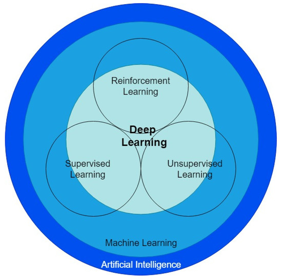
Figure 1.
The classification of artificial intelligence related technologies.
The reinforcement learning method, one of the machine learning methods, has achieved many outstanding results in interactive games. One of the most famous examples is AlphaGo [10], using deep learning combined with reinforcement learning to enable machines to transcend humans in the field of Go. This inspires the design of traffic light cycle configuration using the reinforcement learning schemes, such as Q-learning, regarding the interaction of traffic lights and machines. Q-learning is a model-free reinforcement learning algorithm, so it can handle problems using stochastic (random) transitions and rewards. That is, it can learn a policy and assign an agent to take actions under certain conditions, without requiring pre-defined adaptations. In this paper, we design a modified Q-Learning mechanism which optimizes traffic light period configuration to find the minimum average vehicle delay time (AVDT).
2.1. Intelligent Transportation System
The Intelligent Transportation System (ITS) is an integrated transportation management system that uses new technologies effectively for the entire transportation management system to make traffic safe, timely, accurate and efficient. In ITS, data can be obtained from a variety of sources, such as Vehicle Detector, GPS, Infrastructure sensors and camera detectors. As to the rapid development of ITS, Li Zhu et al. [11] proposed a guideline for the utilization of big data in modern ITS, including road traffic accidents analysis, road traffic flow prediction, and so on. Regarding the road traffic accidents analysis, Liang Qi et al. presented a system [12] that uses deterministic and stochastic Petri nets to design an emergency traffic-light control system. The system provided emergency responses to the intersections with accidents. For the aspect of road traffic flow prediction, D. Chen [13] proposed an improved artificial bee colony (ABC) algorithm that used the crossover and mutation operators of the differential evolution algorithm to replace the search strategy of employed bees in the ABC algorithm. Their research came out with an optimal road traffic flow prediction. In recent years, the technology applications and extensive applications of ITS have effectively handled License Plate Detection [14], parking guidance system [15], predicting driver’s activity [16] and other applications. Li, H. et al. [14] designed a novel architecture, named Roadside Parking net (RPnet), to accomplish license plate (LP) detection and recognition with high system accuracy and low processing time. Zhang, X., et al. [15] designed the Intelligent Travel and Parking Guidance System based on the A* algorithm to get the optimal routes. Through the system implementation, traffic delays were reduced, and traffic congestions were alleviated in their defined road network. Rekabdar, B. et al. [16] proposed the Dilated Convolutional Neural Network (DCNN) to classify driver’s actions and activities in real-world scenarios. Their proposed model functioned with less hand-picking features and high predicting precision.
2.2. Artificial Intelligence
Artificial intelligence (AI) refers to the wisdom expressed by the machines which have been made by people. It usually represents the technology of presenting human intelligence by using ordinary computer programs. AI applications include constructing an ability of reasoning, knowing, planning, learning, communicating, perceiving, moving objects, using tools and manipulating machinery, etc. Many tools are used in AI, consisting of versions of search and artificial neural networks (ANNs), mathematical optimization and methods based on statistics, probability and economics. Besides, AI constitutes a kind of interdisciplinary assimilation of computer science, information engineering, linguistics, psychology, mathematics and many other fields.
The rapid development of hardware devices has directly and indirectly helped AI development, and has surpassed humans in many fields, such as machine vision [17,18], natural language processing [19], games [20] and predictive classification, etc. These are all classified in machine learning.
2.3. Machine Learning
Machine learning is a branch of AI, and is a way to achieve this AI; that is, to solve problems in AI by using machine learning. Machine learning algorithms build mathematical models based on sample data (called training data) to make predictions or decisions without explicit programming to perform tasks. Machine learning has developed rapidly and diversely in recent years, involving many disciplines, such as probability theory, statistics, approximation theory, convex analysis and computational complexity theory.
Machine learning can be divided into three categories: Supervised learning [21], unsupervised learning [22] and reinforcement learning. The supervised learning algorithm is based on the budget to access the desired output of the limited input (training tag), and optimizes the selection of the input it receives for the training tag. In unsupervised learning, the algorithm builds a mathematical model from a set of data containing only inputs, but no desired output tags. The difference between supervised learning and unsupervised learning is whether the training set target has a label. Reinforcement learning deals with the interaction between the environment and the agent. In this paper, our model is based upon the reinforcement learning mechanism.
2.4. Reinforcement Learning
Reinforcement learning is a machine learning method based on Markov Decision Processes (MDP) [23]. Figure 2 shows a typical process flow of Markov Decision Processes. MDP is a discrete time stochastic control process, which is useful for studying optimization problems solved via dynamic programming and reinforcement learning. Reinforcement learning emphasizes the interaction between the agent and the environment, and gets the maximum expected reward from it. The difference between reinforcement learning and standard supervised learning is that it does not require the correct input and output pairs, nor does it require any precise correction of suboptimal behavior. There are well-known results in many fields, such as Cybernetics, Game Theory, and so on.
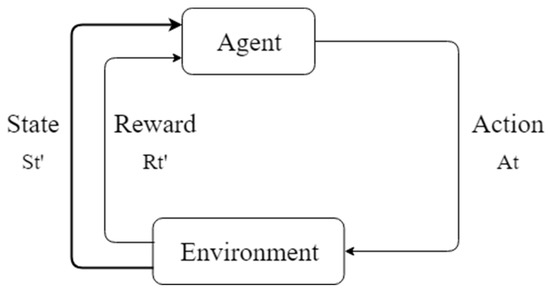
Figure 2.
Process flow of Markov Decision Processes (MDPs).
Reinforced learning has been used in traffic light configuration to help us find the best state by rewarding the actions chosen by the agent. Common methods of Reinforcement Learning are Q-learning [24,25], Sarsa [26,27] and Policy Gradients [28,29]. Among them, Q-learning is a prominent method in the field of control, which can reduce the risks and burdens caused by manual control.
2.5. Q-Learning
This Q-learning mechanism does not need to model the environment without special changes, even for transfer functions or reward functions with random factors. Q-learning is to record learned policies through a Q-table, and instructs the agent which action to take in order to gain the greatest reward value. It can lead to a policy that maximizes the reward expectations of all steps in a limited process. This article uses Q-learning and traffic lights interaction to learn and record vehicle delay time in each case to help the system find the maximum reward policy.
2.6. Vehicle Detector
Vehicle detectors can detect vehicles passing or arriving at a certain point, and are used to collect traffic information on roads, including traffic flow, steering ratio, number of lanes, road types and vehicle types. Most of detection methods are static. Some detectors are buried under the road through sensing elements. When a vehicle passes by, the magnetic field changes, and the information is obtained. Another way is to obtain traffic information by setting up infrared, Microwave or Ultrasonic sensors on the roadside. Alternatively, we can obtain traffic data by comparing traffic images at intersections with preset cameras.
2.7. Traffic Simulation System
The traffic simulation system is composed of highly complex mathematical models. It can calculate average vehicle delay time by traffic flow, traffic light cycle, road type and the number of lanes. It helps us simulate the control of traffic lights without having to directly control the actual traffic lights. It reduces the risk in actual operations.
3. Traffic Light Cycle Recommendation Methods
The data set [30] used in this paper was taken from the Department of Transportation, Taipei City Government. The data was collected during the rush hour periods from 7:00 to 9:00 and 17:00 to 19:00. Vehicle detectors can be used to collect traffic data, including traffic flow, steering ratio, number of lanes and road type. Figure 3 shows three of the most crowded intersections (Red mark: The intersection of Huanhe N. Rd. and Minsheng W. Rd.; Blue mark: The intersection of Huanhe N. Rd. and Nanjing W. Rd.; Green mark: The intersection of Yanping N. Rd. and Minsheng W. Rd.) in Taipei City. This study uses the modified Q-Learning method to find a better traffic light configuration cycle. The experimental environment is developed by the Taiwan Institute of Transportation, Taiwan Highway Capacity Software [31]. The system is dedicated to the Taiwan road analysis, and is set differently for different states in each region.
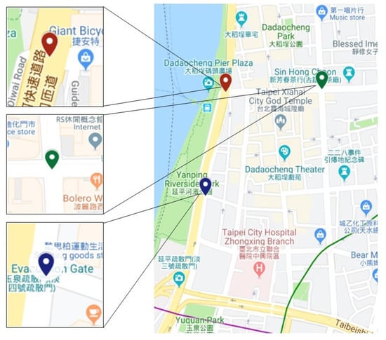
Figure 3.
Crowded intersections in Taipei City.
3.1. Road Traffic Indicator
Traffic congestion is a complicated problem [11]. There are many parameters needed to be considered, such as the Saturation Flow Rate of the intersection, Lane Capacity, Effective Green Light of the Saturation Flow Rate, Degree of Saturation and Average Vehicle Delay Time (AVDT). These data can be calculated by the following methods.
Saturation Flow Rate, S, refers to the number of vehicles that pass through an intersection within one hour, and is often used to evaluate the throughput of the lane. The calculation formula of S is as follows:
where S is the Saturation Flow Rate of the intersection, and it is in units of vehicles/green light hour, and is the number of seconds it takes for a car to pass through the intersection, and it is in units of second/vehicle. 3600 means that an hour is 3600 s. The maximum lane capacity Qmax can be defined as follows:
where Qmax is the maximum lane capacity, and it is in units of vehicles/hour, g is the effective time of the green light, and C is the time of the cycle, and it is in units of seconds. It is noted that the vehicle will lose partial time due to delay while starting from the stop state (that is defined as loss time). The effective green light is defined as the green light time minus the loss time. The calculation formula is as follows:
G is the green light time in a cycle, Y is the yellow light time in a cycle, R is the red light time in a cycle, L1 is the loss time when the vehicle starts, L2 is the loss time of the yellow light and the full red light in a cycle. L1 or L2 must be set differently in different regions and road sections. This is the result of long-term observation. In this experiment, L1 and L2 are preset to 4 s. The Degree of Saturation can be known from the above Equation (2), and the calculation formula is as below:
where D is the degree of saturation, T is the Traffic flow, which means the total number of vehicles passing through this road in one hour ,and it is in units of vehicles/hour, and Qmax is the maximum lane capacity. If D is greater than 1, it means that the traffic flow has exceeded the lane load, which will cause congestion. On the contrary, if D is less than 1, the traffic flow does not reach the maximum load of the lane. Through Equation (4), the average vehicle delay time (AVDT) at a traffic intersection can be estimated. The calculation formula is as below:
where Dt is the average vehicle delay time of the intersection, in units of seconds/vehicle, Dn is the northbound lane average vehicle delay time, in units of seconds/vehicle, De is the eastward lane average vehicle delay time, in units of seconds/vehicle, Ds is the southbound lane average vehicle delay time, in units of seconds/vehicle, and Dw is the westward lane average vehicle delay time, in units of second/vehicles. Tn is the northbound lane traffic flow, in units of vehicles/hour, Te is the eastward lane traffic flow, in units of vehicles/hour, Ts is the southbound lane traffic flow, in units of vehicles/hour, Tw is the westward lane traffic flow, in units of vehicles/hour, and Tt is the intersection traffic flow, in units of vehicles/hour. If the Dt is larger, the traffic at this intersection becomes more congested.
To estimate the efficacy of the model, we calculate the error rate of the AVDT as follows:
where E is the error rate of the AVDT between the exhaustive search and modified Q-learning mechanisms, in units of %, DQlearning is the modified Q-learning AVDT, in units of seconds/vehicle, and Dbest is the exhaustive search scheme [32] AVDT, in units of seconds/vehicle. If E is smaller, the modified Q-learning model efficacy is better.
We evaluate the system performance with respect to the processing steps as below:
where I is the improving rate of the processing steps by the proposed method, in units of %, SQlearning represents the processing steps using modified Q-Learning, and Sbest is the processing steps using the exhaustive search method. If I is larger, the number of processing steps of the proposed method is fewer, and the system performance is better.
The congestion level at the intersection is divided into six levels, according to the Dt in the Taiwan Highway Capacity Manual [33], as shown in Table 1. Level A is the average vehicle delay time of less than 15 s (i.e., the traffic is light). On the other hand, Level F is the average vehicle delay time that is higher than 80 s (i.e., the traffic is very heavy). This experiment is based on the Road Traffic Sign Marking Line Setting Plan [34] to define a single phase which is recommended to be between 30 s and 120 s.

Table 1.
Road traffic congestion level.
This experiment selects one of the most congested intersections in Taipei. The time ranges are from 8:00 to 9:00 and 17:00 to 18:00 at rush hours. Figure 4 shows the traffic flow and steering rate on the Huanhe N. Rd. and Minsheng W. Rd. when people go to work. The east-west bound road is Huanhe N. Rd., and the north-south bound road is Minsheng W. Rd. The total leaving traffic flow of road D is 1995 vehicles, including 1936 vehicles with a straight traffic flow (97.04%), 59 vehicles with a right-turn traffic flow (2.96%) and zero vehicles with a left-turn traffic flow (0%). The total coming traffic flow of road D is 3,172 vehicles, including 3126 vehicles with a straight traffic flow from road B, and 46 vehicles with a right-turn traffic flow from road A. In order to prevent traffic congestion caused by a left turn, road D and road B are forbidden to turn left, so the left turn traffic flow is zero. The total leaving traffic flow of road A is 780 vehicles, including 251 vehicles with a straight traffic flow (32.18%), 46 vehicles with a right-turn traffic flow (5.90%) and 483 vehicles with a left-turn traffic flow (61.92%). Similarly, the traffic flows of roads B and C are shown in Figure 4. Because road C is a one-way street, there is no traffic flowing from road C into roads A, B or D. The traffic flow of the Huanhe N. Rd is much larger than that of the Minsheng W. Rd. Therefore, the traffic light cycle configuration must be different from the general time period.
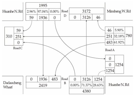
Figure 4.
Road traffic data from 8:00 a.m. to 9:00 a.m. on Huanhe N. Rd. and Minsheng W. Rd.
Figure 5 below shows the traffic flow and steering rate on Huanhe N. Rd. and Minsheng W. Rd. when people get off work. The total leaving traffic flow of road D is 1645 vehicles, including 1556 vehicles with a straight traffic flow (94.59%), 89 vehicles with a right-turn traffic flow (5.41%) and zero vehicles with a left-turn traffic flow (0%). The total coming traffic flow of road D is 2554 vehicles, including 2502 vehicles with a straight traffic flow from road B, and 52 vehicles with a right-turn traffic flow from road A. Similarly, Huanhe N. Rd. is not allowed to turn left because Road C is a one-way street. It is necessary to note that the traffic flow between going to work and getting off work at rush hours is different, and therefore the traffic light cycle configuration must also be different.
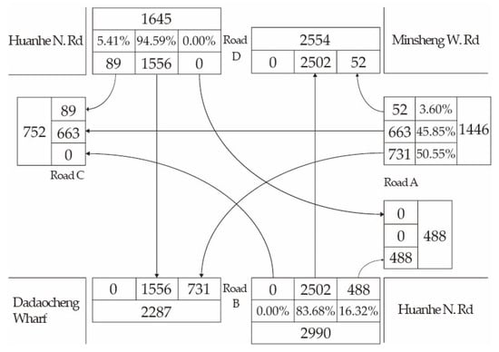
Figure 5.
Road traffic data from 5:00 p.m. to 6:00 p.m. on Huanhe N. Rd. and Minsheng W. Rd.
Figure 6 on the next page shows the intersection traffic data of Huanhe N. Rd and Nanjing W. Rd. As shown in Figure 6, From Road B to road D is a one-way street, so traffic flows can only flow to road D and road A. Road A’s traffic can only flow to road D. It can be seen from Figure 6 that the traffic volume of road B is much higher than that of the remaining intersections. This special intersection requires more cycle time for road B and road D.
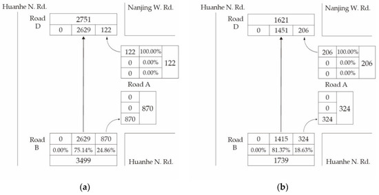
Figure 6.
Road traffic data of Huanhe N. Rd and Nanjing W. Rd. (a) 8:00 a.m. to 9:00 a.m. (b) 5:00 p.m. to 6:00 p.m.
Figure 7 and Figure 8 show the intersection traffic data of the Yanping N. Rd. and Minsheng W. Rd. when people go to work and get off work, respectively. Road B and road D are forbidden to turn left. Road C and road D have more traffic than the other two roads. If too much cycle time is given to road C and road D, they are able to handle more traffic. However, this will cause a significant idle state for both road A and road B. The key is to find a balanced traffic cycle configuration with our proposed mechanism adaptively.
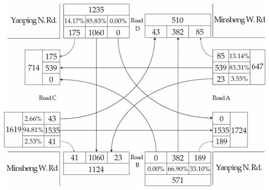
Figure 7.
Road traffic data from 8:00 a.m. to 9:00 a.m. on Minsheng W. Rd. and Yanping N. Rd.
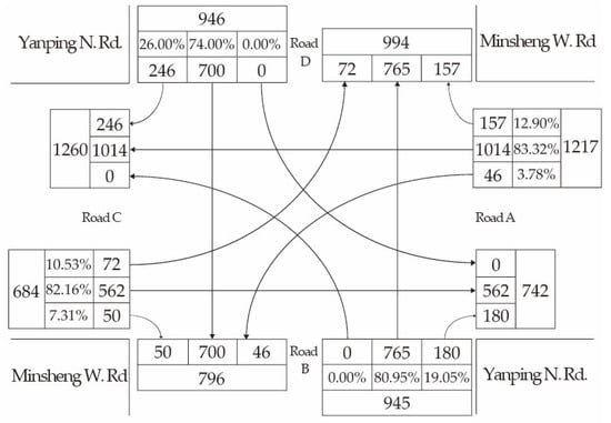
Figure 8.
Road traffic data from 5:00 p.m. to 6:00 p.m. on Minsheng W. Rd. and Yanping N. Rd.
3.2. Exhaustive Search Method
The Exhaustive search method, also known as brute-force search, is a general algorithm to solve problems. The Exhaustive search method enumerates all possible outcomes through the system, and then finds solutions to satisfy the conditions of the problem. Although the Exhaustive search method is easy to implement and to find the best solution, its computational cost is proportional to the number of solutions. As the complexity of the problem increases, the computational cost tends to grow very rapidly, and consequently a combinatorial explosion [35] occurs. According to the Taiwan Highway Capacity Manual [33], the traffic light cycle can be set from 30 s to 120 s, and each configuration cycle can be increased or decreased by 5 s. The exhaustive search method used in this experiment is to calculate all of the possible traffic light cycles in the interval, and find the best configuration cycle.
3.3. Q-Learning
Q-Learning [36] is a model free off policy reinforcement learning algorithm. The working principle is to update the expected value of the action in each state, and get a value for each possible state. Q-learning converges through repeated actions to achieve maximum expected return. This is indicated by updating the Q-value as below.
where Q is the expected value of the action At in the state St, St is the state of the vector t, At is the action of the vector t, R is the reward, α is the learning rate or step size and γ is the discount factor. Q-learning is able to learn the value of the action of all states. The cost of this algorithm is high, but it does get a good answer. The algorithm of the Q-learning approach is described in Algorithm 1.
| Algorithm 1. Q-learning. |
| Algorithm parameters: Step size , small |
| Initialize , for all , , arbitrarily except that (terminal, ·) = 0 |
| Loop for each episode: |
| Initialize S |
| Loop for each step of episode: |
| Choose from using policy derived from (e.g., -greedy) |
| Take action , observe , |
| until is terminal |
The ε-greedy algorithm [37] is one of the Multi-armed Bandit Algorithms. It can be divided into two parts: These are “explore” and “exploit.” “Explore” refers to the use of a random strategy to select the action to be performed. “Exploit” means using the original policy to select the action to be performed. In reinforcement learning, “explore” is often applied in the early stages of model training to help update more Q-values. “Exploit” is often used in the later stages of model training, where the information learned is enough, so you can follow the past experience. The ε-greedy action A that is used in Q-Learning is as follows.
3.4. Modified Q-Learning
The proposed modified Q-learning mechanism improves traditional Q-learning, and uses the Q-table to record the results of each learning. The total number of states is 19 × 19, which refers to the square of the total number of intervals from 30 s to 120 s with 5 s as one interval. The original traffic light cycle at the intersection is 60 s. There are four actions (action1, action2, action3 and action4) defined in this mechanism. Figure 9 shows the state transition diagram with four actions. The action1 is the North-South traffic light cycle plus five seconds, and the East-West traffic light cycle is fixed. The action2 is the North-South traffic light cycle minus five seconds, and the East-West traffic light cycle is fixed. The actioin3 is the East-West traffic light cycle plus five seconds, and the North-South traffic light cycle is fixed. The action4 is the East-West traffic light cycle minus five seconds, and the North-South traffic light cycle is fixed.
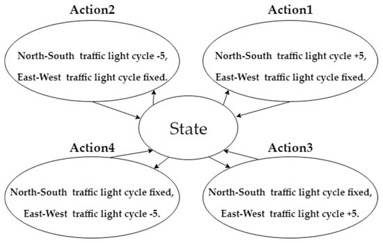
Figure 9.
State transition diagram with four actions.
The processing steps of the proposed modified Q-Learning mechanism are as follows:
- 1
- Initialize Q-table, new average vehicle delay time (New-AVDT) and best average vehicle delay time (Best-AVDT).
- 2
- While (Best-AVDT > New-AVDT):
- 2.1
- Starting the search from the current best state and randomly select the action of the maximum reward.
- 2.2
- Determining whether the selected action value is zero.
- 2.2.1
- If the action value is zero, then calculate whether New-AVDT is better than Best-AVDT before.
- 2.2.2
- If the New-AVDT is better than the Best-AVDT, update the best state and jump back to step (2); otherwise give a negative reward.
- 2.2.3
- If the action value is not zero, the agent randomly selects the new state and jumps to step (2.1).
- 2.3
- If the agent continues to find no better average vehicle delay time, the output is the best state.
- 3
- Agent recommends the best state cycle configuration.
The purpose of this experiment is to quickly find the minimum average vehicle delay time, so the selection action only looks at the current best state. If the action is not better than the previous average vehicle delay time (AVDT), it will give a negative reward (i.e., increase the AVDT), otherwise it will give a positive reward (i.e., decrease the AVDT). The reward function is listed in Equation (10). By using the Q-table to record the poor cycle configuration mode, the agent will not go to the poor state before the previous attempt, and then proceed to the better direction. However, such a method is prone to a local optimum. In order to solve this problem, this study adds a random state selection mechanism that effectively prevents the model from falling into a local optimum. The algorithm of the modified Q-learning approach is described in Algorithm 2, where Qbest represents the current small average delay time, and Sbest is the state of the current minimum average delay time.
| Algorithm 2. Modified Q-learning. |
| Algorithm parameters: Step size , small |
| let be the traffic light cycle time of the previous time period |
| let be the negative average delay time of the original traffic light cycle |
| Loop for each episode: |
| Initialize , for all , , arbitrarily, except that (terminal, ·) = |
| Loop for each step of episode: |
| Choose from using policy derived from (e.g., -greedy) |
| Take action , observe , |
| If then |
| until is terminal |
In Algorithm 2, the optimal Q value cannot be known before training, so the Qbest value must be updated by each training. Since the conventional Q-learning is a random initialization state, the Q value that causes the optimal state has a chance to be successively selected in the initial stage. Therefore, the Q value that causes the optimal state becomes too small, so the optimal state cannot be selected afterwards. In order to solve this problem, we modify the initial state by continuously updating Sbest, which ensures that the current state finds a better state in a shortest time. In this experiment, α is setting to 1, and γ is setting to 0; that is, only the current reward is considered. Because the purpose of this experiment is to quickly find the minimum average delay time, it is done by constantly updating the current rewards.
4. Experimental Result
This experiment collects the traffic flow, steering ratio, number of lanes and road types through a vehicle detector, and uses the data to find the approximately shortest vehicle delay time using our proposed mechanism. It is noted that the data set [30] is an open data provided by the Department of Transportation, Taipei City Government. The simulation tool is Taiwan Highway Capacity Software [31] that is developed by Taiwan Institute of Transportation. In order to evaluate the effectiveness of this mechanism, the exhaustive search method is used to find the configuration setting of the minimum average vehicle delay time.
Although the exhaustive search method may obtain the best solution, it will come with high computing costs. It means that the exhaustive search method will try all possible cases and then select the best solution. According to the Taiwan Highway Capacity Manual [33], the traffic light cycle can be adjusted from 30 s to 120 s, and each configuration cycle is increased or decreased by 5 s. The exhaustive search method used in this experiment is to calculate all the possible traffic light cycles in the interval and find the best configuration cycle. Because the experiment is the intersection of two Phases, the computational cost will increase rapidly as the number of phase increases, and consequently lead to excessive computing costs. Through the improved method proposed in this paper, the cycle of the traffic light is set to the state of modified Q-learning. Setting the four actions to increase or decrease the period for the optimized traffic cycle time, the proposed mechanism can save the time for the previous optimization and reduce the repeated search.
Figure 10, Figure 11 and Figure 12 show the results of vehicle delay by using the exhaustive search method for the three intersections, Huanhe N. Rd. and Minsheng W. Rd., Huanhe N. Rd and Nanjing W. Rd. and Yanping N. Rd. and Minsheng W. Rd., respectively. The x-axis, y-axis and z-axis represent the North-South traffic light cycle, East-West traffic light cycle and vehicle delay time, respectively. It is important to note that the traffic light cycle means the time of the green light. Figure 10 shows that the vehicle delay time distribution will vary greatly from time to time at the same intersection. The traffic flows in the morning and afternoon are different because the number of South-North (East-West) vehicles in the afternoon is much less (more) than the number of South-North vehicles in the morning (see Figure 4 and Figure 5). Figure 11 shows the distribution of vehicle delay time on the intersection of Huanhe N. Rd. and Nanjing W. Rd. The morning and afternoon delay times and traffic flows are similar because the South-North vehicle traffic rates are 75.14% and 81.37%, respectively (See Figure 6), and the number of the East-West vehicles is far less than the number of the South-North. Due to the high North-South vehicle traffic rate, the vehicle delay time increases and becomes significant when the traffic light (green light) time in the North-South intersection becomes smaller. Figure 12 shows the distribution of vehicle delay time on the intersection of Yanping N. Rd. and Minsheng W. Rd. The East-West traffic flow in the morning and afternoon is in the opposite direction (See Figure 7 and Figure 8). The vehicle delay time increases as the time of East-West (North-South) traffic light increases in the morning (in the afternoon).
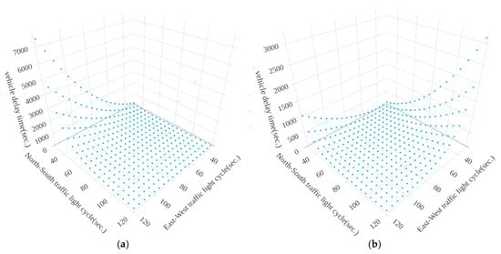
Figure 10.
The results of vehicle delay by using exhaustive search method on Huanhe N. Rd. and Minsheng W. Rd. (a) from 8:00 a.m. to 9:00 a.m. (b) from 5:00 p.m. to 6:00 p.m.
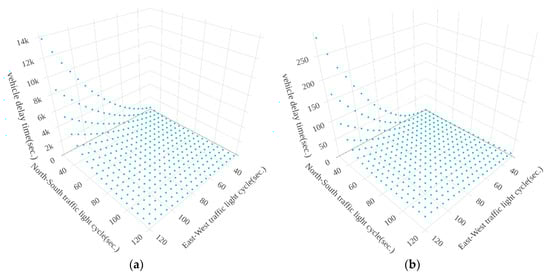
Figure 11.
The results of vehicle delay by using exhaustive search method on Huanhe N. Rd and Nanjing W. Rd. (a) from 8:00 a.m. to 9:00 a.m. (b) from 5:00 p.m. to 6:00 p.m.
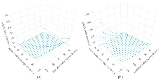
Figure 12.
The results of vehicle delay by using exhaustive search method on Yanping N. Rd. and Minsheng W. Rd. (a) from 8:00 a.m. to 9:00 a.m. (b) from 5:00 p.m. to 6:00 p.m.
Figure 13, Figure 14 and Figure 15 show the results of vehicle delay by using our proposed modified Q-learning mechanism for the three intersections: Huanhe N. Rd. and Minsheng W. Rd., Huanhe N. Rd and Nanjing W. Rd. and Yanping N. Rd. and Minsheng W. Rd., respectively. We actually conducted the experiments 30 times for our proposed modified Q-learning mechanism and averaged the results shown in Table 2, which will be discussed shortly. The contours shown in Figure 13, Figure 14 and Figure 15 just illustrate one experimental example for each case. Again, the x-axis, y-axis and z-axis represent the North-South traffic light cycle, East-West traffic light cycle and vehicle delay time (VDT), respectively. The start point is the initial state with x equal to 60 s and y equal to 60 s. The end point is the termination of the modified Q-learning. From the experimental results shown in Figure 13, the total number of steps for the modified Q-learning on Huanhe N. Rd and Nanjing W. Rd. from 8:00 a.m. to 9:00 a.m. is 24 steps with x, y and VDT equal to 35, 80 and 27, respectively. In addition, the total number of steps for the modified Q-learning on Huanhe N. Rd and Nanjing W. Rd. from 5:00 p.m. to 6:00 p.m. is 24 steps with x, y and VDT equal to 100, 70 and 68, respectively. Similarly, Figure 14 shows the experimental contours of the modified Q-learning vehicle delay on Huanhe N. Rd and Nanjing W. Rd. The corresponding total number of steps from 8:00 a.m. to 9:00 a.m. is 34 steps with x, y and VDT equal to 120, 30 and 31.3, respectively, and the corresponding total number of steps from 5:00 p.m. to 6:00 p.m. is 25 steps with x, y and VDT equal to 45, 30 and 6.9, respectively. Finally, Figure 15 illustrates the experimental contours of the modified Q-learning vehicle delay on Yanping N. Rd. and Minsheng W. Rd. The total number of steps from 8:00 a.m. to 9:00 a.m. is 25 steps with x, y and VDT equal to 30, 45 and 9.9, respectively. Along with this, the total number of steps from 5:00 p.m. to 6:00 p.m. is 24 steps with x, y and VDT equal to 30, 35 and 7.7, respectively.
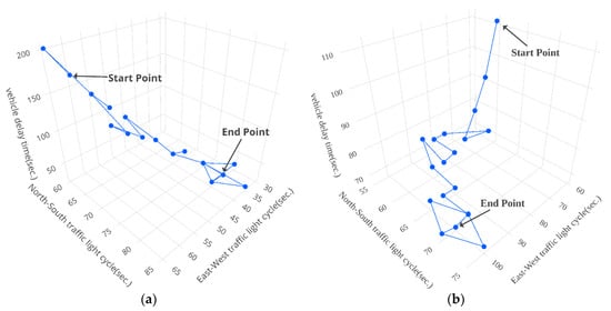
Figure 13.
The results of vehicle delay by using our proposed modified Q-learning mechanism on Huanhe N. Rd. and Minsheng W. Rd. (a) from 8:00 a.m. to 9:00 a.m. (b) from 5:00 p.m. to 6:00 p.m.
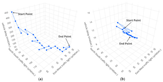
Figure 14.
The results of vehicle delay by using our proposed modified Q-learning mechanism on Huanhe N. Rd and Nanjing W. Rd. (a) from 8:00 a.m. to 9:00 a.m. (b) from 5:00 p.m. to 6:00 p.m.
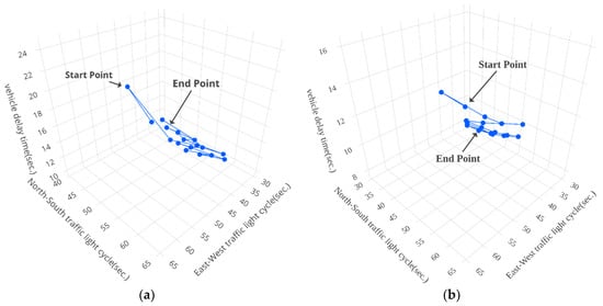
Figure 15.
The results of vehicle delay by using our proposed modified Q-learning mechanism on Yanping N. Rd. and Minsheng W. Rd. (a) from 8:00 a.m. to 9:00 a.m. (b) from 5:00 p.m. to 6:00 p.m.
Table 2.
The delay and processing steps for exhaustive search and modified Q-learning schemes.
Next, we conducted the experiments 30 times for our proposed modified Q-learning mechanism and averaged the results. The results of these experiments show that the number of processing steps of the proposed mechanism is under 34, and the error rate of the average vehicle delay time is within 9%. Table 2 shows a comparison of the results between modified Q-Learning and exhaustive search mechanisms. The proposed mechanism performs better than the exhaustive search scheme at the intersection of Yanping N. Rd. and Minsheng W. Rd. from 8:00 a.m. to 9:00 a.m., with a delay time error of 0% and an optimization rate of 12.67. For the results of the other two intersections, the average vehicle delay time of the proposed mechanism is still quite close to the exhaustive search scheme; however, the processing steps of the proposed mechanism were dropped by at least 9.91 times as compared to the exhaustive search scheme. It can be concluded that the proposed modified Q-learning mechanism can reduce the processing steps significantly, and in the meanwhile deliver a near-optimal average vehicle delay time. Therefore, the traffic light cycle configuration time of the proposed mechanism is capable of responding to the fast change of traffic peak time periods at the studied intersections.
The optimal traffic light cycle configuration time for each intersection is defined using the Exhaustive search scheme as calibration. Table 3 illustrates the error rate of the AVDT, defined in Equation (6). As can be seen from Table 3, if the difference between East-West and North-South light cycle times increases, the error rate E also increases. In this case, the proposed mechanism may just come out with local optimal results, and this occurrence produces around 8.9% of the error rate as compared to the optimal solution. On the contrary, if the difference between East-West and North-South light cycle times is insignificant, the error rate E is also small. In this case, the proposed model can find global optimal or approximate global optimal results.
Table 3.
The optimal cycle configuration time for each intersection.
Therefore, the proposed mechanism is capable of achieving good enough results with significantly fewer computational steps as compared to the Exhaustive search scheme.
5. Conclusions
In this paper, the exhaustive search scheme and the proposed modified Q-learning mechanism have been presented to find the optimal cycle configuration of traffic lights. The exhaustive search scheme can find the optimal results, but it must calculate all possible states, resulting in an increase in overall processing steps. On the contrary, the proposed modified Q-Learning mechanism has much fewer processing steps than the Exhaustive search scheme, while keeping the AVDT of the proposed mechanism very close to the results of the exhaustive search scheme. According to the simulation results, it shows that the proposed method can effectively reduce the AVDT under much fewer processing steps and can be applied to the needs of real case. It should be noted that the real traffic congestion will affect multiple intersections. Because of the high processing steps of multiple intersections, the exhaustive search method is unsuitable to be applied in the real traffic for searching the optimal solution.
However, in a well-developed city, it is not enough to solve the heavy traffic flow problem by just considering the traffic flows at a single intersection. This is because the traffic congestion at a single intersection will influence the traffic conditions of the surrounding intersections. Also the impact of the traffic congestion may vary with the distance between the congested intersection and the surrounding intersections. Therefore, in our future work, the traffic of k-nearby intersections will be taken into account, with different distances between surrounding intersections to reduce the AVDT. The static and dynamic training models will also be considered to solve the traffic congestion problems in the real traffic world.
Author Contributions
Software, Y.-X.L.; formal analysis, H.-C.C. and Y.-X.L.; investigation, H.-C.C., Y.-X.L. and L.-h.C.; data curation, Y.-X.L. and H.-C.C.; writing—original draft preparation, Y.-X.L., Y.-H.L., H.-C.C. and L.-h.C.; writing—review and editing, Y.-H.L., Y.-X.L. and H.-C.C.; visualization, H.-C.C., Y.-X.L. and L.-h.C.; supervision, H.-C.C.
Funding
This research was funded by Ministry of Science and Technology, Taiwan (MOST 107-2221-E-324-003-MY2).
Conflicts of Interest
The authors declare no conflict of interest.
References
- Sutton, R.S.; Barto, A.G. Reinforcement Learning: An Introduction, 2nd ed.; MIT Press: Cambridge, MA, USA, 2018; pp. 1–13. [Google Scholar]
- Wei, S.; Zou, Y.; Zhang, T.; Zhang, X.; Wang, W. Design and Experimental Validation of a Cooperative Adaptive Cruise Control System Based on Supervised Reinforcement Learning. Appl. Sci. 2018, 8, 1014. [Google Scholar] [CrossRef]
- Haarnoja, T.; Zhou, A.; Abbeel, P.; Levine, S. Soft actor-critic: Off-policy maximum entropy deep reinforcement learning with a stochastic actor. arXiv 2018, arXiv:1801.01290. [Google Scholar]
- Alsrehin, N.O.; Klaib, A.F.; Magableh, A. Intelligent Transportation and Control Systems Using Data Mining and Machine Learning Techniques: A Comprehensive Study. IEEE Access 2019, 7, 49830–49857. [Google Scholar] [CrossRef]
- Chen, J.; Li, D.; Zhang, G.; Zhang, X. Localized Space-Time Autoregressive Parameters Estimation for Traffic Flow Prediction in Urban Road Networks. Appl. Sci. 2018, 8, 277. [Google Scholar] [CrossRef]
- Qin, P.; Zhang, Y.; Wang, B.; Hu, Y. Grassmann Manifold Based State Analysis Method of Traffic Surveillance Video. Appl. Sci. 2019, 9, 1319. [Google Scholar] [CrossRef]
- Gupte, S.; Masoud, O.; Martin, R.F.; Papanikolopoulos, N.P. Detection and classification of vehicles. IEEE Trans. Intell. Transp. Syst. 2002, 3, 37–47. [Google Scholar] [CrossRef]
- Zaid, A.A.; Suhweil, Y.; Yaman, M.A. Smart controlling for traffic light time. In Proceedings of the IEEE Jordan Conference on Applied Electrical Engineering and Computing Technologies, Aqaba, Jordan, 11–13 October 2017. [Google Scholar]
- Nuss, D.; Thom, M.; Danzer, A.; Dietmayer, K. Fusion of laser and monocular camera data in object grid maps for vehicle environment perception. In Proceedings of the 17th International Conference on Information Fusion (FUSION), Salamanca, Spain, 7–10 July 2014. [Google Scholar]
- Silver, D.; Schrittwieser, J.; Simonyan, K.; Antonoglou, I.; Huang, A.; Guez, A.; Hubert, T.; Baker, L.; Lai, M.; Bolton, A.; et al. Mastering the game of go without human knowledge. Nature 2017, 550, 354–359. [Google Scholar] [CrossRef] [PubMed]
- Zhu, L.; Yu, F.R.; Wang, Y.; Ning, B. Big Data Analytics in Intelligent Transportation Systems: A Survey. IEEE Trans. Intell. Transp. Syst. 2019, 20, 383–398. [Google Scholar] [CrossRef]
- Qi, L.; Zhou, M.; Luan, W. Emergency Traffic-Light Control System Design for Intersections Subject to Accidents. IEEE Trans. Intell. Transp. Syst. 2016, 17, 170–183. [Google Scholar] [CrossRef]
- Chen, D. Research on traffic flow prediction in the big data environment based on the improved RBF neural network. IEEE Trans. Ind. Inform. 2017, 13, 2000–2008. [Google Scholar] [CrossRef]
- Li, H.; Wang, P.; Shen, C. Toward End-to-End Car License Plate Detection and Recognition with Deep Neural Networks. IEEE Trans. Intell. Transp. Syst. 2019, 20, 1126–1136. [Google Scholar] [CrossRef]
- Zhang, X.; Yu, L.; Wang, Y.; Xue, G.; Xu, Y. Intelligent travel and parking guidance system based on Internet of vehicle. In Proceedings of the IEEE 2nd Advanced Information Technology, Electronic and Automation Control Conference (IAEAC), Chongqing, China, 25–26 March 2017. [Google Scholar]
- Rekabdar, B.; Mousas, C. Dilated Convolutional Neural Network for Predicting Driver’s Activity. In Proceedings of the 21st International Conference on Intelligent Transportation Systems (ITSC), Maui, HI, USA, 4–7 November 2018. [Google Scholar]
- Singh, J. Experimental study for Gurmukhi Handwritten Character Recognition. In Proceedings of the 4th International Conference on Internet of Things: Smart Innovation and Usages (IoT-SIU), Ghaziabad, India, 18–19 April 2019. [Google Scholar]
- Krizhevsky, A.; Sutskever, I.; Hinton, G.E. Imagenet classification with deep convolutional neural networks. In Proceedings of the Neural Information Processing Systems (NIPS), Lake Tahoe, NV, USA, 3–8 December 2012. [Google Scholar]
- Mao, X.; Chang, S.; Shi, J.; Li, F.; Shi, R. Sentiment-Aware Word Embedding for Emotion Classification. Appl. Sci. 2019, 9, 1334. [Google Scholar] [CrossRef]
- Lucas, S.M. Game AI Research with Fast Planet Wars Variants. In Proceedings of the IEEE Conference on Computational Intelligence and Games (CIG), Maastricht, The Netherlands, 14–17 August 2018. [Google Scholar]
- Angarita-Zapata, J.S.; Masegosa, A.D.; Triguero, I. A Taxonomy of Traffic Forecasting Regression Problems from a Supervised Learning Perspective. IEEE Access 2019, 7, 68185–68205. [Google Scholar] [CrossRef]
- Dike, H.U.; Zhou, Y.; Deveerasetty, K.K.; Wu, Q. Unsupervised Learning Based On Artificial Neural Network: A Review. In Proceedings of the IEEE International Conference on Cyborg and Bionic Systems (CBS), Shenzhen, China, 25–27 October 2018. [Google Scholar]
- Kochenderfer, M.J.; Monath, N. Compression of Optimal Value Functions for Markov Decision Processes. In Proceedings of the Data Compression Conference, Snowbird, UT, USA, 20–22 March 2013. [Google Scholar]
- Sun, C. Fundamental Q-learning Algorithm in Finding Optimal Policy. In Proceedings of the International Conference on Smart Grid and Electrical Automation (ICSGEA), Changsha, China, 27–28 May 2017. [Google Scholar]
- Schilperoort, J.; Mak, I.; Drugan, M.M.; Wiering, M.A. Learning to Play Pac-Xon with Q-Learning and Two Double Q-Learning Variants. In Proceedings of the IEEE Symposium Series on Computational Intelligence (SSCI), Bangalore, India, 18–21 November 2018. [Google Scholar]
- Lu, K.; Xu, J.M.; Li, Y.S. An optimization method for single intersection’s signal timing based on SARSA(λ) algorithm. In Proceedings of the Chinese Control and Decision Conference, Yantai, China, 2–4 July 2008. [Google Scholar]
- Cheng, Q.; Wang, X.; Yang, J.; Shen, L. Automated Enemy Avoidance of Unmanned Aerial Vehicles Based on Reinforcement Learning. Appl. Sci. 2019, 9, 669. [Google Scholar] [CrossRef]
- Cao, X.R. A basic formula for online policy gradient algorithms. IEEE Trans. Autom. Control. 2005, 50, 696–699. [Google Scholar]
- Sehnke, F.; Osendorfer, C.; Rückstieß, T.; Gravesa, A.; Peters, J.; Schmidhuber, J. Parameter-exploring Policy Gradients. J. Neural Netw. 2010, 23, 511–559. [Google Scholar] [CrossRef] [PubMed]
- Taipei City Government Department of Transportation. Available online: https://www.dot.gov.taipei/ (accessed on 30 July 2019).
- Taiwan Highway Capacity Software. Available online: https://thcs.iot.gov.tw/WebForm2.aspx (accessed on 26 October 2019).
- Vukmirović, S.; Čapko, Z.; Babić, A. The Exhaustive Search Algorithm in the Transport network optimization on the example of Urban Agglomeration Rijeka. In Proceedings of the International Convention on Information and Communication Technology, Electronics and Microelectronics (MIPRO), Opatija, Croatia, 20–24 May 2019. [Google Scholar]
- Taiwan Road Capacity Manual. Available online: https://thcs.iot.gov.tw/WebForm3.aspx (accessed on 26 October 2019).
- Road Traffic Sign Marking Line Setting Plan. Available online: https://law.moj.gov.tw/LawClass/LawAll.aspx?pcode=K0040014 (accessed on 26 October 2019).
- Combinatorial Explosion. Available online: http://pespmc1.vub.ac.be/ASC/COMBIN_EXPLO.html (accessed on 30 July 2019).
- Luo, B.; Liu, D.; Huang, T.; Wang, D. Model-Free Optimal Tracking Control via Critic-Only Q-Learning. IEEE Trans. Neural Netw. Learn. Syst. 2016, 27, 2134–2144. [Google Scholar] [CrossRef] [PubMed]
- Katoh, M.; Shimotani, R.; Tokushige, K. Integrated Multiagent Course Search to Goal by Epsilon-Greedy Learning Strategy: Dual-Probability Approximation Searching. In Proceedings of the IEEE International Conference on Systems, Man, and Cybernetics, Kowloon, China, 9–12 October 2015. [Google Scholar]


© 2019 by the authors. Licensee MDPI, Basel, Switzerland. This article is an open access article distributed under the terms and conditions of the Creative Commons Attribution (CC BY) license (http://creativecommons.org/licenses/by/4.0/).