A New Adaptive Fuzzy PID Controller Based on Riccati-Like Equation with Application to Vibration Control of Vehicle Seat Suspension

Abstract

A new controller based on the modified Riccati-like Equation is developed in this paper. The interval type 2 fuzzy model is applied and embedded in the controller to ensure the robustness to parameter uncertainties and also to support calculation progress. The proposed input control includes equivalent control and robustness control. The equivalent control is found from the conventional analysis with the sliding surface, but this control is not sufficient to resolve the uncertainties and disturbances such as error approximation of the fuzzy model. Thus, a proportional-integral-derivative (PID) controller and matrices of the traditional model of Riccati equation are utilized to ensure the robustness. In the synthesis of this control part, the H infinity technique is adopted and the stability of the system is proved using Lyapunov stability. Subsequently, to validate the effectiveness of the proposed controller, it was applied to vibration control of a vehicle seat suspension with a magnetorheological (MR) damper subjected to stiffness variation due to the magnitude of the input current. In this problem, two types of road conditions, bump and random step wave, were adopted and control performance was evaluated in both simulations and experiments. Based on these evaluations, the proposed controller provides high control performances, effectively controlling the acceleration and displacement at the driver position.

1. Introduction

The more modern is the machine used, the more complicated is the control required. This slogan is currently popular in various industrial societies. The objectives of this slogan, of course, are to achieve higher control efficiency, less power consumption, higher safety and so forth. In control of complicated systems, the model of adaptive control is one of the favored solutions because of its stability and high efficiency. There are two types of adaptive control: indirect and direct controls. The indirect model is the best choice for design of adaptive control, which can be changed to direct model by applying constant parameters for the denominator in main input control. In addition, the main advantage of the adaptive control is its combination with other controls such as fuzzy model, PID (Proportional-Integral-Derivative), optimal control, and sliding mode control. In [1], the indirect adaptive model was studied for MIMO (Multiple-Input and Multiple-Output) nonlinear system. In this study, three main factors of the control, namely actuator fault, unknown system function, and sensor fault, were considered and the fuzzy model was applied in the adaptation laws related to the above three factors. The controller developed in [2] is different from the controller in [1], using a new function as a reset mechanism for the adaptive control law. The objective of the reset solution was to improve the transient performance by leading the estimated parameters to the best values at the initial steps of adaptation. In fact, the reset mechanism was designed by setting a time related boundary of stability and instability times, and this boundary was solved by adaptation laws. Recently, the adaptive control has been used for control unknown phenomena such as dead-zone [3]. Basically, the unknown problem in control was solved by using Nussbaum-type function, and the parameter of the Nussbaum function was updated by adaptation law and the fuzzy model. From the above three studies on adaptive control, the Lyapunov and its modification are main functions to evaluate the stability and design of adaptation laws. The technique using PID in adaptive control [4,5,6,7,8,9,10] was also continuously analyzed.

The sliding surface of sliding mode control was used as a first solid function for design of adaptive control and the PID control was used to ensure control robustness through adaptation laws [4]. It is noted that the technique in [4] followed the conventional design of adaptive control with non-modification of the robustness control to improve performance of the system. Several works similar to the one in [4] have been undertaken [5,6,7]. The technique proposed in [8] was basically similar to the work done in [4,5,6,7], where the main input control (robust control) used an additive input uncertainty and regression function. Thus, the adaptation laws were derived from the matrices of the conventional Lyapunov equation and error vector. The disadvantage of this approach is less flexibility with the change of disturbances of environment, although the uncertainty of system can be controlled well. The flexible property of the adaptation laws with the Lyapunov equation through Riccati-like equation with PID was studied in [9]. This study presented a new combination of the Riccati-like equation with the conventional robustness PID control, in which the sliding surface is the main parameter of the adaptation laws. Another solution is to use exponential function as presented in [10] where the library of design PID control in adaptive control can be formulated. The application of the modified Riccati-like equation was also studied in [11,12,13,14]. These studies demonstrated that the Lyapunov equation through the Riccati-like equation could improve control performance of the system subjected to uncertainties and/or disturbances. It is noted that other effective methods for calculation based on smart grid controller associated with the energy management have been developed in [15,16,17]. In these methods, the global optimization of points related to the mesh of controlled sub-station is used to achieve control robustness.

The main technical contribution of this work is to develop a new controller which is robust to uncertainties and disturbances. Especially, in this work, the model of interval type 2 fuzzy (IT2FNN) is used, which has several salient features [18,19,20,21]. Then, to achieve fast calculation of the IT2FNN, the granular clustering method [18] is used. The application of the IT2FNN can ensure enhanced control performances in the presence of disturbances and uncertainties of the system by optimizing the values for calculation of the embedded functions. To achieve the final goal of this work, the following are sequentially undertaken: (i) a new hybrid control including sliding mode control, H infinity technique, PID, and fuzzy neural network model is formulated; (ii) a new Riccati-like equation with the parameters of sliding surface of sliding mode control, PID, and fuzzified value is proposed; and (iii) the proposed control is applied to vibration control of the vehicle seat suspension system equipped with MR damper. The proposed controller is evaluated through both computer simulation and experimental realization, and the control effectiveness is validated showing well-controlled acceleration and displacement at the driver position.

2. New Adaptive Fuzzy PID Controller

2.1. Interval Type 2 Fuzzy Neural Network Model

The model of interval type 2 fuzzy (IT2FNN) and the granular clustering method in [18,21] are adopted to design a robust controller. The rule base of IT2FNN can be expressed as follows.

$$R_{nf}{}^j:\mathbf{If}{h}_{n1}\mathrm{is}{H}_{nf1}^j\mathrm{and}\dots \mathrm{and}{h}_{nm}\mathrm{is}{H}_{nfm}^j\mathbf{Then}g\mathrm{is}{a}_0^j+{\displaystyle \sum _{i=1}^m{a}_i^j}{h}_{ni}$$

(1)

where $H_{nfi}^j\left(i=1,\dots ,m;j=1,\dots ,n\right)$ are the fuzzy sets of the data, $n$ is the number of fuzzy rules, and $a_i^j$ are the interval sets of the fuzzy model. The output of the fuzzy model [20,21] is then determined by

$$g_{nf}=\frac{g_{nl}+g_{nr}}{2}=\frac{{\mathsf{\theta }}_{nl}^T{\mathsf{\xi }}_{nl}^f+{\mathsf{\theta }}_{nr}^T{\mathsf{\xi }}_{nr}^f}{2}$$

(2)

In the above, ${\mathsf{\theta }}_{nl}^T=\left[w_1^l{w}_2^l{w}_3^l\dots w_m^l\right]$ and ${\mathsf{\theta }}_{nr}^T=\left[w_1^r{w}_2^r{w}_3^r\dots w_m^r\right]$ are the weighting vectors, and the weighted firing strength vectors are given by ${\mathsf{\xi }}_{nl}^f$ and ${\mathsf{\xi }}_{nr}^f$.

2.2. Adaptive Fuzzy PID Control

In this study, a general form of the mth-order nonlinear system is used as follows:

$${\dot{x}}_{ns}=f_n\left(x_{ns}\right)+g_n\left(x_{ns}\right)u\left(t\right)+d_n\left(t\right)$$

(3)

In Equation (3), the functions $f_n\left(x_{ns}\right)\in R^m$ and $g_n\left(x_{ns}\right)\in R^m$ are two unknown vectors; $u\left(t\right)\in R^1$ is the input control; $d_n\left(t\right)\in R^m$ is the disturbance (internal and external disturbances); and $\left|d_n\left(t\right)\right|\le \delta d_n$, where $\delta d_n\in R^m$ is boundary of $d_n\left(t\right)$ and $x_{ns}=\left[x_{n1}{,x}_{n2},\dots {,x}_{nm}\right]={[x_{n1},{\dot{x}}_{n1},\dots {,x}_{n1}{}^{(m-1)}]}^T\in R^m$ is the state variables. The system in Equation (3) can be rewritten as follows.

$${\dot{x}}_{ns}=f_{n0}(x_{ns})+g_{n0}(x_{ns})u\left(t\right)+D_n\left(t\right)$$

(4)

where $D_n\left(t\right)=\delta f_n+\delta g_{n}u\left(t\right)+d_n(t)$ denotes the disturbances given by

$$\begin{gathered} D_n={\left[0,0,\dots ,D_{n0}\right]}^T,f_{n0}\left(x_{ns}\right)={\left[x_{n2},\dots ,x_{nm},f_{n0}\right]}^T,g_{n0}\left(x_{ns}\right)={\left[0,\dots ,0,g_{n0}\right]}^T, \\ \mathsf{\delta }{f}_n={\left[0,0,\dots ,\delta f_{n0}\right]}^T,\mathsf{\delta }{g}_n={\left[0,0,\dots ,\delta g_{n0}\right]}^T \end{gathered}$$

Based on Equation (2), the relationship between the system in Equation (4) and IT2FNN is determined as follows:

$$f_{n00}\left(x_{ns}\right)=f_{n0}\left(x_{ns}\right)g_f={\mathsf{\theta }}_{nf}{\mathsf{\xi }}_{nf}$$

(5)

$$g_{n00}\left(x_{ns}\right)=g_{n0}\left(x_{ns}\right)g_{nf}={\mathsf{\theta }}_{ng}{\mathsf{\xi }}_{ng}$$

(6)

where ${\mathsf{\theta }}_{nf}={\left[{\mathsf{\theta }}_{nf}^l,{\mathsf{\theta }}_{nf}^u\right]}^T$, ${\mathsf{\theta }}_g={\left[{\mathsf{\theta }}_g^l,{\mathsf{\theta }}_g^u\right]}^T$ and ${\mathsf{\xi }}_{nf}={\mathsf{\xi }}_{ng}=\left[{\mathsf{\xi }}_{nl},{\mathsf{\xi }}_{nu}\right]$. Note that ${\mathsf{\theta }}_{nf},{\mathsf{\theta }}_{ng}$ are the centroid of consequent vectors. ${\mathsf{\xi }}_{nf}$ and ${\mathsf{\xi }}_{ng}$ are consequent membership vectors of $f_n,g_n$, respectively. The sliding surface $s_{\Delta }$ of sliding mode control is defined as follows.

$$s_{\Delta }=k_1{x}_{n1}+k_2{x}_{n2}+k_3{x}_{n3}+\dots +k_m{x}_m={\displaystyle \sum _{i=1}^m{k}_i{x}_i}$$

(7)

where $K_m=\left[k_m,k_{m-1},k_{m-2},\dots ,k_1\right]$. It is noted that $k_m=1$ in this analysis. The sliding surface in Equation (7) is rewritten as follows:

$$x_{nm}=-k_1{x}_{n1}-k_2{x}_{n2}-k_3{x}_{n3}-\dots -k_{m-1}{x}_{nm-1}+s_{\Delta }$$

(8)

A new vector ${\tilde{x}}_s$ is defined by ${\tilde{x}}_{ns}={\left[x_{n1}{x}_{n2}{x}_{n3}\dots x_{nm-1}\right]}^T$, and thus the system in Equation (4) is rewritten as:

$${\dot{\tilde{x}}}_{ns}=S_{n1}{\tilde{x}}_{ns}+S_{n2}^T{s}_{\Delta }$$

(9)

where

$$S_{n1}=\left[\begin{array}{cccc}0& 1& 0& \begin{array}{cc}\dots & 0\end{array}\\ 0& 0& 1& \begin{array}{cc}\dots & 0\end{array}\\ .& .& .& \begin{array}{cc}\dots & .\end{array}\\ -k_1& -k_2& -k_3& \begin{array}{cc}\dots & -k_{m-1}\end{array}\end{array}\right],S_{n2}=\left[\begin{array}{c}0\\ 0\\ .\\ 1\end{array}\right]$$

The derivative of Equation (7) is obtained as follows.

$${\dot{s}}_{\Delta }=k_1{\dot{x}}_{n1}+k_2{\dot{x}}_{n2}+k_3{\dot{x}}_{n3}+\dots +k_{m-1}{\dot{x}}_{nm-1}+f_{n0}(x_{ns})+g_{n0}(x_{ns})u\left(t\right)+D_n\left(t\right)$$

(10)

The lumped uncertainty is expressed by

$$w_{nl}={\tilde{\gamma }}_{nf}{\xi }_{nf}+{\tilde{\gamma }}_{ng}{\xi }_{ng}u+D_n$$

(11)

where ${\tilde{\gamma }}_{nf}=f_{n0}\left(x_{ns}\right)-f_{n00}^{\ast }\left(x_{ns}\right)$ and ${\tilde{\gamma }}_{ng}=g_{n0}\left(x_{ns}\right)-g_{n00}^{\ast }\left(x_{ns}\right)$. Substituting Equation (11) into Equation (10) yields the following equation.

$${\dot{s}}_{\Delta }={\displaystyle \sum _{i=1}^{m-1}{k}_i{x}_{ni+1}}+f_{n00}^{\ast }\left(x_{ns}\right)+g_{n00}^{\ast }\left(x_{ns}\right)u+w_{nl}$$

(12)

Then, Equation (12) can be written by substituting values of the fuzzy mode as

$${\dot{s}}_{\Delta }={\displaystyle \sum _{i=1}^{m-1}{k}_i{x}_{ni+1}}+{\theta }_{nf}^{\ast }{\xi }_{nf}+{\theta }_{ng}^{\ast }{\xi }_{ng}u+w_{nl}$$

(13)

where

$$\begin{gathered} {\theta }_{nf}^{\ast }=\arg {\min }_{{\theta }_{nf}\in \Delta {\theta }_{nf}}\left[{\sup }_{x_{ns}\in \Delta x_n}\left|f_n\left(x_{ns}\right)-f_{n00}^{}\left(x_{ns}\right)\right|\right], \\ {\theta }_{ng}^{\ast }=\arg {\min }_{{\theta }_{ng}\in \Delta {\theta }_{ng}}\left[{\sup }_{x_{ns}\in \Delta x_n}\left|g_n\left(x_{ns}\right)-g_{n00}^{}\left(x_{ns}\right)\right|\right],\Delta {\theta }_{nf}=\left\{{\theta }_{nf}\in R^m,\Vert {\theta }_{nf}\Vert \le {\epsilon }_{nf}\right\}, \\ \Delta {\theta }_{ng}=\left\{{\theta }_{ng}\in R^m,\Vert {\theta }_{ng}\Vert \le {\epsilon }_{ng}\right\},\Delta x_n=\left\{x_{ns}\in R^m,\Vert x_{ns}\Vert \le {\epsilon }_{nx}\right\} \end{gathered}$$

In the above equations, ${\epsilon }_{nf},{\epsilon }_{ng},{\epsilon }_{nx}$ are constant boundaries. An equivalent control of the system is derived from Equation (13) based on assumption of $w_{nl}\approx 0$:

$$u_{n1}=-\frac{1}{{\widehat{\theta }}_{ng}{\xi }_{ng}}\left({\displaystyle \sum _{i=1}^{m-1}{k}_i{x}_{ni+1}}+{\widehat{\theta }}_{nf}{\xi }_{nf}\right)$$

(14)

To guarantee the robustness and stability in control, a new robust control $u_{n2}$ is suggested as follows:

$$u_{n2}=\frac{1}{{\widehat{\theta }}_{ng}{\xi }_{ng}}\left(\begin{array}{l}-{\displaystyle \sum _{i=1}^{m-1}{P}_{\left(m-1\right)i}{x}_{ni}}-\frac{s_{\Delta }}{\beta }+\frac{1}{2}{\Gamma }_n{s}_{\Delta }{\xi }_{fz}{\tilde{x}}_{ns}{P}_n{S}_{n2}{S}_{n2}^T{P}_n{\tilde{x}}_{ns}{}^T+K_P{S}_2^T{E}_n{E}_n^T{P}_n{B}_P+\\ +K_I{\displaystyle \int S_2^T{E}_n{E}_n^T{P}_n{B}_{P}dt+K_D{S}_2^T{\dot{E}}_n{\dot{E}}_n^T{P}_n{B}_P}\end{array}\right)$$

(15)

where $e_n=x_{nd}-x_{ns},E_n=[{\mathrm{e}}_{\mathrm{n}1}{,\mathrm{e}}_{\mathrm{n}2},\mathrm{\dots }{,\mathrm{e}}_{\mathrm{nm}}]$ is tracking error and $x_d$ is the desired value. The value of $B_P$ is determined as follows:

$${\dot{x}}_{ns}=f_{n0}(x_{ns})+g_{n0}(x_{ns})u\left(t\right)+D_n\left(t\right)=A_P\left(x_{ns}\left(t\right),t\right)x_{ns}\left(t\right)+B_P\left(x_{ns}\left(t\right),t\right)u\left(t\right)+D_n\left(t\right)$$

(16)

where $A_P\in R^{m\times m},B_P\in R^{m\times v},u\left(t\right)\in R^v\left(v=1\right)$. The value ${\Gamma }_n$ is the adaptive parameter related the modified Riccati-like equation, and its boundary is given by $\Delta {\Gamma }_n=\left\{{\Gamma }_n\in R,\Vert {\Gamma }_n\Vert \le {\epsilon }_{n\Gamma },{\Gamma }_n{\xi }_{fz}\le \rho \right\}$; ${\epsilon }_{n\Gamma }$ is constant boundary. The matrix $P_n=P_n^T\ge 0$ in which its result is a solution of a new modified Riccati-like equation given by

$$\begin{array}{l}{P}_n{S}_{n1}+S_{n1}^T{P}_n+Q_n-s_{\Delta }{\Gamma }_n{\xi }_{fz}{P}_n{S}_{n2}{S}_{n2}^T{P}_n+\rho P_n{S}_{n2}{S}_{n2}^{T}P-K_P{\xi }_{fz}{S}_{n2}^T{E}_n{E}_n^T{P}_n{B}_P-\\ -K_I{\xi }_{fz}{\displaystyle \int S_{n2}^T{E}_n{E}_n^T{P}_n{B}_{P}dt-K_D{\xi }_{fz}{S}_{n2}^T{\dot{E}}_n{\dot{E}}_n^T{P}_n{B}_P}=0\end{array}$$

(17)

where $\left\{s_{\Delta }{\Gamma }_n{\xi }_{fz},K_P{\xi }_{fz},K_I{\xi }_{fz},K_D{\xi }_{fz}\right\}\le \rho$. The boundaries of $K_P$, $K_I$, and $K_D$ are determined as $\Delta K_P=\left\{K_P\in R,\Vert K_P\Vert \le {\epsilon }_{nKP}\right\}$, $\Delta K_I=\left\{K_I\in R,\Vert K_I\Vert \le {\epsilon }_{nKI}\right\}$, and $\Delta K_D=\left\{K_D\in R,\Vert K_D\Vert \le {\epsilon }_{nKD}\right\}$, respectively. In these boundaries, ${\epsilon }_{nKP}$, ${\epsilon }_{nKI}$ and ${\epsilon }_{nKD}$ are positive constants. Finally, the control $u$ of the system is determined as follows.

$$u=u_{n1}+u_{n2}$$

(18)

Remark 1.

The modified Riccati-like equation given in Equation (17) is a new format including three parameters of the classical PID control and the fuzzy neural networks model. This format opens a new approach to improve performance of the system through the adaptation laws. The conventional Riccati-like equation is fixed with elements related to the Hamiltonian equation, matrices and vectors of the system. The expansion of the Riccati-like equation proposed in this work can bring a flexibility for calculation and combination with other controllers to enhance control robustness against severe disturbances.

Remark 2.

To evaluate the stability and robustness of the system, Lyapunov function of the system in Equation (3) is suggested as follows.

$$V=\frac{1}{2}{s}_{\Delta }{}^2+\frac{1}{2}{\tilde{x}}_{ns}{P}_n{\tilde{x}}_{ns}{}^T+\frac{1}{2{\eta }_1}{\tilde{\gamma }}_{nf}^2+\frac{1}{2{\eta }_2}{\tilde{\gamma }}_{ng}^2+\frac{1}{2{\eta }_3}{\Gamma }_n^2+\frac{1}{2{\eta }_4}{K}_P^2+\frac{1}{2{\eta }_5}{K}_I^2+\frac{1}{2{\eta }_6}{K}_D^2$$

(19)

Based on the evaluation of the Lyapunov equation, six adaptation laws are found:

$${\dot{\tilde{\gamma }}}_{nf}=-{\eta }_1{s}_{\Delta }{\xi }_{nf}$$

(20)

$${\dot{\tilde{\gamma }}}_{ng}=-{\eta }_2{s}_{\Delta }{\xi }_{ng}u$$

(21)

$${\dot{\Gamma }}_n=-{\eta }_3{s}_{\Delta }{\xi }_{fz}{\tilde{x}}_{ns}{P}_n{S}_{n2}{S}_{n2}^T{P}_n{\tilde{x}}_{ns}{}^T$$

(22)

$${\dot{K}}_P=-{\eta }_4\left(s_{\Delta }{S}_{n2}^T{E}_n{E}_n^T{P}_n{B}_P+\frac{1}{2}{\xi }_{fz}{\tilde{x}}_{ns}{S}_{n2}^T{E}_n{E}_n^T{P}_n{B}_P{\tilde{x}}_{ns}{}^T\right)$$

(23)

$${\dot{K}}_I=-{\eta }_5\left(s_{\Delta }{\displaystyle \int S_{n2}^T{E}_n{E}_n^T{P}_n{B}_P}dt+\frac{1}{2}{\xi }_{fz}{\tilde{x}}_{ns}\left[{\displaystyle \int S_{n2}^T{E}_n{E}_n^T{P}_n{B}_P}dt\right]{\tilde{x}}_{ns}{}^T\right)$$

(24)

$${\dot{K}}_D=-{\eta }_6\left(s_{\Delta }{S}_{n2}^T{\dot{E}}_n{\dot{E}}_n^T{P}_n{B}_P+\frac{1}{2}{\xi }_{fz}{\tilde{x}}_{ns}\left[S_{n2}^{}{S}_{n2}^T{\dot{E}}_n{\dot{E}}_n^T{P}_n{B}_P\right]{\tilde{x}}_{ns}{}^T\right)$$

(25)

Theorem 1.

The main adaptation laws of the proposed adaptive PID controller given by Equations (20)–(25) are modified to satisfy Lyapunov stability using the projection algorithm as follows.

$${\dot{\tilde{\gamma }}}_{nf}=\{\begin{array}{c}\begin{array}{cc}-{\eta }_1{s}_{\Delta }{\xi }_{nf}& if\Vert {\tilde{\gamma }}_{\mathrm{nf}}\Vert <{\epsilon }_{nf}or\left(\Vert {\tilde{\gamma }}_{nf}\Vert ={\epsilon }_{nf}and{s}_{\Delta }{\xi }_{nf}{\tilde{\gamma }}_{nf}\ge 0\right)\end{array}\\ \begin{array}{cc}-{\eta }_1{s}_{\Delta }{\xi }_{nf}+{\eta }_1\frac{\left({\Vert {\tilde{\gamma }}_{nf}\Vert }^2-{\epsilon }_{nf}\right)s_{\Delta }{\xi }_{nf}{\tilde{\gamma }}_{nf}}{{\delta }_1{\Vert {\tilde{\gamma }}_{nf}\Vert }^2}& if\Vert {\tilde{\gamma }}_{nf}\Vert ={\epsilon }_{nf}and{s}_{\Delta }{\xi }_{nf}{\tilde{\gamma }}_{nf}<0\end{array}\end{array}$$

(26)

$${\dot{\tilde{\gamma }}}_{ng}=\{\begin{array}{c}\begin{array}{cc}-{\eta }_2{s}_{\Delta }{\xi }_{ng}u& if\Vert {\tilde{\gamma }}_{\mathrm{ng}}\Vert <{\epsilon }_{ng}or\left(\Vert {\tilde{\gamma }}_{\mathrm{g}}\Vert ={\epsilon }_{ng}and{s}_{\Delta }{\xi }_{ng}u{\tilde{\gamma }}_{\mathrm{ng}}\ge 0\right)\end{array}\\ \begin{array}{cc}-{\eta }_2{s}_{\Delta }{\xi }_{ng}u+{\eta }_2\frac{\left({\Vert {\tilde{\gamma }}_{ng}\Vert }^2-{\epsilon }_{ng}\right)s_{\Delta }{\xi }_{ng}u{\tilde{\gamma }}_{ng}}{{\delta }_2{\Vert {\tilde{\gamma }}_{ng}\Vert }^2}& if\Vert {\tilde{\gamma }}_{\mathrm{ng}}\Vert ={\epsilon }_{ng}and{s}_{\Delta }{\xi }_{ng}u{\tilde{\gamma }}_{\mathrm{ng}}<0\end{array}\end{array}$$

(27)

$${\dot{\Gamma }}_n=\{\begin{array}{c}\begin{array}{cc}-{\eta }_3{s}_{\Delta }{\xi }_{fz}{\tilde{x}}_{ns}{P}_n{S}_{n2}{S}_{n2}^T{P}_n{\tilde{x}}_{ns}{}^T& if\Vert {\Gamma }_n\Vert <{\epsilon }_{n\Gamma }or\left(\Vert {\Gamma }_n\Vert ={\epsilon }_{n\Gamma }+{\delta }_{\text{3}}and{s}_{\Delta }{\xi }_{fz}{\tilde{x}}_{ns}{P}_n{S}_{n2}{S}_{n2}^T{P}_n{\tilde{x}}_{ns}{}^T{\Gamma }_n\ge \text{0}\right)\end{array}\\ \begin{array}{cc}-{\eta }_3{s}_{\Delta }{\xi }_{fz}{\tilde{x}}_{ns}{P}_n{S}_{n2}{S}_{n2}^T{P}_n{\tilde{x}}_{ns}{}^T+{\eta }_3\frac{\left({\Vert {\Gamma }_n\Vert }^2-{\epsilon }_{n\Gamma }\right)s_{\Delta }{\xi }_{fz}{\tilde{x}}_{ns}{P}_n{S}_{n2}{S}_{n2}^T{P}_n{\tilde{x}}_{ns}{}^T{\Gamma }_n}{{\delta }_3{\Vert {\Gamma }_n\Vert }^2}& \begin{array}{l}if\Vert {\Gamma }_n\Vert ={\epsilon }_{n\Gamma }and\\ s_{\Delta }{\xi }_{fz}{\tilde{x}}_{ns}{P}_n{S}_{n2}{S}_{n2}^T{P}_n{\tilde{x}}_{ns}{}^T{\Gamma }_n<0\end{array}\end{array}\end{array}$$

(28)

$${\dot{K}}_P=\{\begin{array}{c}\begin{array}{cc}-{\eta }_4\left(\begin{array}{l}{s}_{\Delta }{S}_{n2}^T{E}_n{E}_n^T{P}_n{B}_P+\\ +\frac{1}{2}{\xi }_{fz}{\tilde{x}}_{ns}{S}_{n2}^T{E}_n{E}_n^T{P}_n{B}_P{\tilde{x}}_{ns}{}^T\end{array}\right)& \begin{array}{l}if\Vert K_P\Vert <{\epsilon }_{nKP}or\\ \left(\begin{array}{l}\Vert K_P\Vert ={\epsilon }_{nKP}\\ and\left(\begin{array}{l}{s}_{\Delta }{S}_{n2}^T{E}_n{E}_n^T{P}_n{B}_P+\\ +\frac{1}{2}{\xi }_{fz}{\tilde{x}}_{ns}{S}_{n2}^T{E}_n{E}_n^T{P}_n{B}_P{\tilde{x}}_{ns}{}^T\end{array}\right)K_P\ge \text{0}\end{array}\right)\end{array}\end{array}\\ \begin{array}{cc}\begin{array}{l}-{\eta }_4\left(\begin{array}{l}{s}_{\Delta }{S}_{n2}^T{E}_n{E}_n^T{P}_n{B}_P+\\ +\frac{1}{2}{\xi }_{fz}{\tilde{x}}_{ns}{S}_{n2}^T{E}_n{E}_n^T{P}_n{B}_P{\tilde{x}}_{ns}{}^T\end{array}\right)+\\ +{\eta }_4\frac{\left(\begin{array}{l}{\Vert K_P\Vert }^2-\\ -{\epsilon }_{nKP}\end{array}\right)\left(\begin{array}{l}{s}_{\Delta }{S}_{n2}^T{E}_n{E}_n^T{P}_n{B}_P+\\ +\frac{1}{2}{\xi }_{fz}{\tilde{x}}_{ns}{S}_{n2}^T{E}_n{E}_n^T{P}_n{B}_P{\tilde{x}}_{ns}{}^T\end{array}\right)K_P}{{\delta }_4{\Vert K_P\Vert }^2}\end{array}& \begin{array}{l}if\Vert K_P\Vert ={\epsilon }_{nKP}\\ and\left(\begin{array}{l}{s}_{\Delta }{S}_2^T{E}_n{E}_n^T{P}_n{B}_P+\\ +\frac{1}{2}{\xi }_{fz}{\tilde{x}}_{ns}{S}_{n2}^T{E}_n{E}_n^T{P}_n{B}_P{\tilde{x}}_{ns}{}^T\end{array}\right)<\text{0 }\end{array}\end{array}\end{array}$$

(29)

$${\dot{K}}_I=\{\begin{array}{c}\begin{array}{cc}-{\eta }_5\left(\begin{array}{l}{s}_{\Delta }{\displaystyle \int S_{n2}^T{E}_n{E}_n^T{P}_n{B}_P}dt+\\ +\frac{1}{2}{\xi }_{fz}{\tilde{x}}_{ns}\left[{\displaystyle \int S_{n2}^T{E}_n{E}_n^T{P}_n{B}_P}dt\right]{\tilde{x}}_{ns}{}^T\end{array}\right)& if\Vert K_I\Vert <{\epsilon }_{nKI}or\left(\begin{array}{l}\Vert K_I\Vert ={\epsilon }_{nKI}and\\ \left(\begin{array}{l}{s}_{\Delta }{\displaystyle \int S_{n2}^T{E}_n{E}_n^T{P}_n{B}_P}dt+\\ +\frac{1}{2}{\xi }_{fz}{\tilde{x}}_{ns}\left[{\displaystyle \int S_{n2}^T{E}_n{E}_n^T{P}_n{B}_P}dt\right]{\tilde{x}}_{ns}{}^T\end{array}\right)K_I\ge \text{0}\end{array}\right)\end{array}\\ \begin{array}{cc}\begin{array}{l}-{\eta }_5\left(\begin{array}{l}{s}_{\Delta }{\displaystyle \int S_{n2}^T{E}_n{E}_n^T{P}_n{B}_P}dt+\\ +\frac{1}{2}{\xi }_{fz}{\tilde{x}}_{ns}\left[{\displaystyle \int S_{n2}^T{E}_n{E}_n^T{P}_n{B}_P}dt\right]{\tilde{x}}_{ns}{}^T\end{array}\right)+\\ +{\eta }_5\frac{\left(\begin{array}{l}{\Vert K_I\Vert }^2-\\ -{\epsilon }_{nKI}\end{array}\right)\left(\begin{array}{l}{s}_{\Delta }{\displaystyle \int S_{n2}^T{E}_n{E}_n^T{P}_n{B}_P}dt+\\ +\frac{1}{2}{\xi }_{fz}{\tilde{x}}_{ns}\left[{\displaystyle \int S_{n2}^T{E}_n{E}_n^T{P}_n{B}_P}dt\right]{\tilde{x}}_{ns}{}^T\end{array}\right)K_I}{{\delta }_5{\Vert K_I\Vert }^2}\end{array}& \begin{array}{l}if\Vert K_I\Vert ={\epsilon }_{nKI}and\\ \left(\begin{array}{l}{s}_{\Delta }{\displaystyle \int S_{n2}^T{E}_n{E}_n^T{P}_n{B}_P}dt+\\ +\frac{1}{2}{\xi }_{fz}{\tilde{x}}_{ns}\left[{\displaystyle \int S_{n2}^T{E}_n{E}_n^T{P}_n{B}_P}dt\right]{\tilde{x}}_{ns}{}^T\end{array}\right)K_I<\text{0 }\end{array}\end{array}\end{array}$$

(30)

$${\dot{K}}_D=\{\begin{array}{c}\begin{array}{cc}-{\eta }_6\left(\begin{array}{l}{s}_{\Delta }{S}_{n2}^T{\dot{E}}_n{\dot{E}}_n^T{P}_n{B}_P+\\ +\frac{1}{2}{\xi }_{fz}{\tilde{x}}_{ns}\left[S_{n2}^{}{S}_{n2}^T{\dot{E}}_n{\dot{E}}_n^T{P}_n{B}_P\right]{\tilde{x}}_{ns}{}^T\end{array}\right)& \begin{array}{l}if\Vert K_D\Vert <{\epsilon }_{nKD}or\\ \left(\begin{array}{l}\Vert K_D\Vert ={\epsilon }_{nKD}\\ and\left(\begin{array}{l}{s}_{\Delta }{S}_{n2}^T{\dot{E}}_n{\dot{E}}_n^T{P}_n{B}_P+\\ +\frac{1}{2}{\xi }_{fz}{\tilde{x}}_{ns}\left[S_{n2}^{}{S}_{n2}^T{\dot{E}}_n{\dot{E}}_n^T{P}_n{B}_P\right]{\tilde{x}}_{ns}{}^T\end{array}\right)K_D\ge \text{0}\end{array}\right)\end{array}\end{array}\\ \begin{array}{cc}\begin{array}{l}-{\eta }_6\left(\begin{array}{l}{s}_{\Delta }{S}_{n2}^T{\dot{E}}_n{\dot{E}}_n^T{P}_n{B}_P+\\ +\frac{1}{2}{\xi }_{fz}{\tilde{x}}_{ns}\left[S_{n2}^{}{S}_{n2}^T{\dot{E}}_n{\dot{E}}_n^T{P}_n{B}_P\right]{\tilde{x}}_{ns}{}^T\end{array}\right)+\\ +{\eta }_6\frac{\left(\begin{array}{l}{\Vert K_D\Vert }^2-\\ -{\epsilon }_{nKD}\end{array}\right)\left(\begin{array}{l}{s}_{\Delta }{S}_{n2}^T{\dot{E}}_n{\dot{E}}_n^T{P}_n{B}_P+\\ +\frac{1}{2}{\xi }_{fz}{\tilde{x}}_{ns}\left[S_{n2}^{}{S}_{n2}^T{\dot{E}}_n{\dot{E}}_n^T{P}_n{B}_P\right]{\tilde{x}}_{ns}{}^T\end{array}\right)K_D}{{\delta }_6{\Vert K_D\Vert }^2}\end{array}& \begin{array}{l}if\Vert K_D\Vert ={\epsilon }_{nKD}\\ and\left(\begin{array}{l}{s}_{\Delta }{S}_{n2}^T{\dot{E}}_n{\dot{E}}_n^T{P}_n{B}_P+\\ +\frac{1}{2}{\xi }_{fz}{\tilde{x}}_{ns}\left[S_{n2}^{}{S}_{n2}^T{\dot{E}}_n{\dot{E}}_n^T{P}_n{B}_P\right]{\tilde{x}}_{ns}{}^T\end{array}\right)K_D<0\end{array}\end{array}\end{array}$$

(31)

where ${\delta }_1$, ${\delta }_2$, ${\delta }_3$, ${\delta }_4$, ${\delta }_5$, ${\delta }_6$ are chosen parameters related to the boundaries $f_n\left(x_s\right)$, $g_n\left(x_s\right)$, ${\Gamma }_n$, $K_P$, $K_I$, and $K_D$ of the nonlinear model and the PID control.

Proof 1.

The derivative function of the sliding surface is rewritten by substituting Equation (18) into Equation (13) as follows.

$$\begin{array}{l}{\dot{s}}_{\Delta }={\displaystyle \sum _{i=1}^{m-1}{k}_i{x}_{ni+1}}+{\theta }_{nf}^{\ast }{\xi }_{nf}+{\theta }_{ng}^{\ast }{\xi }_{ng}u+w_{nl}-{\widehat{\theta }}_{nf}^{}{\xi }_{nf}+{\widehat{\theta }}_{nf}^{}{\xi }_{nf}-{\widehat{\theta }}_{ng}^{}{\xi }_{ng}u+{\widehat{\theta }}_{ng}^{}{\xi }_{ng}u\\ =\left[{\tilde{\gamma }}_{nf}{\xi }_{nf}+{\tilde{\gamma }}_{ng}{\xi }_{ng}u+w_{nl}\right]+\left[\begin{array}{l}\frac{1}{2}{\Gamma }_n{\xi }_{fz}{\tilde{x}}_{ns}{P}_n{S}_{n2}{S}_{n2}^T{P}_n{\tilde{x}}_{ns}{}^T-{\displaystyle \sum _{i=1}^{m-1}{P}_{n\left(m-1\right)i}{x}_{ni}}-\frac{s_{\Delta }}{\beta }+\\ +K_P{S}_{n2}^T{E}_n{E}_n^T{P}_n{B}_P+K_I{\displaystyle \int S_{n2}^T{E}_n{E}_n^T{P}_n{B}_{P}dt+K_D{S}_{n2}^T{\dot{E}}_n{\dot{E}}_n^T{P}_n{B}_P}\end{array}\right]\end{array}$$

(32)

where ${\tilde{\gamma }}_{nf}={\theta }_{nf}^{\ast }-{\widehat{\theta }}_{nf}^{}$, ${\tilde{\gamma }}_{ng}={\theta }_{ng}^{\ast }-{\widehat{\theta }}_{ng}^{}$. From the equation of Lyapunov (Equation (19)), the derivative is obtained as follows.

$$\begin{array}{l}\begin{array}{c}\dot{V}=s_{\Delta }{\dot{s}}_{\Delta }+\frac{1}{2}{\dot{\tilde{x}}}_{ns}{P}_n{\tilde{x}}_{ns}{}^T+\frac{1}{2}{\tilde{x}}_{ns}{P}_n{\dot{\tilde{x}}}_{ns}{}^T+\frac{1}{{\eta }_1}{\dot{\tilde{\gamma }}}_{nf}^{}{\tilde{\gamma }}_{nf}^{}+\frac{1}{{\eta }_2}{\dot{\tilde{\gamma }}}_{ng}^{}{\tilde{\gamma }}_{ng}^{}+\frac{1}{{\eta }_3}{\dot{\Gamma }}_n{\Gamma }_n+\\ +\frac{1}{{\eta }_4}{\dot{K}}_P{K}_P+\frac{1}{{\eta }_5}{\dot{K}}_I{K}_I+\frac{1}{{\eta }_6}{\dot{K}}_D{K}_D\end{array}\\ =s_{\Delta }\left[\begin{array}{l}{\tilde{\gamma }}_{nf}{\xi }_{nf}+{\tilde{\gamma }}_{ng}{\xi }_{ng}u+w_{nl}+\frac{1}{2}{\Gamma }_n{\xi }_{fz}{\tilde{x}}_{ns}{P}_n{S}_{n2}{S}_{n2}^T{P}_n{\tilde{x}}_{ns}{}^T-{\displaystyle \sum _{i=1}^{m-1}{P}_{n\left(m-1\right)i}{x}_{ni}}-\frac{s_{\Delta }}{\beta }+K_P{S}_{n2}^T{E}_n{E}_n^T{P}_n{B}_P+\\ +K_I{\displaystyle \int S_{n2}^T{E}_n{E}_n^T{P}_n{B}_{P}dt+K_D{S}_{n2}^T{\dot{E}}_n{\dot{E}}_n^T{P}_n{B}_P}\end{array}\right]+\\ \begin{array}{l}+\left[\frac{1}{2}{\tilde{x}}_{ns}{}^T\left(P_n{S}_{n1}+S_{n1}^T{P}_n\right){\tilde{x}}_{ns}+s_{\Delta }{\displaystyle \sum _{i=1}^{m-1}{P}_{n\left(m-1\right)i}{x}_{ni}}\right]+\frac{1}{{\eta }_1}{\dot{\tilde{\gamma }}}_{nf}^{}{\tilde{\gamma }}_{nf}^{}+\frac{1}{{\eta }_2}{\dot{\tilde{\gamma }}}_{ng}^{}{\tilde{\gamma }}_{ng}^{}+\frac{1}{{\eta }_3}{\dot{\Gamma }}_n{\Gamma }_n+\frac{1}{{\eta }_4}{\dot{K}}_P{K}_P+\\ +\frac{1}{{\eta }_5}{\dot{K}}_I{K}_I+\frac{1}{{\eta }_6}{\dot{K}}_D{K}_D\end{array}\end{array}$$

(33)

The equivalence function of Equation (17) is written by

$$\begin{array}{l}{P}_n{S}_{n1}+S_{n1}^T{P}_n=-Q_n+s_{\Delta }{\Gamma }_n{\xi }_{fz}{P}_n{S}_{n2}{S}_{n2}^T{P}_n-\rho P_n{S}_{n2}{S}_{n2}^T{P}_n+K_P{\xi }_{fz}{S}_{n2}^T{E}_n{E}_n^T{P}_n{B}_P+\\ +K_I{\xi }_{fz}{\displaystyle \int S_{n2}^T{E}_n{E}_n^T{P}_n{B}_{P}dt+K_D{\xi }_{fz}{S}_{n2}^T{\dot{E}}_n{\dot{E}}_n^T{P}_n{B}_P}\end{array}$$

(34)

From Equations (33) and (34), the derivative function of Lyapunov can be obtained as follows.

$$\begin{array}{l}\dot{V}=s_{\Delta }{\tilde{\gamma }}_{nf}{\xi }_{nf}+s_{\Delta }{\tilde{\gamma }}_{ng}{\xi }_{ng}u+s_{\Delta }{w}_{nl}+\frac{1}{2}{s}_{\Delta }{\Gamma }_n{\xi }_{fz}{\tilde{x}}_{ns}{P}_n{S}_{n2}{S}_{n2}^T{P}_n{\tilde{x}}_{ns}{}^T-\frac{s_{\Delta }{}^2}{\beta }-\frac{1}{2}{\tilde{x}}_{ns}{}^T{Q}_n{\tilde{x}}_{ns}+\\ +s_{\Delta }{K}_P{S}_{n2}^T{E}_n{E}_n^T{P}_n{B}_P+s_{\Delta }{K}_I{\displaystyle \int S_{n2}^T{E}_n{E}_n^T{P}_n{B}_{P}dt+s_{\Delta }{K}_D{S}_{n2}^T{\dot{E}}_n{\dot{E}}_n^T{P}_n{B}_P-}{s}_{\Delta }{\displaystyle \sum _{i=1}^{m-1}{P}_{n\left(m-1\right)i}{x}_{ni}}+\\ \begin{array}{c}+\frac{1}{2}{s}_{\Delta }{\Gamma }_n{\xi }_{fz}{\tilde{x}}_{ns}{P}_n{S}_{n2}{S}_{n2}^T{P}_n{\tilde{x}}_{ns}{}^T-\frac{1}{2}\rho {\tilde{x}}_{ns}{P}_n{S}_{n2}{S}_{n2}^T{P}_n{\tilde{x}}_{ns}{}^T+\frac{1}{2}{K}_P{\xi }_{fz}{\tilde{x}}_{ns}\left[S_{n2}^T{E}_n{E}_n^T{P}_n{B}_P\right]{\tilde{x}}_{ns}{}^T+\\ +\frac{1}{2}{K}_I{\xi }_{fz}{\tilde{x}}_{ns}\left[{\displaystyle \int S_{n2}^T{E}_n{E}_n^T{P}_n{B}_{P}dt}\right]{\tilde{x}}_{ns}{}^T+\end{array}\\ \begin{array}{c}+\frac{1}{2}{K}_D{\xi }_{fz}{\tilde{x}}_{ns}\left[S_{n2}^T{\dot{E}}_n{\dot{E}}_n^T{P}_n{B}_P\right]{\tilde{x}}_{ns}{}^T+\frac{1}{{\eta }_1}{\dot{\tilde{\gamma }}}_{nf}^{}{\tilde{\gamma }}_{nf}^{}+\frac{1}{{\eta }_2}{\dot{\tilde{\gamma }}}_{ng}^{}{\tilde{\gamma }}_{ng}^{}++\frac{1}{{\eta }_3}{\dot{\Gamma }}_n{\Gamma }_n+\frac{1}{{\eta }_4}{\dot{K}}_P{K}_P+\frac{1}{{\eta }_5}{\dot{K}}_I{K}_I+\\ +\frac{1}{{\eta }_6}{\dot{K}}_D{K}_D+s_{\Delta }{\displaystyle \sum _{i=1}^{m-1}{P}_{n\left(m-1\right)i}{x}_{ni}}\end{array}\end{array}$$

(35)

Using Equations (11) and (34), and the adaptation laws in Equations (20)–(25), Equation (35) is rewritten by

$$\dot{V}=\left(-\frac{1}{2}{\tilde{x}}_{ns}{}^T{Q}_n{\tilde{x}}_{ns}-{\left(\frac{s_{\Delta }}{\sqrt{\beta }}-\sqrt{\beta }{w}_{nl}\right)}^2+\beta w_{nl}{}^2\right)-\frac{1}{2}\rho {\tilde{x}}_{ns}{P}_n{S}_{n2}{S}_{n2}^T{P}_n{\tilde{x}}_{ns}{}^T\le -\frac{1}{2}{\tilde{x}}_{ns}{}^T{Q}_n{\tilde{x}}_{ns}+\beta w_{nl}{}^2$$

(36)

Now, integrating Equation (36) from t = 0 to t = T yields the following equation

$$V\left(0\right)-V\left(T\right)+\beta {\displaystyle \underset{0}{\overset{T}{\int }}{w}_{nl}{}^2}dt\ge \frac{1}{2}{\displaystyle \underset{0}{\overset{T}{\int }}{\tilde{x}}_{ns}^T{Q}_n{\tilde{x}}_{ns}dt}$$

(37)

where $V\left(0\right)=\frac{1}{2}{s}_{\Delta }{}^2\left(0\right)+\frac{1}{2}{\tilde{x}}_{ns}\left(0\right)P_n{\tilde{x}}_{ns}{}^T\left(0\right)+\frac{1}{2{\eta }_1}{\tilde{\gamma }}_{nf}^2\left(0\right)+\frac{1}{2{\eta }_2}{\tilde{\gamma }}_{ng}^2\left(0\right)+\frac{1}{2{\eta }_3}{\Gamma }_n^2\left(0\right)+\frac{1}{2{\eta }_4}{K}_P^2\left(0\right)+\frac{1}{2{\eta }_5}{K}_I^2\left(0\right)+\frac{1}{2{\eta }_6}{K}_D^2\left(0\right)$ It is noted that the value $V\left(T\right)>0$, and thus Equation (37) can be written as follows:

$$V\left(0\right)+\beta {\displaystyle \underset{0}{\overset{T}{\int }}{w}_{nl}{}^2}dt\ge \frac{1}{2}{\displaystyle \underset{0}{\overset{T}{\int }}{\tilde{x}}_{ns}{}^T{Q}_n{\tilde{x}}_{ns}dt}\ge 0$$

(38)

This result verifies that the stability of the system is guaranteed, and thus the proof of the adaptation laws is completed. ☐

3. Application to Vibration Control

3.1. Seat Suspension Model

As mentioned in the Introduction, to validate the effectiveness of the proposed control, the vehicle seat suspension model with MR damper shown in Figure 1 is adopted. The governing equations are derived as follows [9].

$$m_{sd}{\ddot{x}}_s=-k_s\left(x_s-x_0\right)-c_{sd}\left({\dot{x}}_s-{\dot{x}}_0\right)+k_{1d}\left(x_1-x_s\right)+c_{1d}\left({\dot{x}}_1-{\dot{x}}_s\right)+F_{dMR}$$

(39)

$$m_{1d}{\ddot{x}}_1=-k_{1d}\left(x_1-x_s\right)+c_{1d}\left({\dot{x}}_1-{\dot{x}}_s\right)$$

(40)

The above equations can be rewritten using the state-space model as follows.

$$\{\begin{array}{c}{\dot{x}}_{11d}={\dot{x}}_s=x_{22d}\\ {\dot{x}}_{22d}=f_{11d}\left(x_{11d},x_{22d},x_{33d},x_{44d}\right)+g_{11d}\left(x_{11d},x_{22d},x_{33d},x_{44d}\right)u\\ {\dot{x}}_{33d}={\dot{x}}_1=x_{44d}\\ {\dot{x}}_{44d}=f_{22d}\left(x_{11d},x_{22d},x_{33d},x_{44d}\right)\end{array}$$

(41)

where

$$\begin{array}{c}{f}_{11d}\left(x_{11d},x_{22d},x_{33d},x_{44d}\right)=-\frac{k_{sd}}{m_{sd}}\left(x_{11d}-x_0\right)-\frac{c_{sd}}{m_{sd}}\left(x_{22d}-{\dot{x}}_0\right)+\frac{k_{1d}}{m_{sd}}\left(x_{33d}-x_{11}\right)+\frac{c_{1d}}{m_{sd}}\left(x_{44d}-x_{22d}\right),\\ g_{11d}\left(x_{11d},x_{22d},x_{33d},x_{44d}\right)=\frac{1}{m_{sd}},u=F_{MR},\\ f_{22d}\left(x_{11d},x_{22d},x_{33d},x_{44d}\right)=-\frac{k_{1d}}{m_{1d}}\left(x_{33d}-x_{11d}\right)-\frac{c_{1d}}{m_{1d}}\left(x_{44d}-x_{22d}\right).\end{array}$$

The damping force of the MR damper is determined as [9]:

$$F_{MRd}=\left(c_a+c_b\nu \right)\left(x_{44d}-x_{22d}\right)+k_{0d}\left(x_{33d}-x_{11d}\right)+\left({\alpha }_a+{\alpha }_b\nu \right)\varphi$$

(42)

where $\dot{\varphi }=-\kappa \left|x_{44d}-x_{22d}\right|+\lambda \left(x_{44d}-x_{22d}\right)\left|\varphi \right|+\phi \left(x_{44d}-x_{22d}\right)$. Using Equation (42), the voltage to be applied to MR damper ν is obtained as.

$$\nu =\frac{F_{MRd}-\left[c_a\left(x_{44d}-x_{22d}\right)+k_{0d}\left(x_{33d}-x_{11d}\right)+{\alpha }_a\varphi \right]}{c_b\left(x_{44d}-x_{22d}\right)+{\alpha }_b\varphi }$$

(43)

The voltage ν is changed to the applied current, and then this current is used as the input with the relationship of $u=F_{MRd}$. The parameters for the seat suspension and MR damper are given in [9].

3.2. Computer Simulations

In this study, the proposed controller was evaluated from both computer simulation and experimental realization. To emulate the road profiles in practical environment, two road excitations were adopted: random bump road and random step wave road. These excitations have different properties, and were collected from the real roads. The random bump road has small differences of magnitude of vibration, and it was used for checking the stability under small difference of amplitude and/or small disturbances. For the random step wave excitation, the large difference of amplitude shows severe disturbance which exists inside the performance. Hence, these excitations were the best choice for evaluating the control performance related to the road profiles. It is remarked again that the parameters of the seat suspension are listed in [9]. The maximal force of the MR damper was 1000 N ($\pm 5\%)$, and the maximal current was 2 A. The parameters of the fuzzy model are presented in [9] with six clusters, and the sigma value for Gaussian function was chosen as 0.4. The constant values of the sliding surface $\left[k_1,k_2\right]$ for two excitations were chosen as $\left[0.02,1\right]$. The initial value ${\Gamma }_n$ of the Riccati-like equation was chosen as 0.01. The value ${\Gamma }_n$ of as 0.01 was initial one for the adaptation law in Equation (28). The adaptation law is the derivative function, hence ${\Gamma }_n$ must be chosen as a positive value. The value of 0.01 was finally chosen based on the trial-and-error method by observing control performance. Besides, the matrix $Q_n$ of the Riccati-like equation was chosen as $Q_n=\left[-20;0-2\right]$, and the value $\beta$ was 20,000. The values of ${\eta }_1,{\eta }_2,{\eta }_3,{\eta }_4,{\eta }_5,{\eta }_6$ of adaptation laws were chosen as 700 for all. The values of ${\epsilon }_{nf}$, ${\epsilon }_{ng}$, ${\epsilon }_{n\Gamma }$, ${\epsilon }_{nKP}$, ${\epsilon }_{nKI}$, and ${\epsilon }_{nKD}$ were chosen as 10 for all. The values of ${\delta }_1$, ${\delta }_2$, ${\delta }_3$, ${\delta }_4$, ${\delta }_5$, and ${\delta }_6$ were chosen as 0.05 for all. The values of $K_P,K_I,K_D$ were chosen as (10, 150, 50), and (10, 150, 10) for random bump road and random step wave road, respectively.

In this simulation, the initial states used were $\left[\begin{array}{cc}0.01& 2.5\end{array}\right]$ for the dynamic states, $\left[\begin{array}{cc}0.06& 0\end{array}\right]$ for the observer states, and 3.5 m/s² for the initial acceleration. In this simulation, the fourth-order Runge–Kutta method was applied for solving the differential equation. Simulation results are shown in Figure 2, Figure 3, Figure 4 and Figure 5. In Figure 2, the displacement of the seat before and after controlling is presented. The controlled displacement of the seat is less than the initial vibration. The initial amplitude of vibration before and after using the control is in range of −0.06 to 0.08 m, as shown in Figure 2a, and −0.002 to 0.004 m, as shown in Figure 2c, respectively. Subsequently, the velocity shown in Figure 2b,d of the seat is also decreased with the stability. The power spectral density of these vibrations and the driver position is shown in Figure 3. It is clearly observed that the proposed control is very efficient for controlling the random bump road excitation. This result directly indicates that the vibration with small difference of amplitude and trivial disturbance can be controlled well by using the proposed controller. The simulated results under the random step wave road are shown in Figure 4 and Figure 5. In Figure 4, the displacement of the seat is much lower than the initial vibration. The initial amplitude of vibration before and after using the control is in range of −1.5 to 1.5 m, as shown in Figure 4a, and −0.004 to 0.004 m, as shown in Figure 4c, respectively. The velocity shown in Figure 4b,c of the proposed control is also stable without large vibration. These results can be seen in Figure 5 with the power spectral density. The simulation results show very effective vibration control of the seat suspension system subjected to severe vibration with mixed disturbances. This is from the new modification of the Riccati-like equation with embedded parameters of the PID controller, and the combination of the sliding surface of sliding mode control with the fuzzy neural networks model to take account for the uncertainties and disturbances.

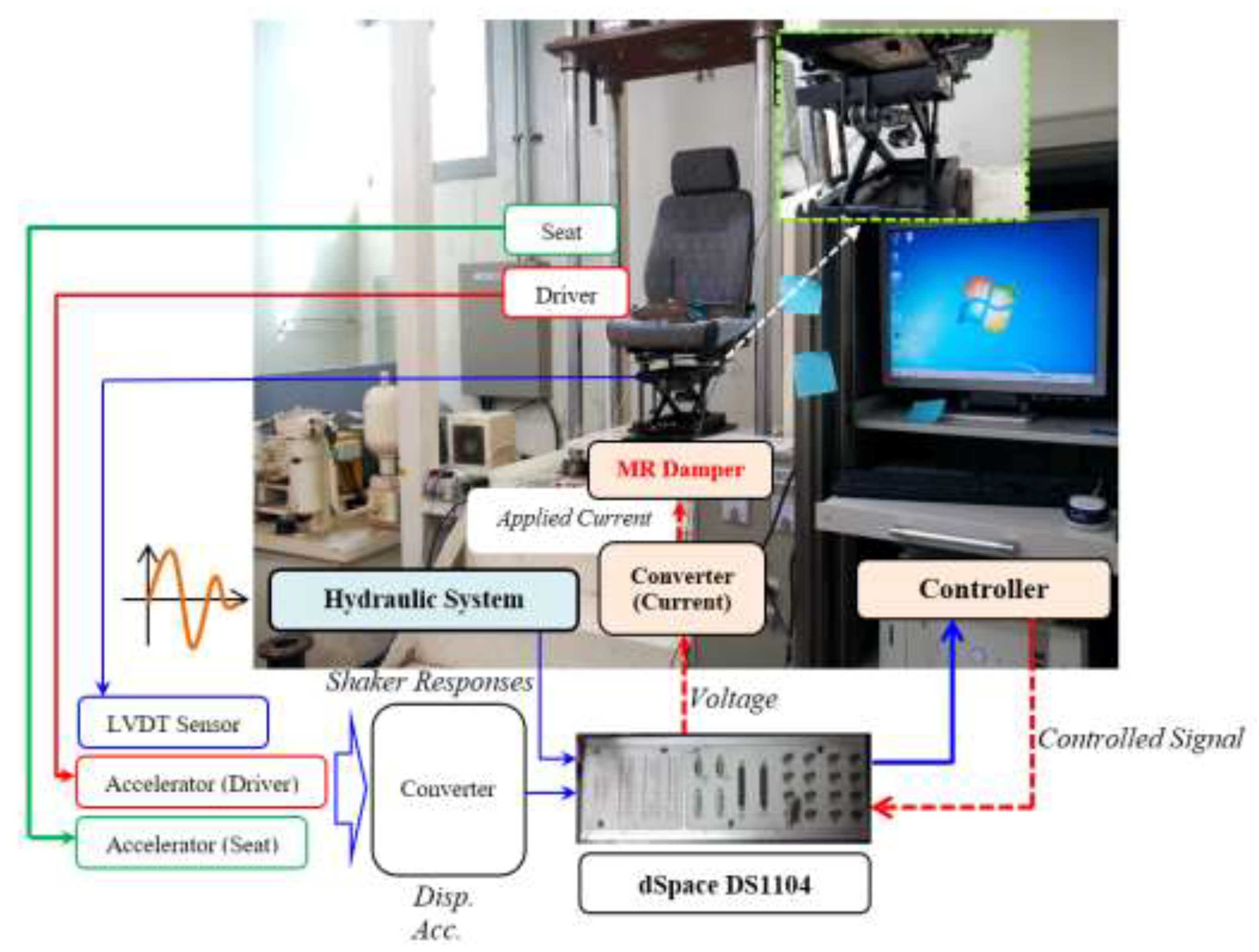
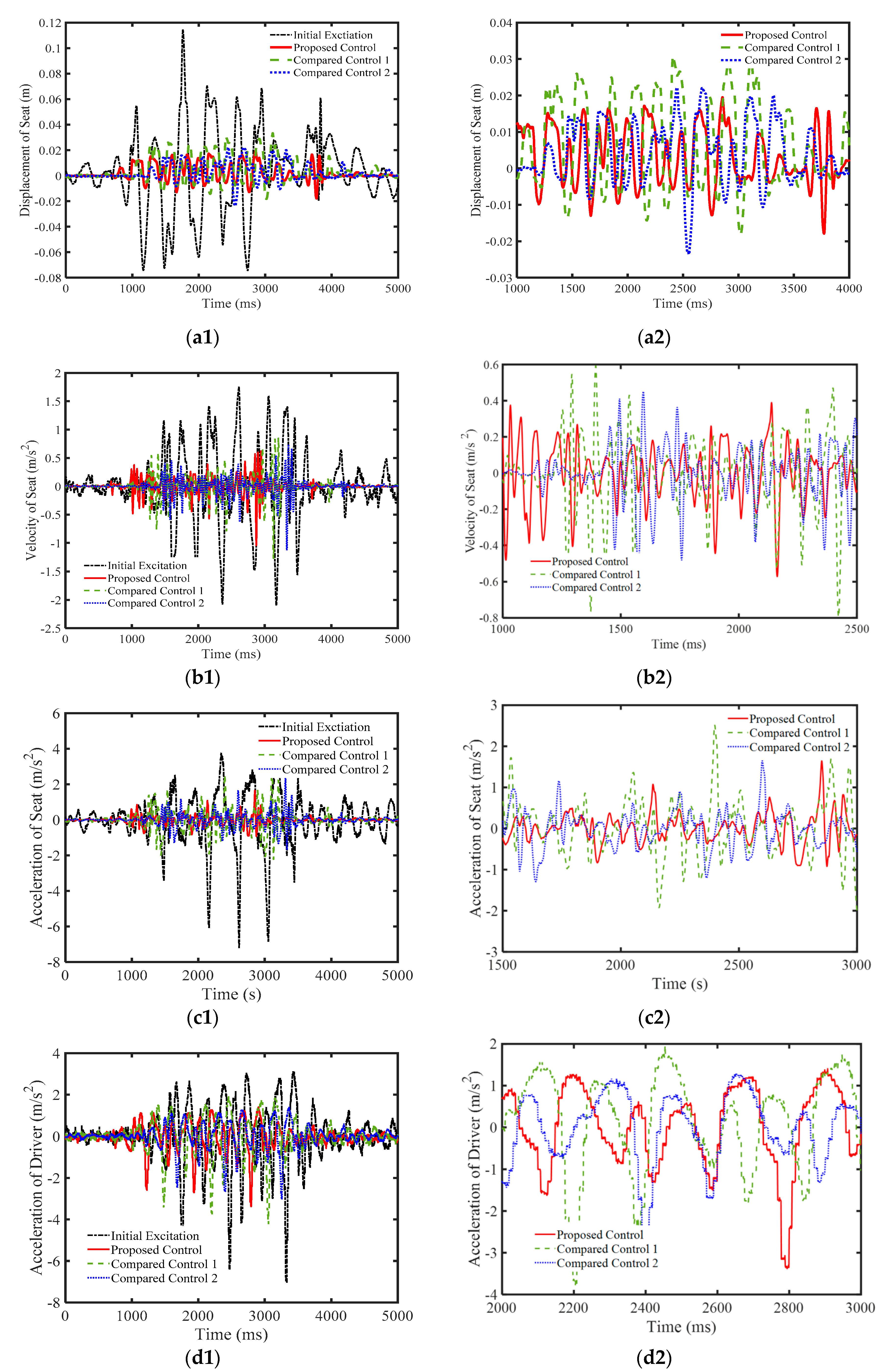
4. Experimental Results and Discussions

To implement the proposed controller, an experiment setup is shown in Figure 6, in which several sensors such as linear variable differential transformer (LVDT) transducer, accelerometers at the seat and driver were used to get the feedback signals to the controller. Detail information for the sensor is shown in [9]. In this experiment, two comparative controllers were adopted for comparison: Comparative Controller 1 [22] and Comparative Controller 2 [9]. These comparative controllers are the type of hybrid controller including the Riccati-like equations and the combination of sliding mode control and fuzzy control in their design. This choice is valuable for evaluating the proposed controller, which is also a kind of hybrid controller. As in the computer simulation, the random-step-wave road excitation was chosen for the experiment. This excitation was embedded in the shaker system, as shown in Figure 6. It is noteworthy that the computer system included two part: one for the hydraulic shaker control and the other for the proposed controller with Dspace 1104. The applied current for MR damper was used with maximum value 2 A for three controllers. The limitation of the maximum value of the applied current was reasonable to evaluate three controllers showing their best in control performance under severe vibration environment. The measured results of the controllers are presented in Figure 7, Figure 8 and Figure 9. In Figure 7, the responses of the controllers including displacement, velocity, and acceleration of seat and driver are shown. It is clearly seen that the proposed controller provides better vibration control performance than the comparative controllers [9,23]. The applied current of three controls are shown in Figure 8. In this figure, the input controls appear to be very complicated, but it is clear the maximum input current has been limited by 2A. Now, to more clearly observe the benefits of the proposed controller, the power frequency responses are presented in Figure 9. It is remarked here that, according to the standard ISO 2631-1, the acceleration at the driver position should be less than 2.5 m/s². It is seen in Figure 9a that three controllers are effective in control vibration, but the proposed controller clearly provides lower values than the other controllers [9,23]. Based on the decrease of the acceleration of the seat, the acceleration at the driver position is also decreased, as shown in Figure 9b. The acceleration of the proposed control and the comparative controller 2 [9] is nearly similar. This is originated from the damping ratio of the seat frame which is nonlinear. To compare three controllers, quantification was undertaken in this work: the performance of three controllers was continuously evaluated using the ToD (Transmissibility of Displacement) and ToA (Transmissibility of Acceleration) values of the seat [9]. The ToD values of the random step wave excitation were 0.213565, 0.358171, and 0.246641 for the proposed controller, Comparative Controller 1 [23], and Comparative Controller 2 [9], respectively. Similarly, from the acceleration responses, the ToA values of random step wave excitation were identified as 0.170182, 0.396618, and 0.257991 for the proposed controller, Comparative Controller 1 [23], and Comparative Controller 2 [9], respectively. From the above results, the proposed controller is the best, showing outstanding vibration control with the stability of the system under severe road disturbance.

5. Conclusions

In this study, a new controller using a new modified Riccati-like equation with three parameters of the PID controller was proposed and its effectiveness was validated from computer simulation and experimental realization. The robustness of the controller was improved using the sliding surface of sliding mode controller and the fuzzy neural networks model. The H_infinity technique was also used for connecting the above controller and the parameters of the Riccati-like equation. The stability of the proposed control was proven based on the Lyapunov stability criterion. The formulated controller was applied to vibration control of the vehicle seat suspension system with MR (magnetorheological) damper subjected to severe road excitations: random bump road and random step wave road. It was demonstrated that the proposed controller can bring control robustness, showing well-controlled unwanted vibrations at the seat and the driver position in terms of the displacement and accelerations. In addition, it was shown from comparative work that the proposed controller can provide the best vibration control performance compared two existing controllers, which are kinds of hybrid controllers designed for robustness guarantee of control system. The superior property of the proposed controller was also confirmed by calculating two factors of transmission: ToD and ToA. The results presented in this work are self-explanatory, justifying that the proposed controller can apply to any physical system subjected to disturbances and/or uncertainties. As a second phase work, a new robust controller will be formulated by considering both the variation of the main system parameters such as sprung mass and unmodeled dynamics of the driver such as human body model.

References

1. Bounemeur, A.; Chemachema, M.; Essounbouli, N. Indirect adaptive fuzzy fault-tolerant tracking control for MIMO nonlinear systems with actuator and sensor failures. ISA Trans. 2018, 79, 45–61. [Google Scholar] [CrossRef] [PubMed]
2. Davanipour, M.; Khayatian, A.R.; Dehghani, M.; Arefi, M.M. A solution for enhancement of transient performance in nonlinear adaptive control: Optimal adaptive reset based on barrier Lyapunov function. ISA Trans. 2018, 80, 169–175. [Google Scholar] [CrossRef] [PubMed]
3. Zhang, W.; Su, H. Fuzzy adaptive control of nonlinear MIMO systems with unknown dead zone outputs. J. Frankl. Inst. 2018, 355, 5690–5720. [Google Scholar] [CrossRef]
4. Moradi, M.; Fekih, A. Adaptive PID-sliding-mode fault-tolerant control approach for vehicle suspension systems subject to actuator faults. IEEE Trans. Veh. Technol. 2014, 63, 1041–1054. [Google Scholar] [CrossRef]
5. Cao, K.; Gao, X.; Lam, H.-K.; Vasilakos, A. H∞ fuzzy PID control synthesis for Takagi–Sugeno fuzzy systems. IET Control. Theory Appl. 2016, 10, 607–616. [Google Scholar] [CrossRef]
6. Chamsai, T.; Jirawattana, P.; Radpukdee, T. Robust adaptive PID controller for a class of uncertain nonlinear systems: An application for speed tracking control of an SI engine. Math. Probl. Eng. 2015, 2015. [Google Scholar] [CrossRef]
7. Mahmoodabadi, M.J.; Abedzadeh Maafi, R.; Taherkhorsandi, M. An optimal adaptive robust PID controller subject to fuzzy rules and sliding modes for MIMO uncertain chaotic systems. Appl. Soft Comput. 2017, 52, 1191–1199. [Google Scholar] [CrossRef]
8. Subramanian, R.G.; Elumalai, V.K.; Karuppusamy, S.; Canchi, V.K. Uniform ultimate bounded robust model reference adaptive PID control scheme for visual servoing. J. Frankl. Inst. 2017, 354, 1741–1758. [Google Scholar] [CrossRef]
9. Phu, D.X.; An, J.-H.; Choi, S.-B. A novel adaptive PID controller with application to vibration control of a semi-active vehicle seat suspension. Appl. Sci. 2017, 7, 1055. [Google Scholar] [CrossRef]
10. Van, M.; Do, X.P.; Mavrovouniotis, M. Self-tuning fuzzy PID-nonsingular fast terminal sliding mode control for robust fault tolerant control of robot manipulators. ISA Trans. 2019. [Google Scholar] [CrossRef]
11. Phu, D.X.; Choi, S.-M.; Choi, S.-B. A new adaptive hybrid controller for vibration control of a vehicle seat suspension featuring MR damper. J. Vib. Control. 2017, 23, 3392–3413. [Google Scholar] [CrossRef]
12. Phu, D.X.; Huy, T.D.; Mien, V.; Choi, S.-B. A new composite adaptive controller featuring the neural network and prescribed sliding surface with application to vibration control. Mech. Syst. Signal. Process. 2018, 107, 409–428. [Google Scholar] [CrossRef]
13. Do, X.P.; Nguyen, Q.H.; Choi, S.-B. New hybrid optimal controller applied to a vibration control system subjected to severe disturbances. Mech. Syst. Signal. Process. 2019, 124, 408–423. [Google Scholar]
14. Phu, D.X.; Hung, N.Q.; Choi, S.-B. A novel adaptive controller featuring inversely fuzzified values with application to vibration control of magnetorheological seat suspension system. J. Vib. Control. 2018, 24, 5000–5018. [Google Scholar]
15. Li, Y.; Zhang, H.; Liang, X.; Huang, B. Event-triggered-based distributed cooperative energy management for multi-energy systems. IEEE Trans. Ind. Inform. 2019, 15, 2008–2022. [Google Scholar] [CrossRef]
16. Zhang, H.; Li, Y.; Gao, D.W.; Zhou, J. Distributed optimal energy management for energy internet. IEEE Trans. Ind. Inform. 2019, 13, 3081–3097. [Google Scholar] [CrossRef]
17. Li, Y.; Zhang, H.; Huang, B.; Han, J. A distributed Newton–Raphson-based coordination algorithm for multi-agent optimization with discrete-time communication. Neural Comput. Appl. 2018, 1–15. [Google Scholar] [CrossRef]
18. Wang, X.; Liu, X.; Zhang, L. A rapid fuzzy rule clustering method based on granular computing. Appl. Soft Comput. 2014, 24, 534–542. [Google Scholar] [CrossRef]
19. Mendel, J.M. Computing derivatives in interval type-2 fuzzy logic systems. IEEE Trans. Fuzzy Syst. 2004, 12, 84–98. [Google Scholar] [CrossRef]
20. Juang, C.-F.; Chen, C.-Y. Data-driven interval type-2 neural fuzzy system with high learning accuracy and improved model interpretability. IEEE Trans. Cybern. 2013, 43, 1781–1795. [Google Scholar] [CrossRef]
21. Liang, Q.; Mendel, J.M. Interval type-2 fuzzy logic systems: Theory and design. IEEE Trans. Fuzzy Syst. 2000, 8, 535–550. [Google Scholar] [CrossRef]
22. Ciccarella, G.; Dalla Mora, M.; Germani, A. A Luenberger-like observer for nonlinear systems. Int. J. Control. 1993, 57, 537–556. [Google Scholar] [CrossRef]
23. Wu, T.-S.; Karkoub, M.; Wang, H.; Chen, H.-S.; Chen, T.-H. Robust tracking control of MIMO underactuated nonlinear systems with dead-zone band and delayed uncertainty using an adaptive fuzzy control. IEEE Trans. Fuzzy Syst. 2017, 25, 905–918. [Google Scholar] [CrossRef]
Figure 1. Mechanical model of the seat suspension with MR damper.
Applsci 09 04540 g001
Figure 2. Simulation results of displacement of seat under random bump road excitation: (a,b) general view; and (c,d) large view.
Applsci 09 04540 g002aApplsci 09 04540 g002b
Figure 3. Simulation result of power spectral density of displacements under random bump road excitation.
Applsci 09 04540 g003
Figure 4. Simulation results of displacement of seat under random step wave road excitation: (a,b) general view; and (c,d) large view.
Applsci 09 04540 g004aApplsci 09 04540 g004b
Figure 5. Simulation result of power spectral density of displacements under random step wave road excitation.
Applsci 09 04540 g005
Figure 6. Experiment setup of seat suspension with MR damper for a commercial bus.
Applsci 09 04540 g006
Figure 7. Experiment results under random-step-wave excitation: (a1) displacement; (a2) large view of the displacement; (b1) velocity; (b2) large view of the velocity; (c1) acceleration at the seat; (c2) large view of the acceleration at the seat; (d1) acceleration of the driver; and (d2) large view of the acceleration of the driver.
Applsci 09 04540 g007
Figure 8. Applied current of random-step-wave excitation: (a) general view; and (b) large view.
Applsci 09 04540 g008
Figure 9. Experiment results of power spectral density: (a) acceleration of seat; and (b) acceleration of driver.
Applsci 09 04540 g009