Numeric Evaluation of Game-Theoretic Collaboration Modes in Supplier Development

Featured Application

In the context of supplier development we developed four different possibilities of manufacturers’ information exchange to investigate the profitability of supplier development under cooperation, collaboration and non-cooperation strategies based on dynamics supplier development contracting.

Abstract

To deal with increasingly competitive challenges, today’s companies consider supplier performance as a crucial factor to their competitive advantage. Supplier development is one of the recent approaches to supplier performance enhancement and consistently requires relationship-specific investments. It is important to invest money, experts and/or machines in a supplier to minimize the risk of an inefficient supply chain while maximizing the level of profitability. This paper provides the number of optimization models to confront this issue utilizing Model Predictive Control. We consider a centralized and distributed setting with two manufacturers and one supplier, which enables us to simulate more realistic scenarios. We implement cooperative and non-cooperative scenarios to assess their impact on the manufacturers’ revenue. Results reveal that the cooperative setting between manufacturers pays off better than non-cooperative and collaborative settings in long-term investments. However, for short-term investments, the non-cooperative setting performs better than the others. We can conclude that, in short-term supplier development investments, an added value is generated since both the manufacturers and the supplier gain flexibility, therefore, investing separately can end up with higher profit for both manufacturers.

1. Introduction

Manufacturing companies confront procurement costs of raw materials and components of over 50% of the companies’ total profit [1,2]. As a result, manufacturers depend on their suppliers, and the suppliers performance shows a considerable effect on many product aspects, such as cost, quality, and on-time delivery [2]. Consequently, manufacturers place increasing concentration on a more efficient supply chain utilizing supplier development.

The purpose of supplier development is enhancing the performance and/or potentials of the supplier to fulfill the supply needs of manufacturers, such as improvement in response to customer needs and market dynamics, increasing customer responsiveness, improvement of quality and reliability of products, manufacturing of new products, reducing costs of production and then ultimately, to increase profit margins [2,3,4]. Hence, it is in the interest of manufacturers and suppliers to seek competitive advantages through supplier development.

According to the relational perspective, manufacturers invest in supplier development to gain tangible profits like lower cost, higher quality and flexibility, and trustworthy delivery. In these cases, the manufacturer, to achieve the better performance and shared value development, may be determined to support the supplier via information exchange, technological support, training, and through investiture in supplier processes [5].

Supplier development can provide the foundation of cooperation among buyers and suppliers. However, supplier development offers the chance of collaboration among several manufacturing companies as well. Many manufacturing companies, especially the ones that are active in the same industry, tend to order raw materials and components from an assortment of suppliers. As an instance, Whirlpool and General Electric for washing machines’ motors, Toyota and Pontiac for automobiles’ engines and Dell and Hewlett-Packard for personal computers’ PC boards work with the same suppliers [2]. Generally, in such a situation, a manufacturer can choose between various types of relationships, which can be cooperative, non-cooperative, and collaborative [6].

In this paper, we study multi-manufacturer scenarios, which consist of two manufacturers and one supplier to enable us to simulate more realistic settings. We assume four types of relationships between manufacturers that are fully cooperative, collaborative (simultaneous and sequential decision-making) and non-cooperative. Previous studies suggest a wide range of definitions for the cooperative and collaborative relationship in supply chains. In this study, we assume a cooperative relationship where partners act together to achieve a shared goal. In contrast, in a non-cooperative scenario, manufacturers aim to maximize their profit. Furthermore, manufacturers in collaborative relationships generally aim to maximize their own profit, while rendering their decisions separate from each other. We subdivide the collaborative setting in terms of the order of decisions. In a simultaneous setting, both manufacturers make their decisions at the same time, while constantly forwarding their decisions to the other manufacturer. In a sequential setting, one manufacturer makes its decision first and reveals it to the second manufacturer.

In this paper, we investigate the effect of centralized and distributed relationships between manufacturers on the overall profit of the supply chain. Furthermore, we attempt to answer the following questions: Are collaboration, cooperation, and non-cooperation good scenarios for manufacturers who intend to develop the same supplier by means of dynamic horizon investment? How can cooperative, collaborative, and non-cooperative settings between manufacturers affect the profit of the supply chain in short-term investments?

To answer the mentioned questions, we expand the scenarios of [7,8] from a monopolistic setting (one manufacturer–one supplier) to a multi-manufacturer setting with two manufacturers and one supplier. Then, we consider different types of relationships between manufacturers to find out which one works efficiently. In order to conduct this study, we apply a Model Predictive Control (MPC) to model and optimize the profit of supply chain [7]. MPC combines short-term closed-loop control with a long-term open-loop simulator/optimizer. It implements optimization over long-term model-based simulations to determine an optimal control sequence, which represents the planned investments undertaken by the manufacturers for that period.Due to turbulent and complex environment in today’s manufacturing, long-term investments are usually not secure and reasonable, and manufacturers should be more agile to react to the changes in the market in order to survive. Therefore, for the first time in the field of supplier development, we apply the MPC method to find the optimal horizon of supplier development investment considering different relationship scenarios between manufactures. Relying on the result of this study, decision makers will be able to choose whether they are willing to extend the investment on supplier development programs or not.

The contributions of this paper are multi-fold. First, we seek to model cooperative, non-cooperative, and collaborative supplier development scenarios as a game-theoretic, analytic evaluation. These models provide insights into how two manufacturers are investing in supplier development and how this investment will affect their revenue. Here transfer the profit function for supplier development from [7,8] into different manufacturer relationship settings to investigate the impact of revenues to scale on investment strategies. Application of mathematical models in general and of control theory particularly is increasing in supply chains decision-making [7]. Among them, model predictive control (MPC), also called receding horizon control, is of particular interest as it ables us to cope with non-linear constrained multi-input multi-output problems as well as key performance criteria, cf. [9] for details. The method itself is a well-established simulation strategy to deal with uncertainties in supply chains, see, e.g., [10], and was used in [7] for supplier development to reduce the drawbacks of contracts utilizing dynamic contract extensions.

The remainder of the paper is structured as follows: First, the background of this study is shortly reviewed in Section 2. In Section 3, the optimizing method(Model Predictive Control) is described. In Section 4, the model formulation to determine the profit of supplier development is explained, and manufacturers and supplier cost parameter are detailed. In the final Section 5 and Section 6, results and discussion are drawn.

2. Related Literature

We study the effect of different interactions between manufacturers on the profit of supplier development. Therefore, it is essential to investigate the literature of supplier development and different possibilities of information exchange precisely. Following we divide the previous studies into two main subjects supplier development and game theory.

2.1. Supplier Development

In the past decades, many supplier development studies have been conducted [2,11,12,13,14,15]. Former researches provided deep insights into the propagation of supplier development in applications [11] applying specified operations in the supplier development context [12], the important success elements [13], and the key issues in sustainable supplier development partnership [15]. Additionally, in various industries, supplier development has been utilized. In the automotive industry, Toyota started preparing on-site support to include suppliers into the Toyota Production System [2]. Subsequently, Boeing, Chrysler, Daimler, Dell, Ford, General Motors, Honda, Nissan, Siemens, and Volkswagen followed this collaborative procedure to enhance their suppliers’ performance [14].

In the context of supplier development, Talluri et al. [2] developed two scenarios: a single manufacturer and multiple suppliers ($SMMS$) and two manufacturers and multiple suppliers ($TMMS$). They investigated long-term investment in supplier development. In their $TMMS$ model, they assume that when manufacturers cooperate in supplier development, they can gain benefits of the other company’s investment. In a cooperative situation, both manufacturers confront the same level of “shared risk”. While in a non-cooperative case a manufacturing company’s can only gain benefits of its investments.

Dale et al. [15] studied the effect of long term relationship on the result of supplier development. According to their study, effective partnership requires treating suppliers as long-term business partners, and this needs a basic transmission from the conventional adversarial buyer–supplier relationship to the long term relationships and connections between buyer–supplier. They showed that a properly implemented partnership will contribute to reduce costs and increase market share to the benefit of both parties, together with technology transfer issues surrounding product, process, practices, and systems. Finally they provided a list of actions which should/should not be taken in order to support both manufacturers and suppliers to establish a kind of partnership that is most proper for them.

Bai and Sarkis [6] applied different game-theoretic scenarios to investigate the effect of various interactions of manufacturers and suppliers on the profit of supplier development. The results illustrate that engaged partners in supplier development can gain more benefits than non-cooperative relationship. They also revealed that a cooperative situation needs more resource and knowledge investment. They conducted their study based on a long term supplier development contract. In the present study, we take one step further and consider the effect of dynamic supplier development contracting on overall profit over the various relationships between manufacturers.

Kumar and Routroy [16] conducted an applied survey in Indian manufacturing industry to investigate the interactions among the impediments to supplier development programs. Their study comprehensively combined the prominent impediments which emerge from different aspects such as supplier, manufacturer, manufacturer-supplier. They aimed to provide a foundation for a manufacturer to effectively conduct supplier development programs. Moreover, they established that the collaborative operations such as, collaborative planning, collaborative decision making and collaborative execution of supply chain plans facilitate a high level of success in the collaborative supply chains. They also modeled the relationship among the collaborative operations, success of collaboration and long-term future collaborations.

Glavee-Geo [17] tried to find how supplier development causes supplier satisfaction. Therefore, he developed and examined a model utilizing the PLS variance-based modeling method, and carried a post-hoc analysis utilizing the polynomial regression procedure. The results of his study revealed that supplier development is an essential means by which manufacturer can improve supplier satisfaction. He showed that supplier development remarkably anticipates the future of business relationships. Moreover, the result of the analysis showed a considerable positive influence of supplier development on the two dimensions of supplier satisfaction, which were, economic and non-economic satisfactions, and presented notable effects on both aspects.

To investigate the interactions of manufacturers and suppliers in the supply chain, researchers considered different possible settings as mentioned above, which, comprehensively, can be regarded as Cooperation, Coordination, and Collaboration. According to the mentioned strategies, previous studies refer to the supply chain’s partnerships as coordinative, cooperative, or collaborative in nature and behavior [18].

In the current study, we investigate the effect of different manufacturer-to-manufacturer relationships on the revenue of supplier development in both short-term and long-term investment. Thereby, we assume that both manufacturers profits from supplier investments, no matter who conducted the investment. We aim to determine the level of profitability of supplier development investments in different interactions, such as cooperative, collaborative, and non-cooperative gaming situations. Specifically, we investigate a wider range of relationships than previous studies, to identify which gaming situations, are more profitable. We study a two-manufacturer and one-supplier scenario. When two manufacturing companies target one supplier in their supplier development efforts, they can choose cooperate, collaborate, or non-cooperate relationships. Each of these options has its benefits and drawbacks. The benefit of not cooperating is that the manufacturer can develop unique elements with aspects that cause different advantages from its competitors. However, companies still should deal with all of the risks of supplier development and may require to invest more to achieve the same returns.

While, in cooperative investment on the same supplier, both manufacturers can share their resources, and therefore they need less effort, and for the greater volume, they both can enjoy economies of scale. However, working with the same supplier causes equality of the manufacturers’ products, companies still have the chance of generating differentiation on other aspects of their products. As an instance, BMW cars may look and work differently from a Mercedes, even if they purchased the same electric window opener from Bosch.

As can be seen, most researches deal with the relationship among manufacturers and suppliers in the context of supplier development. Nevertheless, all of researchers assume a fixed long-term supplier development program as a baseline. In this research for the first time we apply dynamic supplier development contracts to investigate the profitability of different relationships among partners in supply chain. From a dynamic investment perspective we are able to gain better insights into manufacturers relationships in mid-term and short-term supplier development programs. Therefore, we adopt four types of communication based on game theory in the context of supplier development and utilize model predictive control. Using model predictive control we are able to find an optimal investment horizon for both manufacturers. Therefore, based on the most profitable investment horizon decision makers can decide whether they continue to invest on supplier development or not.

2.2. Types of Games in Game Theory

In the literature of game theory, many researchers suggested different classifications of games; here, we provide a summary of former studies, to achieve a better understanding of different features of games to distinguish different ways of communications between manufacturers.

2.2.1. Cooperative and Non-Cooperative Games

In a cooperative game, players can pick a particular strategy and form commitments through negotiations and agreements among players. However, in non-cooperative games, any negotiations and agreements are not possible [19,20,21]. In cooperative games, players can play as a team with common goals. However, in non-cooperative games, players can keep their unities, and are able to choose their strategy to maximize their revenue [22,23,24].

2.2.2. Symmetric and Asymmetric Games

The payoff of a symmetric game does not depend on the player. Indeed, it depends on the adopted strategy. It means the decisions for all players stay the same without changing the results of the strategies [25]. In other words, the dominant strategy of the game is uniform for all players [21,26].

2.2.3. Zero-Sum and Non Zero-Sum Games

Zero sum games are the situations where one or more players’ gain (loss) equals the loss (gain) of other players. Therefore, a gain (loss) for one must result in a loss (gain) for one or more others, which simply means one player gains the equal amount that its opponent losses [27,28]. On the other hand, when the final result of all players is not zero, the game is anon-zero sum game [24,29].

2.2.4. Simultaneous and Sequential Games

In simultaneous games, also called static games, players undertake their moves at the same time. Thereby moves are considered an adaptation of a strategy that, the player decided for [27]. In simultaneous games, players do not have information about the decisions of other players [29,30]. In contrast, in sequential or dynamic games, players are informed about the decision of the other player who has already started the game.

2.2.5. Perfect Information and Imperfect Information Games

In a perfect information game, all players are aware of the other players’ decisions. Therefore, among the mentioned games, only sequential games fit in this category [31]. Almost all types of gaming are in the class of imperfect games instead of sequential games [32].

Following these definitions of different games, the remainder of this article proposes a formulation of four different interaction scenarios based on model predictive control. These allow us to assess the efficiency of supplier development in a multi-manufacturer and one supplier setting.

3. MPC Control Scheme

The MPC scheme is particularly useful to model and optimize systems, where decision-makers, in this case, manufactures, can utilize different portions of information about the real-world system (about the supplier and their competitors). While the measured state contains all information about all the manufacturers’ activities in the last time step, the corresponding system models can be defined to only include knowledge available from the respective kind of cooperation or collaboration. Therefore, the (open loop) simulation is restricted to only use information applicable for the specific setting to make a decision, while the effects of all independent decisions can be integrated using the measurement of the current (closed-loop) real-world system state. As a result, each setting is defined by three different components:

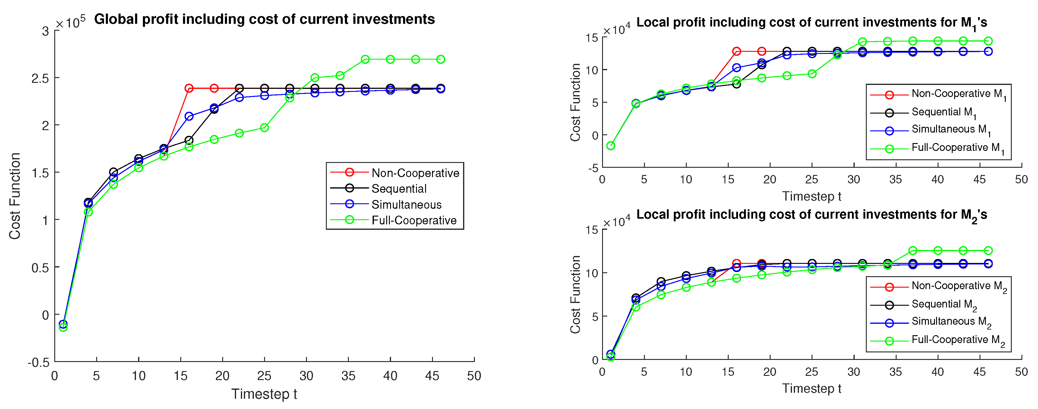
• Cost function: The cost function of each scenario differs in whether the manufacturers pursue a common goal or try to obtain their respective profit.
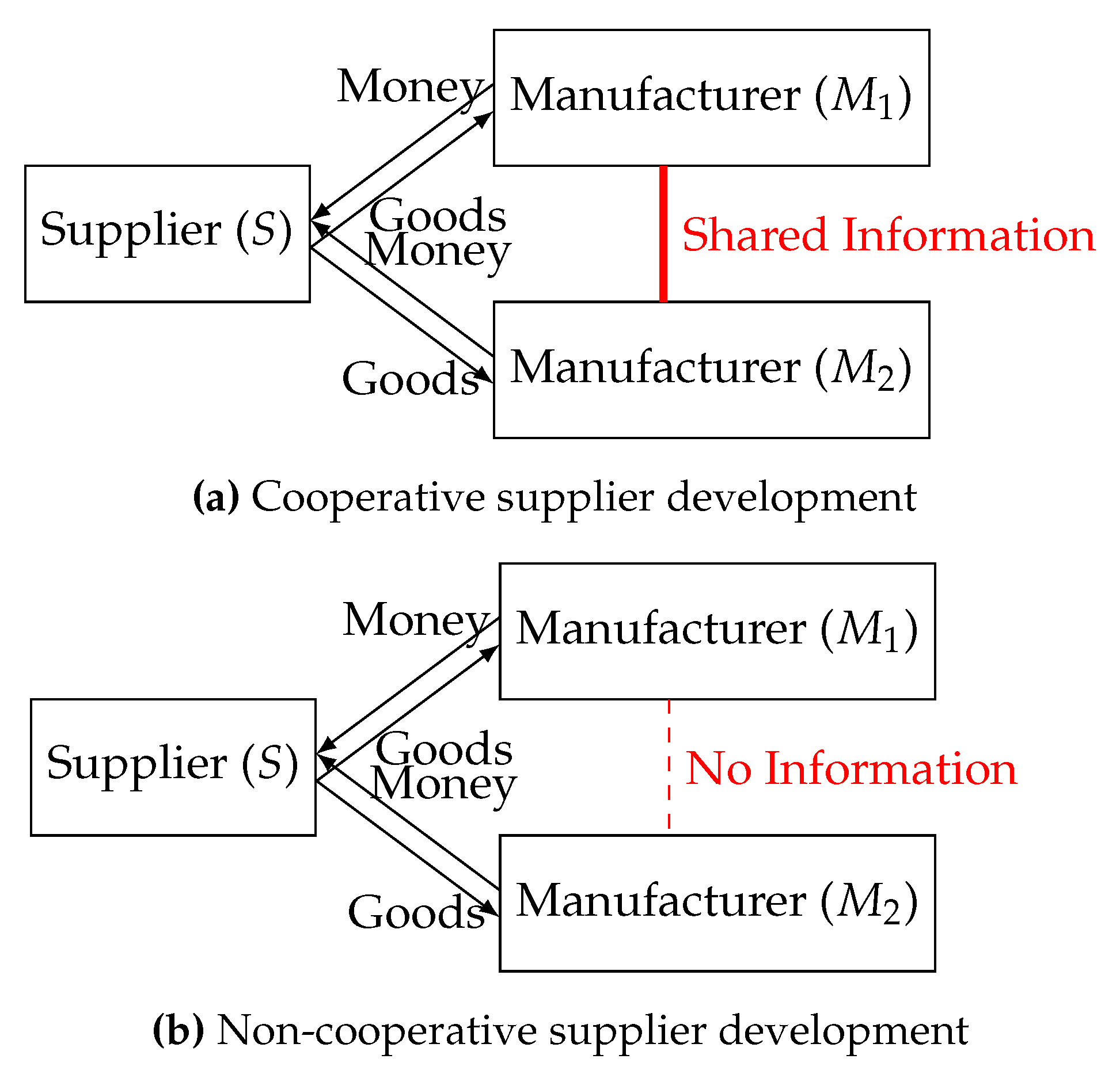
• System model: Depending on the scenario, the system model can differ strongly. For example, in the full cooperation setting, a common system model can be used, which includes all information about both manufacturers. In contrast, the non-cooperation setting uses two fully separate system models as neither manufacturer has any information about the other.
• Order and sequence of decision-making: In particular the sequential and simultaneous settings rely on different orders of decision making steps within each time step. For instance, multiple decision-making iterations can be used to represent the sharing of information. Thereby, each manufacturer makes a decision and conveys this decision to the other one. The latter uses the mentioned information to render its own decision and replies back to the first manufacturer. Now, the first manufacturer can again use the newly acquired information to update its decision and so on. As a result, several cycles of decision making can be part of a single time step.

MPC consists of control parts, which applies short-term control decisions to the real-world system and receives feedback about respective effects, and an open-loop simulation, which acts as the foundation for the long-term optimization. Figure 1 sketches the overall scheme, where the real-world system is shown on top of the figure, which refers to the two manufacturers and a supplier. The real-world system receives control inputs from the closed-loop control at predefined time steps $t_i$, $i\in 1,\dots ,N$ and provides a measured state of the system $x_n$, $x_n\in x_0,\dots ,\left(x_N\right)$ and a measured time step $t_m$, $t_m\in t_0,\dots ,\left(t_N\right)$ to the closed-loop control. In this study, we assume a 5 years supplier development project and compute the optimal profitability by applying the 3-month intervals ($\Delta t=3$), which means $N=20$. The closed-loop control uses this information to initiate an open-loop simulation-based optimization. In contrast to the closed-loop, the open-loop covers an increased time horizon of N time steps. The effects of control decisions $u_i$ with $i\in t_m,\dots ,t_N$ are simulated using an underlying system model and the control sequence $u_{t_m},\dots ,u_{t_N}$ is optimized using a provided cost function. The latter is not shown in the picture but is assumed to be part of the optimization. The obtained optimal control sequence for N time steps is then returned to the closed-loop control, which forwards the first element of this sequence $u_{t_m}$ to the real-world system as control decision for the current time step. After application, a new measurement is conveyed to the closed-loop control and the overall cycle restarts.

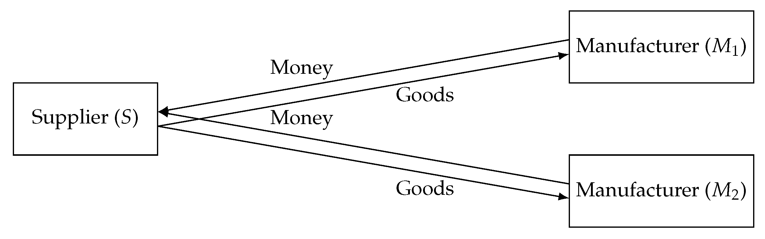
4. Model Description

In this paper, we expand the setting from [7] to a multi-manufacturer structure, which consists of two manufacturers $M_1$ and $M_2$ and a single supplier S, cf. Figure 2.

While S provides components to $M_1$ and $M_2$, manufacturers assemble these components to final products and sell these to the market. We assume that $M_1$ and $M_2$ dominate the market and determine the number of final products to maximize profit. To this end, $M_1$ and $M_2$ increase/decrease market demands by decreasing/increasing the product sale price. This study is based on the assumption that the product sale price for both of the manufacturers are equal. The focus lies on an asymmetric reliance on the supplier (higher $c_S$ for one). Including advanced pricing strategies would make the results incomparable as we cannot determine which mechanism leads to the results. Further, it is assumed that the supplier is an exclusive one and also both manufacturers gain the same profit from their investment. In order to study different relationship settings, we introduce the model for a symbolic manufacturer M instead of considering two manufacturers $M_1$ and $M_2$. Later we discuss how manufacturers shape different types of relationship and how relationships can affect the overall profit of supplier development.

4.1. Derivation of the Optimizer’s Cost Function

Here, we consider a linear price distribution curve $p\left(d\right)=a-b·d$, where d represents the production quantity and p represents the sale price, cf., e.g., [7,33,34,35], and where $a>0$ and $b>0$ signify the prohibitive price and the price elasticity of the production. In the present study, prohibitive price is the maximum price of the manufacturer’s products that consumer can afford and the price elasticity is the range of product’s price that the supplier offers to the manufacturer.

Note that this system shows only one decision variable, which is given by the sales of the manufacturer. The supplier cannot take a decision with regards the production quantity and just produces the components to meet the market demand d. Due to revenue maximization, the production quantity d which adopted by M is determined by the zero of the first derivative of the profit given by $d(p\left(d\right)-c_{\mathrm{M}}-c_{\mathrm{SC}})$, where $c_{\mathrm{M}}$ and $c_{SC}$ denote the unit production costs of M and the supply costs per unit of S, cf. [7,8]. Hence, we obtain

$$\begin{array}{c}\hfill p\left(d\right)-c_{\mathrm{M}}-c_{\mathrm{SC}}-bd=0\end{array}$$

and thereby the optimal production quantity and optimal sale price

$$\begin{array}{c}\hfill d^{★}=\frac{a-c_{\mathrm{M}}-c_{\mathrm{SC}}}{2b},p\left(d^{★}\right)=\frac{a+c_{\mathrm{M}}+c_{\mathrm{SC}}}{2}\end{array}$$

In order to include fixed revenues per unit r of the supplier S similar to [7,8,33,34,35], we define $c_{\mathrm{SC}}:=r+c_{\mathrm{S}}$, where $c_{\mathrm{S}}$ represents the unit production costs of the supplier S. Now, we maximize the overall profit J, which is the summation of manufacturer profit $J^M$ and the supplier profit $J^S$

$$\begin{array}{c}\hfill J\left(c_{\mathrm{S}}\right)=J^M\left(c_{\mathrm{S}}\right)+J^S\left(c_{\mathrm{S}}\right)=\frac{{(a-c_{\mathrm{M}}-c_{\mathrm{SC}})}^2}{4b}+\frac{a-c_{\mathrm{M}}(r+c_{\mathrm{S}})}{2b}r.\end{array}$$

Greater experience or development in human resource capabilities, production process or machines enable the supplier to improve its capability. Learning causes less effort and time, and in turn also fewer production costs per unit. To formulate the problem more realistic, we take the supplier learning rate into account. We suppose that the manufacturer wants to increase the overall revenue of the supply chain by decreasing the unit production costs $c_{\mathrm{S}}$ of the supplier via supplier development projects. To this end, we introduce a time-dependent function $x:\mathbb{R}\to \mathbb{R}$

$$\begin{array}{c}\hfill c_{\mathrm{S}}=c_{0}x{\left(t\right)}^m,\mathrm{with}\dot{x}\left(t\right)=u\left(t\right),x\left(0\right)=x_0=1\end{array}$$

where $c_0>0$ represents the base unit production cost of the supplier S, and $m<0$ characterizes its learning rate. Last, x donates the number of supplier development projects, which can be changed by the manufacturer M via $u\in [0,\omega ]$. The bound $\omega >0$ to represents a resources availability limitation, which may be due to time, manpower, or budget. A variety of former studies have proposed similar models of cost reduction through learning, cf., e.g., [33,34,35,36]. To account for the respective development projects, we integrate supplier development costs $c_{\mathrm{SD}}u\left(t\right)$ into the profit function and obtain

$$J_T(u;x_0)=\underset{0}{\overset{T}{\int }}\frac{{(a-c_{\mathrm{M}}-c_{0}x{\left(t\right)}^m)}^2-r^2}{4b}-c_{\mathrm{SD}}u\left(t\right)dt,$$

(1)

where $c_{\mathrm{SD}}\ge 0$ represents the costs of a supplier development action. To have a more realistic setting, we do not consider problem parameters to be deterministic but some to be stochastic. While parameters such as the learning rate m are definitely stochastic and time-varying, parameters like the contract period T are most likely deterministic and fixed.

4.2. Settings

In the proposed multi-manufacturer and a single-supplier structure, we include the relationship of the manufacturers. Manufacturers have different options for communication to contract their supplier development investment. Regarding the game theory settings mentioned in Section 2, manufacturers are able either to invest in a supplier together (cooperative game) or to invest in a supplier individually (non-cooperative). In the latter case, they can choose between deciding on investing at the same time or sequentially. Note that our strategy in this setting is a non zero-sum game since utilizing manufacturers’ investment; both will gain profit regardless of the imposed strategy. Previous studies categorized and defined the relationships among partners in the supply chain in different ways [37,38,39,40]. In this study, for the first time, we adopt these four types of relationship based on game theory in the background of supplier development from a dynamic investment perspective. These different communication methods focus on the procedure of information sharing for supplier investment decision making. As an instance, in the full-cooperation setting, manufacturers share all information about their investment strategies and their supplier development programs with each other and pursue the shared goal to maximize their overall profit, cf. Figure 3a. The non-cooperative setting describes partners who tend to work separately without any communication, as outlined in Figure 3b. Collaboration means that the manufacturers contribute to develop the supplier while they are seeking to increase their profit out of the investment.

Nevertheless, the partners still try to maximize their key performance indicators. In these settings, partners can share information during a decision making step (simultaneous setting), shown in Figure 4a, or they can share their final decisions (sequential setting), shown in Figure 4b. Apart from using different system models, the scenarios differ in which parts of the vector u are optimized by the different manufacturers.

4.2.1. Cooperative Supplier Development

In cooperative supplier development, manufacturers work or act together to achieve a common goal. An explicit example of such a case is a joint venture supplier development project. In these types of shared projects, two cooperative manufacturers enter into a joint venture agreement by two different business entities for a supplier development project. The engaged parties share management, profits, and losses. Utilizing joint ventures enables manufacturers to combine resources or expertise. Therefore, they can save money in the development of a supplier [41]. In our scenario, manufacturers consider integrated profit as a key performance indicator. According to the outlined cooperative setting, manufacturers follow a common goal, consider the same system model, and render decisions simultaneously. In terms of game theory, this scenario can be considered a cooperative, symmetric, simultaneous game with complete information. In this study $u_1$ and $u_2$ represent the number of projects that $M_1$ and $M_2$ plan to conduct to develop their supplier.

In the cooperative scenario, a single, joint cost function $J(u_1,u_2;x_0)=J^{M_1}(u_1;x_0)+J^{M_2}(u_2;x_0)$ is used. Accordingly, only a single optimization run is performed, to optimize $u_1$ and $u_2$ together, that aim to the global optimum over both manufacturers. The open-loop system model is given as $x\left(t\right)=x(t-1)+u_1+u_2$ to represent that all information about both manufacturers is available.

4.2.2. Collaborative Supplier Development

In the collaboration setting, manufacturers seek to optimize their own goals and to gain more advantages from supplier development. They tend to share information about their investment with each other. In this study, the collaborative setting is broken down into two different settings, simultaneous and sequential decision making. In both cases, the scenario can be considered a cooperative, symmetric game with either perfect or imperfect information. As a consequence, two distinct system models are used in these scenarios. As each manufacturer aims to maximize its profit, two distinct optimization runs are performed, either optimizing $u_1$ for the first manufacturer or $u_2$ for the second.

Manufacturers may tend to make a decision with their partners simultaneously, which causes to apply the same system model for both manufacturers. Nevertheless, each manufacturer only decides on (optimizes) its actions $u_i$. To model the interactions in form of negotiations, the decision-making process is performed iteratively. Therefore both manufacturers first make a decision and share it with the other one. Using this new information, both parties revise their decision and again, communicate their new decisions until a maximum number of iterations is reached or no more changes in the decisions occur. Within the loop every manufacturer solves the corresponding optimization problems ($J^{M_1}(u_1;x_0,u_2)$ for $M_1$ and $J^{M_2}(u_2;x_0,u_1)$ for $M_2$) and updates the value for $u_i$. Accordingly the system model for both manufacturers is given as $x\left(t\right)=x(t-1)+u_1+u_2$.

In sequential decision making, one manufacturer makes a decision about its investment first and lets the other one know about it. Therefore it optimizes $J^{M_1}(u_1;x_0)$ using the open-loop system model $x_1\left(t\right)=x_1(t-1)+u_1$. Consequently, the second manufacturer can consider this information during its decision making, i.e., to optimize its profit as $J^{M_2}(u_2;x_0,u_1)$ using its own system model $x_2\left(t\right)=x_2(t-1)+u_1+u_2$. Therefore, the first manufacturer’s plan is available within the open-loop simulation of the second and the optimizer may identify the optimal investment plan, which causes the highest profit for the second manufacturer.

4.2.3. Non-Cooperative Supplier Development

In the non-cooperative setting, manufacturers look for their own goals and do not share any information about their supplier development program. This setting mostly occurs in highly competitive markets. Therefore, each manufacturer only optimizes over its own $u_i$, in this case, even without the knowledge about the other manufacturer’s decisions. Therefore, both manufacturers optimize their respective cost function $J^{M_i}(u_i;x_0)$ using the system model $x_i\left(t\right)=x_i(t-1)+u_i$. In terms of game theory, this scenario can be considered a non-cooperative, asymmetric game with imperfect information. From the MPC point of view, both manufacturers have their separate system models.

5. Results

In this section, we are particularly interested in the impact of manufacturers relationships on their revenue on supplier development. To this end, we utilize the MPC method to find the optimal profit of supplier development. The values of the parameters for an academic example from [8] are shown in

Table 1. List of parameters (Worthmann et al. 2016  [7]; Proch et al. 2017  [8]).

Symbol	Description	Value
T	Contract period	60
m	Learning rate	$-0.1$
a	Prohabitive price	200
b	Price elasticity	0.01
$c_{M_1}$	Variable cost per unit ($M_1$)	65
$c_{M_2}$	Variable cost per unit ($M_2$)	70
$c_0$	Variable cost per unit (S)	100
$c_{S{D}_1}$	Supplier development cost per unit ($M_1$)	9000
$c_{S{D}_2}$	Supplier development cost per unit ($M_2$)	8500
$u_1$	Number of supplier development projects ($M_1$)	[0, 5]
$u_2$	Number of supplier development projects ($M_2$)	[0, 2]

. We utilize these variables in (1) to compute the corresponding output values of profit $J_T(u;x_0)$ for all of the described settings.

We first compute the investment schema of $M_1$ and $M_2$ over time by using MPC in a Matlab framework. We apply an interior point gradient-based method to find the local optimum solution.

Solving the respective problems, we obtained Figure 5 and Figure 6. We observe that manufacturers in a fully cooperative setting tend to invest for longer periods than the others, and the manufacturers experience faster and greater production cost reduction (Figure 5, right side). In contrast to that, the non-cooperative scenario shows that manufacturers prefer shorter investment periods as the loop simulation shows their investment is not paying off and they should stop investing in the development of the supplier (Figure 5, left side).

The collaboration results (Figure 6) reveal that the bang-bang behavior from [7,8] is not present in this setting which may be due to manufacturers sharing information and receiving the feedback of the other one’s investment, which encourages them to continue investing for longer periods even with the lower amount of investment. The collaboration results show that in the simultaneous scenario, manufacturers invest in supplier for a longer period than in the sequential one. Since MPC assumes a certain amount of profit, knowing that others also invest leads to higher profit expectations during the planning stage in this setting.

To make the results clear, we compare the global profit (the sum of two manufacturers’ profit) in each setting shown in Figure 7 (left side). Result reveals that in earlier time steps, non-cooperative behavior performs better and reaches faster to higher profits than the rest. However, for longer perspectives, the fully cooperative setting shows the best performance and provides the highest profit for manufacturers. Consequently, for planning longer investments, cooperative behavior leads to the highest profit. However, for short investments, manufacturers should choose the non-cooperative setting to gain more profit from their investment.

To investigate the effect of the relationship of manufacturers on the profit that each one of them gains from supplier development, we compare the local profits of all settings for $M_1$ and $M_2$. Figure 7 (right side) depicts the result. According to the results over a longer period, the fully cooperative setting for both manufacturers results in the highest profit. The speed of profit growth for $M_2$ is higher than for $M_1$ in all settings, since, based on our assumption two manufacturers are investing in the same supplier and $M_1$ invests more than the $M_2$. Nevertheless, $M_2$ also gains profit from the higher investment of manufacturers. As expected, the fully cooperative setting results in higher profit for manufactures over longer periods. Manufactures who invest together, share information and resources and look for a shared objective from supplier development are able to gain higher profit.

6. Discussion

In supplier development, one typically uses long-term contracts to face certain risks. We considered a receding horizon control scheme based on much shorter but repeatedly shifted horizons to analyze the risk of supplier development. Results show joint investments for longer periods pay off better in the long term. In shorter periods of supplier investment, an advantage is generated as both the manufacturer and the supplier obtain flexibility, then investing separately can end up with higher profit for both manufacturers. We expected to get higher pay off for collaboration setting than a non-cooperative one. However, the results did not show any considerable difference in profit of supplier development. As an instance, in simultaneous investment decision making, manufacturers tend to invest less for longer horizon than the others, since manufacturers share information about supplier investment while they are looking for their own goals. In future work, we plan to enrich the model by less strict hypothesis such as a linear price distribution. Another interesting direction for future research is to investigate the effect of cost parameters on supplier development overall profit.

References

1. Reed, F.; Walsh, K. Enhancing technological capacity through supplier development: A study of the UK aerospace industry. Trans. Eng. Manag. 2002, 49, 231–242. [Google Scholar] [CrossRef]
2. Talluri, S.; Narasimhan, R.; Chung, W. Manufacturer cooperation in supplier development under risk. Eur. J. Oper. Res. 2010, 207, 165–173. [Google Scholar] [CrossRef]
3. Govindan, K.; Kannan, D.; Haq, A.N. Analyzing supplier development criteria for an automobile industry. Ind. Manag. Data Syst. 2010, 110, 43–62. [Google Scholar] [CrossRef]
4. Bai, C.; Sarkis, J. Green supplier development: Analytical evaluation using rough set theory. J. Clean. Prod. 2010, 18, 1200–1210. [Google Scholar] [CrossRef]
5. Zajac, E.J.; Olsen, C.P. From transaction cost to transactional value anlysis: Implications for the study of interorganizational strategies. J. Manag. Stud. 1993, 30, 131–214. [Google Scholar] [CrossRef]
6. Bai, C.; Sarkis, J. Supplier development investment strategies: A game theoretic evaluation. Ann. Oper. Res. 2016, 240, 583–615. [Google Scholar] [CrossRef]
7. Worthmann, K.; Proch, M.; Braun, P.; Schlüchtermann, J.; Pannek, J. Towards dynamic contract extension in supplier development. Logist. Res. 2016, 9, 1–12. [Google Scholar] [CrossRef] [Green Version]
8. Proch, M.; Worthmann, K.; Schlüchtermann, J. A negotiation-based algorithm to coordinate supplier development in decentralized supply chains. Eur. J. Oper. Res. 2017, 256, 412–429. [Google Scholar] [CrossRef] [Green Version]
9. Grüne, L.; Pannek, J. Nonlinear Model Predictive Control: Theory and Algorithms; Springer: Cham, Switzerland, 2017. [Google Scholar] [CrossRef]
10. Ivanov, D.; Sokolov, B. Control and system-theoretic identification of the supply chain dynamics domain for planning, analysis and adaptation of performance under uncertainty. Eur. J. Oper. Res. 2013, 224, 313–323. [Google Scholar] [CrossRef]
11. Krause, D.R.; Scannell, T. Supplier development practices: Product- and service-based industry comparisons. J. Supply Chain Manag. 2002, 38, 13–21. [Google Scholar] [CrossRef]
12. Wagner, S. A firm’s responses to dficient suppliers and competitive advantage. J. Bus. Res. 2006, 59, 686–695. [Google Scholar] [CrossRef]
13. Wagner, S. Supplier development and the relationship life-cycle. Int. J. Prod. Econ. 2011, 129, 277–283. [Google Scholar] [CrossRef]
14. Routroy, S.; Pradhan, S. Evaluating the critical success factors of supplier development: A case study. Benchmarking Int. J. 2013, 20, 322–341. [Google Scholar] [CrossRef]
15. Dale, B.G.; Burnes, B.; Reid, I.; Bamford, D. Supplier Development. In Managing Quality 6e; John Wiley & Sons, Ltd.: Cornwall, UK, 2016; pp. 141–157. [Google Scholar] [CrossRef]
16. Kumar, C.V.; Routroy, S. Modeling Supplier Development barriers in Indian manufacturing industry. Asia Pac. Manag. Rev. 2018, 23, 235–250. [Google Scholar] [CrossRef]
17. Glavee-Geo, R. Does supplier development lead to supplier satisfaction and relationship continuation? J. Purch. Supply Manag. 2019, 25, 100537. [Google Scholar] [CrossRef]
18. Krause, D.R.; Handüeld, R.; Tyler, B.B. The relationships between supplier development, commitment, social capital accumulation and performance improvement. J. Oper. Manag. 2007, 2, 528–545. [Google Scholar] [CrossRef]
19. Qu, Z.; Qin, Z.; Wang, J.; Luo, L.; Wei, Z. A cooperative game theory approach to resource allocation in cognitive radio networks. In Proceedings of the 2010 2nd IEEE International Conference on Information Management and Engineering (ICIME), Chengdu, China, 16–18 April 2010; pp. 90–93. [Google Scholar] [CrossRef]
20. Bilbao, J. Cooperative Games on Combinatorial Structures; Kluwer Academic Publishers: New York, NY, USA, 2000; Volume 26. [Google Scholar]
21. Kim, S. Game Theory Applications in Network Design; Information Science Reference - Imprint; IGI Publishing: Hershey, NY, USA, 2014. [Google Scholar] [CrossRef]
22. Lazaridou, A.; Peysakhovich, A.; Baroni, M. Multi-Agent Cooperation and the Emergence of (Natural) Language. In Proceedings of the International Conference on Learning Representations (ICLR), Toulon, France, 24–26 April 2017. [Google Scholar]
23. Bonau, S. A Case for Behavioural Game Theory. J. Game Theory 2017, 6, 7–14. [Google Scholar]
24. Ferguson, T.S. Game Theory; UCLA: Los Angeles, CA, USA, 2014. [Google Scholar]
25. Gaunersdorfer, A.; Hofbauer, J.; Sigmund, K. On the dynamics of asymmetric games. Theor. Popul. Biol. 1991, 39, 345–357. [Google Scholar] [CrossRef] [Green Version]
26. Tuyls, K.; Pérolat, J.; Lanctot, M.; Ostrovski, G.; Savani, R.; Leibo, J.Z.; Ord, T.; Graepel, T.; Legg, S. Symmetric Decomposition of Asymmetric Games. Sci. Rep. 2018, 8, 1–20. [Google Scholar] [CrossRef]
27. Lescanne, P.; Perrinel, M. “Backward” coinduction, Nash equilibrium and the rationality of escalation. Acta Inform. 2012, 49, 117–137. [Google Scholar] [CrossRef]
28. Spangler, B. Positive-Sum, Zero-Sum, and Negative-Sum Situations; University of Colorado: Boulder, CO, USA, 2003. [Google Scholar]
29. Shoam, Y.; Leyton-Brown, K. MULTIAGENT SYSTEMS Algorithmic, Game-Theoretic, and Logical Foundations; Cambridge University Press: Cambridge, UK, 2008. [Google Scholar]
30. Jalali, O.; Nasrollahi, Z.; Hatefi Madjumerd, M. An Experimental Study of Incentive Reversal in Sequential and Simultaneous Games. Iran. Econ. Rev. 2018, 23, 639–658. [Google Scholar]
31. Burch, N.; Schmid, M.; Moravčík, M.; Bowling, M. AIVAT: A New Variance Reduction Technique for Agent Evaluation in Imperfect Information Games. arXiv 2016, arXiv:1612.06915. [Google Scholar]
32. Gutierrez, J.; Giuseppe, P.; Wooldridge, M. Imperfect information in Reactive Modules games. Inf. Comput. 2018, 261, 650–675. [Google Scholar] [CrossRef]
33. Bernstein, F.; Kök, G. Dynamic cost reduction through process improvement in assembly networks. Manag. Sci. 2009, 55, 552–567. [Google Scholar] [CrossRef]
34. Kim, B. Coordinating an innovation in supply chain management. Eur. J. Oper. Res. 2000, 123, 568–584. [Google Scholar] [CrossRef]
35. Li, H.; Wang, Y.; Yin, R.; Kull, T.; Choi, T. Target pricing: Demand-side versus supply-side approaches. Int. J. Prod. Econ. 2012, 136, 172–184. [Google Scholar] [CrossRef]
36. Yelle, L. The learning curve: Historical review and comprehensive survey. Decis. Sci. 1979, 10, 302–328. [Google Scholar] [CrossRef]
37. Lummus, R.R.; Vokurka, R.J. Defining Supply Chian Management: A Historical Perspective and Practical Guidlines. Ind. Manag. Data Syst. J. 1999, 99, 11–17. [Google Scholar] [CrossRef]
38. Park, M.; Park, S.; Mele, F. Modeling of Purchase and Sales Contracts in Supply Chain Optimization. Ind. Eng. Chem. Res. 2006, 45, 5013–5026. [Google Scholar] [CrossRef] [Green Version]
39. Mentzer, J.; DeWitt, W.; Keebler, J.; Min, S.; Nix, N.; Smith, C.; Zachsria, Z. Defining Supply Chain Managemnet. J. Bus. Logist. 2001, 22, 1–25. [Google Scholar] [CrossRef]
40. Mann, H.; Cao, Y.; Mann, I.J. Strategy Implementation Tools in Supply Chain Contracts. IUP J. Bus. Strategy 2011, 23, 34–48. [Google Scholar]
41. Deitz, G.D.; Tokman, M.; Glenn Richey, R.; Morgan, R.M. Joint venture stability and cooperation: Direct, indirect and contingent effects of resource complementarity and trust. Ind. Mark. Manag. 2010, 39, 862–873. [Google Scholar] [CrossRef]
Figure 1. General scheme of Model Predictive Control.
Applsci 09 04331 g001
Figure 2. Multi-manufacturer supply chain.
Applsci 09 04331 g002
Figure 3. Cooperative (a) and Non-cooperative (b) supplier development.
Applsci 09 04331 g003
Figure 4. Collaborative: Simultaneous (a) and Sequential (b) supplier development.
Applsci 09 04331 g004
Figure 5. Supplier development schema for M 1 and M 2 in the cooperative and non-cooperative settings.
Applsci 09 04331 g005
Figure 6. Supplier development schema for M 1 and M 2 in the simultaneous and sequential settings.
Applsci 09 04331 g006
Figure 7. Global and local profit of supplier development of all settings.
Applsci 09 04331 g007