Coordinated Formation Design of Multi-Robot Systems via an Adaptive-Gain Super-Twisting Sliding Mode Method

Featured Application

multi-robot systems, formation maneuvers, sliding mode control, adaptive control.

Abstract

This paper presents a super-twisting-based sliding mode control method for the formation problem of multi-robot systems. The multiple robots contain plenty of uncertainties and disturbances. Such a control method has two adaptive gains that can contribute to the robustness and improve the response of the formation maneuvers despite these uncertainties and disturbances. Based on the leader-follower frame, this control method was investigated. The closed-loop formation stability is theoretically guaranteed in the sense of Lyapunov. From the aspect of practice, the control method was carried out by a multi-robot system to achieve some desired formation patterns. Some numerical results were demonstrated to verify the feasibility of the control method. Some comparisons were also illustrated to support the superiority and effectiveness of the presented sliding mode control method.

1. Introduction

With the coming of the artificial intelligence era, multi-robot systems are becoming more attractive and more significant [1]. Multi-robot systems one of the emerging and popular solutions in various fields, such as industry, agriculture, aviation, etc. [2]. Concerning multi-robot systems, the control problem of formation maneuvers is an important topic [3,4].

In many cases, the robots in a multi-robot system have to form some formation patterns in order to accomplish a given task in collaborative projects, military reconnaissance, and hazardous situations [5]. For the purpose of organizing and managing the robots, a coordinated control scheme needs to be pre-defined in the multi-robot system [6]. Some schemes have been developed, containing virtual structure methods, leader-follower approaches, behavior-based techniques, and so on [7]. In this paper, the leader-follower scheme was taken into consideration because the scheme can accomplish a given formation task with the guaranteed closed-loop stability. Although it suffers from the drawback of a ‘single point of failure’, the leader-follower scheme is of merit for the formation maneuvers of small-and-medium-scale multi-robot systems [8,9,10]. This paper does not focus on how to design a coordinated control scheme, but it concentrates on the formation control design. Thus, the leader-follower scheme was directly adopted. In addition, the small-scale multi-robot systems were taken into account for the convenience of the control design.

Inherently, the formation model of a multi-robot system contains nonlinearities and motion couples that create a significant challenge to the formation control design [11,12]. In reality, a multi-robot system is inevitably subjected to some uncertainties and disturbances, including but not limited to modelling errors, inertia-and-mass variations, signal-transmission delays, unpredictable obstacles, etc. These uncertainties and disturbances significantly challenge the formation control [13,14,15,16]. To deal with the control problem of formation maneuvers, many control methods have been reported, i.e., model predict control [17], adaptive control [18], interval type-2 fuzzy control [19], adaptive dynamic programming [20], etc.

The methodology of the sliding mode control [21] is a synthetic tool. Some sliding-mode-based control approaches have been investigated for the control problem. Some studies have been reported, such as the first-order sliding mode control [22,23], the integral sliding mode [4], the derivative and integral terminal sliding mode control [14], the terminal sliding mode control [24], and so on. As far as the methodology of sliding mode control is concerned, the invariance is its most attractive property, which means that a sliding-mode-based control system is completely and thoroughly robust against the uncertainties and disturbances entering the control system by the control channel. Dialectically, the methodology is criticized for its chattering phenomenon as well. Many sliding-mode-based control ideas focus on decreasing and even eliminating the chattering phenomenon, whereas the super-twisting sliding mode control is a kind of the second-order sliding mode control method [25].

The super-twisting sliding mode control has become popular because this control technique only needs the information of a sliding mode variable and gets rid of the dependence on the time derivative of this sliding mode variable [26]. The control technique can effectively force the sliding mode variable and its time derivative to the origin in finite time despite the existence of the bounded disturbances and uncertainties on the assumption that the boundary is known [27]. Unfortunately, this boundary can hardly be known with regard to the formation maneuvers of multi-robot systems. One can overestimate this boundary from the aspect of the closed-loop stability, but the overestimate definitely enlarges the necessary control gain of the super-twisting sliding mode control. In order to deal with the issue, the gain adaptation algorithm was taken into account. The integration of the gain adaption algorithm and the super-twisting sliding mode control can benefit the formation maneuvers of uncertain multi-robot systems with the unknown boundary [28]. However, the design in [28] was only presented for the single-input-single-output systems and it cannot be directly extended to a multiple-input-multiple-output system as the formation maneuvers of multi-robots. In this paper, we focused on this field, worked at the issue, and sought to its solution. The purpose was to investigate an adaptive-gain super-twisting sliding mode control design for the formation maneuvers of multi-robot systems.

The remainder is presented as follows. Section 2 introduces the modeling of a single mobile robot, as well as the modeling of a leader-follower pair of multi-robot systems. Section 3 presents the design of the adaptive-gain super-twisting sliding mode control and adopts the Lyapunov theory to analyze the closed-loop system stability. In Section 4, we implement the adaptive-gain super-twisting sliding mode control on a multi-robot system platform. Some numerical results and comparisons are illustrated in Section 4. Finally, conclusions are drawn in Section 5. The highlights and contributions of the paper can be summarized by

• The multiple-input-multiple-output dynamics of the formation problem were formulated.
• An adaptive-gain super-twisting sliding mode control method was developed by the formation maneuvers of uncertain multi-robot systems.
• The control method is with the guaranteed closed-loop stability in the sense of Lyapunov.
• The adaptive gains were theoretically bounded even if the boundaries of the uncertainties and disturbances were unknown.

2. Modelling

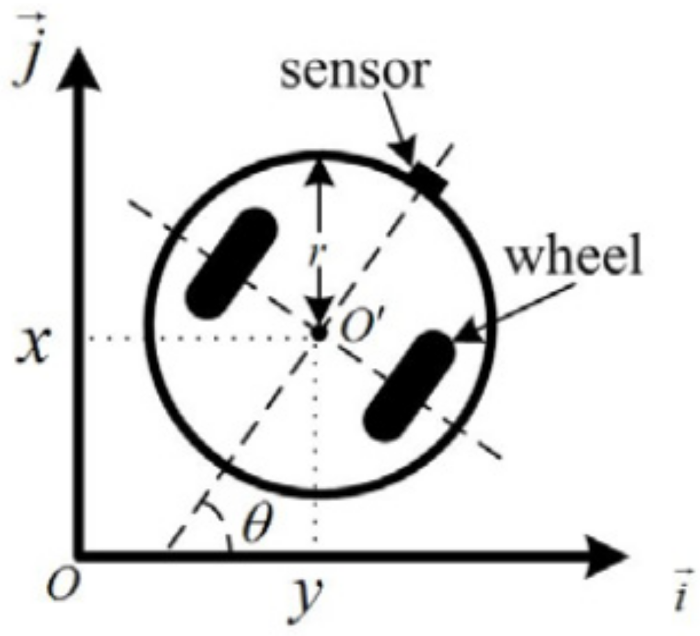
2.1. Model of a Robot

Figure 1 shows a unicycle-like robot in the horizontal plane. The diameter of this robot is 2r. Its two parallel wheels have the same axis and are controlled by two direct current motors independently. The robot can simultaneously rotate and translate, described by

$$q={\left[\begin{array}{ccc}x& y& \theta \end{array}\right]}^T$$

(1)

In (1), (x, y) is located at the center of the robot and represents its translational coordinates, and θ indicates its rotational coordinate. To know the position, a positioning sensor at the front castor of this robot is set up in Figure 1. The axis of the sensor is orthogonal to the axis of the two wheels.

On the assumption of pure rolling and no-slipping, the ideal kinematic model of this robot [3,4] has the form of

$$\dot{q}=\left[\begin{array}{c}\dot{x}\\ \dot{y}\\ \dot{\theta }\end{array}\right]=\left[\begin{array}{c}\begin{array}{cc}\cos \theta & 0\end{array}\\ \begin{array}{cc}\sin \theta & 0\end{array}\\ \begin{array}{cc}0& 1\end{array}\end{array}\right]\cdot \left[\begin{array}{c}v\\ \omega \end{array}\right]$$

(2)

$$\mathrm{s}. \mathrm{t}. \dot{x}\sin \theta -\dot{y}\cos \theta =0$$

(3)

Here, $v$ is the robot’s linear velocity in the X-Y coordinates and $\omega$ represents the angular velocity. The directions of the two vectors are that $v$ is positive when the robot moves in the positive direction of the X axis and that $\omega$ is positive when the robot rotates counterclockwise.

Concerning the constraint (3), the time derivative of (2), namely the ideal dynamic model, can be written as

$$\left[\begin{array}{c}\ddot{x}\\ \ddot{y}\\ \ddot{\theta }\end{array}\right]=\left[\begin{array}{c}-\dot{y}\dot{\theta }\\ \dot{x}\dot{\theta }\\ 0\end{array}\right]+\left[\begin{array}{c}\begin{array}{cc}\cos \theta & 0\end{array}\\ \begin{array}{cc}\sin \theta & 0\end{array}\\ \begin{array}{cc}0& 1\end{array}\end{array}\right]\cdot u$$

(4)

In (4), $u={[\begin{array}{cc}\dot{v}& \dot{\omega }\end{array}]}^T$. Here, $\dot{v}$ and $\dot{\omega }$ represent the acceleration and angular acceleration of the robot, respectively.

Since the robot in reality suffers from a variety of disturbances and uncertainties, for example, friction, slip, slide shift, etc., the real dynamic model [6] can be derived from (4).

$$\left[\begin{array}{c}\ddot{x}\\ \ddot{y}\\ \ddot{\theta }\end{array}\right]=\left[\begin{array}{c}-\dot{y}\dot{\theta }\\ \dot{x}\dot{\theta }\\ 0\end{array}\right]+\left[\begin{array}{c}\begin{array}{cc}\cos \theta & 0\end{array}\\ \begin{array}{cc}\sin \theta & 0\end{array}\\ \begin{array}{cc}0& 1\end{array}\end{array}\right]\cdot (u+\Delta \cdot u)+\pi \left(q,\dot{q}\right)$$

(5)

In (5), $\pi \left(q,\dot{q}\right)$ represents the lumped uncertainties and disturbances, defined by

$$\pi \left(q,\dot{q}\right)={[\begin{array}{ccc}{\pi }_x& {\pi }_y& {\pi }_{\theta }\end{array}]}^T$$

Here, ${\pi }_x$, ${\pi }_y$, and ${\pi }_{\theta }$ are the functions of the vectors $q$ and $\dot{q}$. $\Delta$ indicates the physical parameter changes of this robot, described by

$$\Delta =\left[\begin{array}{cc}\epsilon & 0\\ 0& {\epsilon }^{\prime }\end{array}\right]$$

Here, $\epsilon$ and ${\epsilon }^{\prime }$ are the changes of the mass and the inertia of the robot, respectively.

2.2. Model of a Leader-Follower Formation Pair

Consider a multi-robot system composed of N robots. Each robot is the same as the robot in Figure 1, where the robot i is assigned as the leader and takes charge of other robots, that is, there exist N−1 leader-follower pairs in this multi-robot system. Figure 2 illustrates a leader-follower pair made of the leader i and its follower k [27].

Some symbols in Figure 2 are represented as follows. For each individual robot, the subscripts i and k are adopted to describe the individual variables of the leader and the follower, respectively. The subscript ik is employed to depict the relative variables of the pair. Here, the relative distance l_ik means the distance between the leader’s center and the follower’s front castor, formulated by

$$l_{ik}=\sqrt{{\left(x_i-{\overline{x}}_k\right)}^2+{\left(y_i-{\overline{y}}_k\right)}^2}$$

(6)

Here,

$$\begin{array}{l}{\overline{x}}_k=x_k+r\cos {\theta }_k\\ {\overline{y}}_k=y_k+r\sin {\theta }_k\end{array}$$

The relative bearing angle ${\psi }_{ik}$ of the leader-follower pair is determined by

$${\psi }_{ik}=\pi +{\zeta }_{ik}-{\theta }_i$$

(7)

Here,

$${\zeta }_{ik}=\arctan \frac{y_i-y_k-r\sin {\theta }_k}{x_i-x_k-r\cos {\theta }_k}$$

The purpose of the paper was to investigate an adaptive-gain super-twisting sliding mode control design for formation maneuvers of this multi-robot system. Motivated by this purpose, the formation objective of the leader-follower scheme was that each leader-follower pair of the multi-robot system has to keep the desired relative distance and the desired relative bearing angle in spite of uncertainties and disturbances. In order to focus on the objective, some ideal conditions were taken in the multi-robot system: (1) There are neither collisions nor communication delay; (2) the follower is well-known, that is, it knows its position and velocity, meanwhile, it can obtain the position and velocity of the leader as well.

Define a vector x_ik = [x₁ x₂ x₃ x₄]^T. Let $x_1=l_{ik}$, $x_2={\dot{l}}_{ik}$, $x_3={\psi }_{ik}$ and $x_4={\dot{\psi }}_{ik}$. According to the formation objective, the relative distance $l_{ik}$ and the relative bearing angle ${\psi }_{ik}$ are determined as the formation control output. Then, the dynamics of formation maneuvers of the multi-robot system can have the form of (8) in light of the leader-follower scheme [14].

$$\begin{array}{l}{\dot{x}}_{ik}=f\left(x_{ik},d_{ik}\right)+g\left(x_{ik},{\Delta }_k\right)u_k\\ y_{ik}=h\left(x_{ik}\right)\end{array}$$

(8)

Here, x_ik is the system state vector and y_ik is the system output vector. Further,

$$\begin{array}{c}f\left(x_{ik},d_{ik}\right)=A_{ik}{x}_{ik}+B_{ik,2}{d}_{ik}\\ g\left(x_{ik},{\Delta }_k\right)=B_{ik,1}+B_{ik,1}{\Delta }_k\end{array}$$

A_ik,B_ik,1,B_ik,2, and h(x_ik) are depicted by

$$A_{ik}=\left[\begin{array}{cccc}0& 1& 0& 0\\ 0& 0& 0& 0\\ 0& 0& 0& 1\\ 0& 0& 0& 0\end{array}\right], B_{ik,2}=\left[\begin{array}{c}\begin{array}{cc}0& 0\end{array}\\ \begin{array}{cc}1& 0\end{array}\\ \begin{array}{cc}0& 0\end{array}\\ \begin{array}{cc}0& 1\end{array}\end{array}\right], B_{ik,1}=\left[\begin{array}{c}\begin{array}{cc}0& 0\end{array}\\ \begin{array}{cc}\cos {\phi }_{ik}& r\sin {\phi }_{ik}\end{array}\\ \begin{array}{cc}0& 0\end{array}\\ \begin{array}{cc}\frac{-\sin {\phi }_{ik}}{l_{ik}}& \frac{r\cos {\phi }_{ik}}{l_{ik}}\end{array}\end{array}\right], h\left(x_{ik}\right)=\left[\begin{array}{c}{x}_1\\ x_3\end{array}\right]$$

where ${\phi }_{ik}={\psi }_{ik}+{\theta }_{ik}$. $d_{ik}$ is the lumped term of all the uncertainties and disturbances in the leader-follower pair.

$$d_{ik}=L_{ik}\left(I_2+{\Delta }_i\right)u_i+F_{ik}+P_{ik}$$

(9)

In (9),

$$L_{ik}=\left[\begin{array}{cc}0& 0\\ -\cos {\psi }_{ik}& 0\\ 0& 0\\ \frac{\sin {\psi }_{ik}}{l_{ik}}& -1\end{array}\right], F_{ik}=\left[\begin{array}{c}0\\ F_1\\ 0\\ F_2\end{array}\right], P_{ik}=\left[\begin{array}{c}0\\ P_1\\ 0\\ P_2\end{array}\right]$$

Here, $I_2$ is a 2 × 2 identity matrix and F₁, F₂, P₁, and P₂ are written by

$$\begin{array}{cc}{F}_1=& ({\dot{\psi }}_{ik}{)}^2{l}_{ik}+2{\dot{\psi }}_{ik}{\dot{\theta }}_i{l}_{ik}+({\dot{\theta }}_i{)}^2{l}_{ik}\\ & -r\cos {\phi }_{ik}({\dot{\theta }}_k{)}^2-({\dot{y}}_k{\dot{\theta }}_k-{\dot{y}}_i{\dot{\theta }}_i)\cos ({\psi }_{ik}+{\dot{\theta }}_i)-({\dot{x}}_i{\dot{\theta }}_i-{\dot{x}}_k{\dot{\theta }}_k)\sin ({\psi }_{ik}+{\theta }_i)\\ F_2=& \frac{-({\dot{y}}_k{\dot{\phi }}_{ik}-{\dot{\psi }}_{ik}{\dot{y}}_i)\sin ({\psi }_{ik}+{\theta }_i)-r{\dot{\theta }}_k{\dot{\phi }}_{ik}\sin {\phi }_{ik}}{l_{ik}}\\ & \frac{-({\dot{x}}_k{\dot{\phi }}_{ik}-{\dot{\psi }}_{ik}{\dot{x}}_i)\cos ({\psi }_{ik}+{\theta }_i)+i_{ik}(({\dot{y}}_i-{\dot{y}}_k)\cos ({\psi }_{ik}+{\theta }_i)-({\dot{x}}_i-{\dot{x}}_k)\sin ({\psi }_{ik}+{\theta }_{{}_i})-r{\dot{\theta }}_k{\dot{\phi }}_{ik}\cos {\phi }_{ik})}{l_{ik}}\\ & P_1=-({\pi }_{ix}-{\pi }_{kx})\cos ({\psi }_{ik}+{\theta }_i)-({\pi }_{iy}-{\pi }_{ky})sin({\psi }_{ik}+{\theta }_i)+r{\pi }_{k\theta }\sin {\phi }_{ik}\\ & P_2=\frac{({\pi }_{ix}-{\pi }_{kx})sin({\psi }_{ik}+{\theta }_i)-({\pi }_{iy}-{\pi }_{ky})\cos ({\psi }_{ik}+{\theta }_i)+r{\pi }_{k\theta }\sin {\phi }_{ik}-l_{ik}{\pi }_{i\theta }}{l_{ik}}\end{array}$$

3. Control Design

3.1. Sliding Mode Design and Its Input-Output Dynamics

The super-twisting law is a powerful second-order sliding-mode technique [28]. It can effectively deal with the controlled plant with a relative degree equal to one with respect to the control input. Theoretically, the technique can make the sliding mode variable and its time derivative convergent to the origin in spite of the uncertainties and disturbances. Thus, this technique can be considered as a solution for formation maneuvers of the multi-robot system.

In order to implement the control design of the leader-follower pair, the sliding mode vector $s_{ik}$, that is, the sliding surfaces, has to be defined in advance.

$$s_{ik}=\left[\begin{array}{c}{s}_{ik,1}\\ s_{ik,2}\end{array}\right]=C_1\left(\left[\begin{array}{c}{l}_{ik}\\ {\psi }_{ik}\end{array}\right]-\left[\begin{array}{c}{l}_{ik}^d\\ {\psi }_{ik}^d\end{array}\right]\right)+C_2\left(\left[\begin{array}{c}{\dot{l}}_{ik}\\ {\dot{\psi }}_{ik}\end{array}\right]-\left[\begin{array}{c}{\dot{l}}_{ik}^d\\ {\dot{\psi }}_{ik}^d\end{array}\right]\right)$$

(10)

Here, $C_1$ and $C_2$ are 2 × 2 constant matrices and they need to be pre-defined. $l_{ik}^d$ and ${\psi }_{ik}^d$ are the desired relative distance and the desired relative bearing angle of this leader-follower pair, respectively.

Differentiate the sliding mode vector $s_{ik}$ in (10) with the respect to time, the input–output dynamics can be derived as follows.

$${\dot{s}}_{ik}=\frac{\partial s_{ik}}{\partial t}+\frac{\partial s_{ik}}{\partial x_{ik}}f\left(x_{ik},d_{ik}\right)+\frac{\partial s_{ik}}{\partial x_{ik}}g\left(x_{ik},{\Delta }_k\right)u_k$$

(11)

In (10) and (11), we have

$$\frac{\partial s_{ik}}{\partial u_k}=0 \mathrm{and} \frac{\partial {\dot{s}}_{ik}}{\partial u_k}=\frac{\partial s_{ik}}{\partial x_{ik}}g\left(x_{ik},{\Delta }_k\right)\ne 0$$

Namely, the relative degree of $s_{ik}$ with respect to $u_k$ is equal to 1. Subsequently, the super-twisting-based sliding mode control design can be available for formation maneuvers of such a multi-robot system.

Let

$$\begin{array}{l}a(x_{ik},d_{ik},t)=\frac{\partial s_{ik}}{\partial t}+\frac{\partial s_{ik}}{\partial x_{ik}}f\left(x_{ik},d_{ik}\right)\\ b(x_{ik},{\Delta }_k,t)=\frac{\partial s_{ik}}{\partial x_{ik}}g\left(x_{ik},{\Delta }_k\right)\end{array}$$

(12)

Assumption 1. 

$b(x_{ik},{\Delta }_k,t)$is a 2 × 2 matrix and contains both known and unknown parts, written by (13).

$$b(x_{ik},{\Delta }_k,t)=b_0(x_{ik},t)+\Delta b(x_{ik},{\Delta }_k,t)$$

(13)

Here $b_0(x_{ik},t)$ is a known positively definite matrix, $\Delta b_0(x_{ik},{\Delta }_k,t)$ is bounded but unknown, and the two parts of $b(x_{ik},{\Delta }_k,t)$ satisfy

$$||\Delta b(x_{ik},{\Delta }_k,t)b_0^{-1}(x_{ik},t)|{|}_2\le \gamma \left(x_{ik},t\right)<{\gamma }_1<1$$

(14)

where ${\gamma }_1$ is a unknown constant.

Assumption 2. 

$a(x_{ik},d_{ik},t)$is a 2 × 1 vector and contains both known and unknown parts, depicted by (15).

$$a(x_{ik},d_{ik},t)=a_1(x_{ik},t)+a_2(x_{ik},d_{ik},t)$$

(15)

Here, both $a_1(x_{ik},t)$ and $a_2(x_{ik},d_{ik},t)$ are bounded, and they satisfy

$$\begin{array}{l}||a_1(x_{ik},t)|{|}_{\infty }\le {\delta }_1\sqrt{||s_{ik}|{|}_2}\\ ||{\dot{a}}_2(x_{ik},d_{ik},t)|{|}_{\infty }\le {\delta }_2\end{array}$$

(16)

where ${\delta }_1$ and ${\delta }_2$ are positive but unknown.

Concerning Assumptions 1 and 2, the input-output dynamics of the sliding mode vector $s_{ik}$ in (11) can have the form of

$${\dot{s}}_{ik}=a(x_{ik},d_{ik},t)+b_1(x_{ik},{\Delta }_k,t){\varpi }_k$$

(17)

Here, $b_1(x_{ik},{\Delta }_k,t)=I_2+\Delta b(x_{ik},{\Delta }_k,t)b_0^{-1}(x_{ik},t)$ is a 2 × 2 matrix and ${\varpi }_k=b_0(x_{ik},t)u_k$.

From Assumption 1, we have

$$1-{\gamma }_1\le ||b_1(x_{ik},{\Delta }_k,t)|{|}_2\le 1+{\gamma }_1$$

3.2. Adaptive-Gain Super-Twisting Sliding Mode Design

According to the super-twisting law, the following sliding mode formation control approach was addressed. Considering the input-output dynamics (17), here the variable ${\varpi }_k$ is related to the control input $u_k$ so that their control design is equivalent to each other. Therefore, the following sliding mode control is formulated.

$${\varpi }_k={\varpi }_{k1}+{\varpi }_{k2}$$

(18)

Here,

$$\begin{array}{c}{\varpi }_{k1}=-{\alpha }_k\sqrt{||s_{ik}|{|}_2}\mathrm{sgn}(s_{ik})\\ {\dot{\varpi }}_{k2}=-\frac{{\beta }_k}{2}\mathrm{sgn}(s_{ik})\end{array}$$

where ${\alpha }_k$ and ${\beta }_k$ are the adaptive gains to be deduced from the closed-loop system stability. The signum function $\mathrm{sgn}(s_{ik})$ in (18) is determined by $\mathrm{sgn}(s_{ik})={\left[\begin{array}{cc}\mathrm{sgn}(s_{ik,1})& \mathrm{sgn}(s_{ik,2})\end{array}\right]}^T$.

From (17) and (18), the input-output dynamics can be re-written as

$$\begin{array}{l}{\dot{s}}_{ik}=-{\alpha }_k\sqrt{||s_{ik}|{|}_2}{b}_1\mathrm{sgn}(s_{ik})+a_1+{\varpi }_{k*}\\ {\dot{\varpi }}_{k*}=-\frac{{\beta }_k}{2}{b}_1\mathrm{sgn}(s_{ik})+{\dot{a}}_2+{\dot{b}}_1{\varpi }_{k2}\\ {\varpi }_{k*}(0)=0\end{array}$$

(19)

Here, $a_1(x_{ik},t)$, ${\dot{a}}_2(x_{ik},d_{ik},t)$, and ${\dot{b}}_1(x_{ik},{\Delta }_k,t)$ are abbreviated by $a_1$, ${\dot{a}}_2$, and ${\dot{b}}_1$ for brevity, and ${\varpi }_{k*}=a_2+b_1{\varpi }_{k2}$.

Assumption 3. 

${\dot{b}}_1{\varpi }_{k2}$in (19) is bounded but its boundary is unknown, that is,

$$||{\dot{b}}_1{\varpi }_{k2}|{|}_{\infty }\le {\delta }_3$$

(20)

Here, ${\delta }_3$is positive but unknown.

Substituting ${\varpi }_{k2}$ in (18) into (20) yields

$$||{\dot{b}}_1{\varpi }_{k2}|{|}_{\infty }\le \frac{||{\dot{b}}_1|{|}_{\infty }}{2}{\displaystyle {\int }_0^t{\beta }_k\mathrm{d}t}\le {\delta }_3$$

This fact indicates the adaptive gain ${\beta }_k$ is bounded as well, i.e.,

$$|{\beta }_k|\le {\beta }^{*}$$

(21)

Here, ${\beta }^{*}$ is positive but unknown.

Assumption 4. 

The adaptive gain${\alpha }_k$is bounded, that is,

$$|{\alpha }_k|\le {\alpha }^{*}$$

(22)

Here,${\alpha }^{*}$is positive but unknown.

Note that the uncertainties and disturbances of the input-output dynamics (17) exist in the terms $a_2$ and $b_1$. From Assumptions 2 and 3, the lumped boundary of the uncertain terms in (17) can be deduced from (16) and (22).

$$||\dot{\chi }|{|}_{\infty }=||{\dot{a}}_2+{\dot{b}}_1{\varpi }_{k2}|{|}_{\infty }\le ||{\dot{a}}_2|{|}_{\infty }+||{\dot{b}}_1{\varpi }_{k2}|{|}_{\infty }\le {\delta }_2+{\delta }_3={\delta }_4$$

(23)

where $\dot{\chi }={\dot{a}}_2+{\dot{b}}_1{\varpi }_{k2}$.

Until now, the formation control design has been equivalent to the deduction of the adaptive-gain laws in (18) that can make $s_{ik}$ and ${\dot{s}}_{ik}$ convergent to zero in finite time despite the uncertainties and disturbances, where the input-output dynamics are decided by (19) and the unknown boundaries ${\delta }_1$, ${\gamma }_1$, and ${\delta }_4$ are given by (14), (16), and (23). Finally, the adaptive gains are designed by

$$\begin{array}{c}{\dot{\alpha }}_k=\left\{\begin{array}{cc}\xi \sqrt{\frac{{\gamma }_1}{2}}\mathrm{sgn}(||s_{ik}|{|}_2-\mu )& \mathrm{if} {\alpha }_k>{\alpha }_m\\ \eta & \mathrm{if} {\alpha }_k<{\alpha }_m\end{array}\right.\\ {\beta }_k=2\epsilon {\alpha }_k\hfill & \end{array}$$

(24)

Here, ${\gamma }_1$ is determined by (14); $\epsilon$, $\xi$ and $\eta$ are arbitrary positive constants; ${\alpha }_m>0$ is an arbitrary small constant and the initial condition of ${\alpha }_k$ at t = 0 satisfies ${\alpha }_k(0)>{\alpha }_m$.

3.3. Stability Analysis of the Closed-Loop Control System

Theorem 1. 

Consider the dynamics (19), where$a_1$, $a_2$and$b_1$satisfy Assumptions 1 and 2 with the unknown gains${\delta }_1$, ${\delta }_2$, and${\gamma }_1$. The adaptive gains satisfy Assumptions 3 and 4 and they are determined by (24). Then, for any$x_{ik}$at t = 0, there exist

• a parameter$\mu >0$so that${\alpha }_k$satisfies (25) if$||s_{ik}|{|}_2>\mu$at t = 0;

  $${\alpha }_k>\frac{{\delta }_1(\lambda +4{\epsilon }^2)-\epsilon (4{\delta }_4+1)}{\lambda (1-{\gamma }_1)}+\frac{{[2\epsilon {\delta }_1-2{\delta }_4-\lambda -4{\epsilon }^2]}^2}{12\epsilon \lambda (1-{\gamma }_1)}$$

  (25)
  Here$\lambda$is an arbitrary positive constant and${\delta }_4$ is determined by (23).
• a finite time$t_F>0$so that the sliding modes of$s_{ik}$are reached in the finite time$t_F$regarding to the adaptive-gain super-twisting sliding mode control method, that is,$\forall t>t_F$, $\exists$$||s_{ik}|{|}_2\le {\eta }_1$and$||{\dot{s}}_{ik}|{|}_2\le {\eta }_2$. Here,${\eta }_1>\mu$and${\eta }_2>0$.
• both${\alpha }_k$and${\beta }_k$are bounded.

Proof. 

Preparation.

Define a 4 × 1 augmented vector $Z$

$$Z={\left[\begin{array}{cc}{Z}_1^T& Z_2^T\end{array}\right]}^T={\left[\begin{array}{cc}\sqrt{||s_{ik}|{|}_2}{[\mathrm{sgn}(s_{ik})]}^T& {[{\varpi }_{k*}]}^T\end{array}\right]}^T$$

(26)

Here, $||Z_1|{|}_{\infty }=\sqrt{||s_{ik}|{|}_2}$, $\mathrm{sgn}(Z_1)=\mathrm{sgn}(s_{ik})$ and $Z_2={\varpi }_{k*}$. Further, the time derivative of $Z_1$ and $Z_2$ can be written as

$$\begin{array}{l}{\dot{Z}}_1=\frac{1}{2}\frac{1}{||Z_1|{|}_{\infty }}\left[-{\alpha }_k{b}_1{Z}_1+Z_2+a_1\right]\\ {\dot{Z}}_2=-\frac{{\beta }_k}{2}{b}_1\frac{Z_1}{||Z_1|{|}_{\infty }}+\dot{\chi }\end{array}$$

(27)

From (27), we have

$$\left[\begin{array}{c}{\dot{Z}}_1\\ {\dot{Z}}_2\end{array}\right]=\frac{1}{2||Z_1|{|}_{\infty }}\left[\begin{array}{cc}-{\alpha }_k{b}_1& I_2\\ -{\beta }_k{b}_1& O_2\end{array}\right]\left[\begin{array}{c}{Z}_1\\ Z_2\end{array}\right]+\frac{1}{2||Z_1|{|}_{\infty }}\left[\begin{array}{c}{a}_1\\ 2||Z_1|{|}_{\infty }\dot{\chi }\end{array}\right]$$

(28)

Here, $O_2$ is a 2 × 2 zero matrix.

Further, considering (16) and (23), two bounded scalar functions ${\rho }_1(x_{ik},t)$ and ${\rho }_2(x_{ik},t)$ can be constructed as

$$\begin{array}{l}{a}_1={\rho }_1(x_{ik},t)\sqrt{||s_{ik}|{|}_2}\mathrm{sgn}(s_{ik})={\rho }_1(x_{ik},t)Z_1\\ \dot{\chi }=\frac{{\rho }_2(x_{ik},t)}{2}\frac{\sqrt{||s_{ik}|{|}_2}}{\sqrt{||s_{ik}|{|}_2}}\mathrm{sgn}(s_{ik})=\frac{{\rho }_2(x_{ik},t)}{2}\frac{Z_1}{||Z_1|{|}_{\infty }}\end{array}$$

(29)

Then, we can have

$$\begin{array}{l}0<{\rho }_1(x_{ik},t)<{\delta }_1\\ 0<{\rho }_2(x_{ik},t)<2{\delta }_4\end{array}$$

(30)

Substituting (29) into (28) yields

$$\left[\begin{array}{c}{\dot{Z}}_1\\ {\dot{Z}}_2\end{array}\right]=\overline{A}\left[\begin{array}{c}{Z}_1\\ Z_2\end{array}\right]$$

(31)

Here, $\overline{A}=\frac{1}{2||Z_1|{|}_{\infty }}\left[\begin{array}{cc}-{\alpha }_k{b}_1+{\rho }_1(x_{ik},t)I_2& I_2\\ -{\beta }_k{b}_1+{\rho }_2(x_{ik},t)I_2& O_2\end{array}\right]$.

Consider a Lyapunov candidate as

$$V_0=Z^{T}PZ$$

(32)

Here, $P=\left[\begin{array}{cc}(\lambda +4{\epsilon }^2)I_2& -2\epsilon I_2\\ -2\epsilon I_2& I_2\end{array}\right]$ is a 4 × 4 positive definite matrix, $\lambda >0$ and $\epsilon >0$.

From (31), the time derivative of $V_0$ in (32) can be written by

$${\dot{V}}_0={\dot{Z}}^{T}PZ+Z^{T}P\dot{Z}=Z^T\left({\overline{A}}^{T}P+P{\overline{A}}^T\right)Z\le -\frac{1}{2||Z_1|{|}_{\infty }}{Z}^T\overline{Q}Z$$

(33)

Here, $\overline{Q}=\left[\begin{array}{cc}{\overline{Q}}_{11}& {\overline{Q}}_{12}\\ {\overline{Q}}_{21}& 4\epsilon \end{array}\right]$ is a 4 × 4 symmetric matrix, ${\overline{Q}}_{11}$, ${\overline{Q}}_{12}$ and ${\overline{Q}}_{21}$ are given by

$${\overline{Q}}_{11}=2\lambda {\alpha }_k{b}_1+4\epsilon (2\epsilon {\alpha }_k-{\beta }_k)b_1-[2(\lambda +4{\epsilon }^2){\rho }_1(x_{ik},t)-4\epsilon {\rho }_2(x_{ik},t)]I_2$$

$${\overline{Q}}_{12}={\overline{Q}}_{21}=({\beta }_k-2\epsilon {\alpha }_k)b_1+[2\epsilon {\rho }_1(x_{ik},t)-{\rho }_2(x_{ik},t)]I_2-(\lambda +4{\epsilon }^2)I_2$$

From the aspect of the stability of $V_0$, $\overline{Q}$ is not only symmetric but also positive definite in the sense of Lyapunov. Therefore, we selected ${\beta }_k=2\epsilon {\alpha }_k$ in ${\overline{Q}}_{11}$. Then, $\overline{Q}$ can be positive definite and its minimal eigenvalue is ${\lambda }_{\min }(\overline{Q})\ge 2\epsilon$ if ${\alpha }_k$ satisfies (25).

From (32), we have

$${\lambda }_{\min }(P)||Z|{|}_2^2\le Z^{T}PZ=V_0\le {\lambda }_{\max }(P)||Z|{|}_2^2$$

(34)

Further, (35) can be deduced from (33) if (25) holds true.

$${\dot{V}}_0\le -\frac{1}{2||Z_1|{|}_{\infty }}{Z}^T\overline{Q}Z\le -\frac{2\epsilon }{2||Z_1|{|}_{\infty }}{Z}^{T}Z=-\frac{\epsilon ||Z|{|}_2^2}{||Z_1|{|}_{\infty }}$$

(35)

In (26), the following inequality exists.

$$||Z_1|{|}_{\infty }=\sqrt{||s_{ik}|{|}_2}\le ||Z_1|{|}_2\le ||Z|{|}_2\le {\left(\frac{V_0}{{\lambda }_{\min }(P)}\right)}^{1/2}$$

(36)

With regard to (34) and (36), (35) can be re-written by

$${\dot{V}}_0\le -\frac{\epsilon {\lambda }_{\min }^{1/2}(P)}{{\lambda }_{\max }(P)}{V}_0^{1/2}$$

(37)

Analysis.

Now, the closed-looped control system stability will be presented in the sense of Lyapunov. Define a Lyapunov candidate as

$$V=V_0+\frac{1}{2{\gamma }_1}{({\alpha }_k-{\alpha }^{*})}^2+\frac{1}{2{\gamma }_2}{({\beta }_k-{\beta }^{*})}^2$$

(38)

Here, ${\alpha }^{*}$ and ${\beta }^{*}$ are given in Assumptions 3 and 4. Concerning (33) and (37), the time derivative of $V$ can have the form of

$$\dot{V}={\dot{V}}_0+\frac{1}{{\gamma }_1}({\alpha }_k-{\alpha }^{*})\dot{\alpha }+\frac{1}{{\gamma }_2}({\beta }_k-{\beta }^{*})\dot{\beta }$$

(39)

From (37), (39) can be written as

$$\begin{array}{ll}\dot{V}& \le -\frac{\epsilon {\lambda }_{\min }^{1/2}(P)}{{\lambda }_{\max }(P)}{V}_{{}_0}^{1/2}+\frac{1}{{\gamma }_1}{\epsilon }_{\alpha }{\dot{\alpha }}_k+\frac{1}{{\gamma }_2}{\epsilon }_{\beta }{\dot{\beta }}_k\\ & =-\frac{\epsilon {\lambda }_{\min }^{1/2}(P)}{{\lambda }_{\max }(P)}{V}_{{}_0}^{1/2}-\frac{{\xi }_1}{\sqrt{2{\gamma }_1}}|{\epsilon }_{\alpha }|-\frac{{\xi }_2}{\sqrt{2{\gamma }_2}}|{\epsilon }_{\beta }|+\frac{1}{{\gamma }_1}{\epsilon }_a{\dot{\alpha }}_k+\frac{1}{{\gamma }_2}{\epsilon }_{\beta }{\dot{\beta }}_k+\frac{{\xi }_1}{\sqrt{2{\gamma }_1}}|{\epsilon }_{\alpha }|+\frac{{\xi }_2}{\sqrt{2{\gamma }_2}}|{\epsilon }_{\beta }|\end{array}$$

(40)

Here, ${\epsilon }_{\alpha }={\alpha }_k-{\alpha }^{*}$ and ${\epsilon }_{\beta }={\beta }_k-{\beta }^{*}$. It is apparent that both ${\epsilon }_{\alpha }$ and ${\epsilon }_{\beta }$ are negative or equal to zero according to Assumptions 3 and 4.

Since ${({\tilde{a}}^2+{\tilde{b}}^2+{\tilde{c}}^2)}^{\frac{1}{2}}\le |\tilde{a}|+|\tilde{b}|+|\tilde{c}|$, it is concluded that

$$-\frac{\epsilon {\lambda }_{\min }^{1/2}(P)}{{\lambda }_{\max }(P)}{V}_{{}_0}^{1/2}-\frac{{\xi }_1}{\sqrt{2{\gamma }_1}}|{\epsilon }_{\alpha }|-\frac{{\xi }_2}{\sqrt{2{\gamma }_2}}|{\epsilon }_{\beta }|\le -{\eta }_0{V}^{1/2}$$

Here, ${\eta }_0=\min (\frac{\epsilon {\lambda }_{\min }^{1/2}(P)}{{\lambda }_{\max }(P)}, {\xi }_1, {\xi }_2)$. Then, (40) can have the form of

$$\dot{V}\le -{\eta }_0{V}^{1/2}+\frac{1}{{\gamma }_1}{\epsilon }_{\alpha }{\dot{\alpha }}_k+\frac{1}{{\gamma }_2}{\epsilon }_{\beta }{\dot{\beta }}_k+\frac{{\xi }_1}{\sqrt{2{\gamma }_1}}|{\epsilon }_{\alpha }|+\frac{{\xi }_2}{\sqrt{2{\gamma }_2}}|{\epsilon }_{\beta }|$$

(41)

Since both ${\epsilon }_{\alpha }$ and ${\epsilon }_{\beta }$ in (41) are equal to or less than zero, we can obtain

$$\dot{V}\le -{\eta }_0{V}^{1/2}-|{\epsilon }_{\alpha }|(\frac{1}{{\gamma }_1}{\dot{\alpha }}_k-\frac{{\xi }_1}{\sqrt{2{\gamma }_1}})-|{\epsilon }_{\beta }|(\frac{1}{{\gamma }_2}{\dot{\beta }}_k-\frac{{\xi }_2}{\sqrt{2{\gamma }_2}})$$

(42)

The motivation of designing the adaptive gains is to investigate a domain. The domain acts as a flag. The gains ${\alpha }_k$ and ${\beta }_k$ can start dynamically reducing when the system trajectories come to the domain in finite time. Once the trajectories leave the domain, the gains start dynamically increasing in order to draw the trajectories back. Inspired by the methodology of sliding mode, we picked up the domain $||s_{ik}|{|}_2\le \mu$ as this flag. Thereafter, (42) is deduced by different cases in accordance with such a flag.

Case 1. 

$||s_{ik}|{|}_2>\mu$and${\alpha }_k>{\alpha }_m$for all$t\ge 0$. Take (24) into account. With regard to this case, (43) can be deduced from (24).

$${\dot{\alpha }}_k={\xi }_1\sqrt{\frac{{\gamma }_1}{2}}$$

(43)

Therefore, (42) becomes

$$\dot{V}\le -{\eta }_0{V}^{1/2}-|{\epsilon }_{\beta }|(\frac{1}{{\gamma }_2}{\dot{\beta }}_k-\frac{{\xi }_2}{\sqrt{2{\gamma }_2}})$$

(44)

Picking up $\epsilon =\frac{{\xi }_2}{2{\xi }_1}\sqrt{\frac{{\gamma }_2}{{\gamma }_1}}$ in (14) and substituting it into the time derivative of ${\beta }_k=2\epsilon {\alpha }_k$ yields

$${\dot{\beta }}_k={\xi }_2\sqrt{\frac{{\gamma }_2}{2}}$$

(45)

Finally, (44) becomes

$$\dot{V}\le -{\eta }_0{V}^{1/2}$$

(46)

Associated with the closed-loop system stability, (33) must be held true in order to have the positive definite matrix $\overline{Q}$, meaning that $\alpha$ should be increased as its adaptive law (24) until (33) is satisfied in the finite time $t_F$. From this time $t_F$ on, (46) will guarantee the convergence of this closed-loop system to the domain $||s_{ik}|{|}_2\le \mu$.

Case 2. 

$||s_{ik}|{|}_2\le \mu$. Take (24) into account. According to the motivation,${\alpha }_k$needs to be reduced in light of the adaptive law (24) so that it has a form of

$${\dot{\alpha }}_k=\left\{\begin{array}{cc}-\xi \sqrt{\frac{{\gamma }_1}{2}}& \mathrm{if} {\alpha }_k>{\alpha }_m\\ \eta & \mathrm{if} {\alpha }_k<{\alpha }_m\end{array}\right.$$

(47)

Meanwhile, picking up $\epsilon =\frac{{\xi }_2}{2{\xi }_1}\sqrt{\frac{{\gamma }_2}{{\gamma }_1}}$ in (14) and substituting it into the time derivative of ${\beta }_k=2\epsilon {\alpha }_k$ yields

$${\dot{\beta }}_k=\left\{\begin{array}{c}-{\xi }_2\sqrt{\frac{{\gamma }_2}{2}}\hspace{1em}\hspace{1em}\mathrm{if} {\alpha }_k>{\alpha }_m\\ \frac{{\xi }_2}{{\xi }_1}\sqrt{\frac{{\gamma }_2}{{\gamma }_1}}\eta \hspace{1em}\hspace{1em}\mathrm{if} {\alpha }_k<{\alpha }_m\end{array}\right.$$

(48)

Consequently, (42) becomes

$$\dot{V}\le \left\{\begin{array}{cc}-{\eta }_0{V}^{1/2}+2|{\epsilon }_{\alpha }|\frac{{\xi }_1}{\sqrt{2{\gamma }_1}}+2|{\epsilon }_{\beta }|\frac{{\xi }_2}{\sqrt{2{\gamma }_2}}\hfill & \mathrm{if} {\alpha }_k>{\alpha }_m\hfill \\ -{\eta }_0{V}^{1/2}-|{\epsilon }_{\alpha }|(\frac{\eta }{{\gamma }_1}-\frac{{\xi }_1}{\sqrt{2{\gamma }_1}})-|{\epsilon }_{\beta }|(\frac{{\xi }_2}{{\xi }_1}\frac{\eta }{\sqrt{{\gamma }_1{\gamma }_2}}-\frac{{\xi }_2}{\sqrt{2{\gamma }_2}})\hfill & \mathrm{if} {\alpha }_k<{\alpha }_m\hfill \end{array}\right.$$

(49)

Equation (49) indicates that the sign of the time derivative of $V$ is indefinite so that $||s_{ik}|{|}_2$ may become larger than $\mu$ with the decrease of ${\alpha }_k$ and ${\beta }_k$. Once $||s_{ik}|{|}_2$ becomes greater than $\mu$, the condition defined in Case 1 will be immediately triggered. In (46), the time derivative of $V$ is negative so that the closed-looped control system possesses the inherent stability and $s_{ik}$ will enter the domain $||s_{ik}|{|}_2<\mu$ again in finite time. This process continues back and forth until the control system becomes convergent. In this process, $s_{ik}$ may deviate from the domain for a finite time but there always exists another domain in the real sliding modes of $s_{ik}$.

$$||s_{ik}|{|}_2\le {\eta }_1\hspace{1em}({\eta }_1>\mu )$$

(50)

Inside the domain $||s_{ik}|{|}_2<\mu$, the value of $||{\dot{s}}_{ik}|{|}_2$ can estimated from (19) and (24).

$$||{\dot{s}}_{ik}|{|}_2\le \left[\left(1-{\gamma }_1\right){\alpha }_k(t_1)+{\delta }_1\right]{\mu }^{1/2}+\left[\epsilon (1-{\gamma }_1){\alpha }_k(t_1)+{\delta }_4\right]\left(t_2-t_1\right)={\overline{\eta }}_2$$

(51)

Here, t₁ is the time instant when $s_{ik}$ enters the domain $||s_{ik}|{|}_2\le \mu$ and t₂ is the moment when $s_{ik}$ leaves the domain. Once $||s_{ik}|{|}_2$ becomes $\mu <||s_{ik}|{|}_2<{\eta }_1$, we have

$$||{\dot{s}}_{ik}|{|}_2\le \left(1+{\gamma }_1\right)\left({\eta }_1{}^{1/2}+\epsilon \right)\left({\alpha }_k(t_2)+{\xi }_1\sqrt{\frac{{\eta }_1{\gamma }_1}{2}}+\epsilon \right)\left(t_3-t_2\right)+{\delta }_1{\eta }_1{}^{1/2}+{\delta }_4\left(t_3-t_2\right)={\tilde{\eta }}_2$$

(52)

Here, t₂ is the time instant when $s_{ik}$ leaves the domain $||s_{ik}|{|}_2<\mu$ and t₃ is the moment when $s_{ik}$ enter the domain $||s_{ik}|{|}_2<\mu$. Subsequently, (53) can be drawn from (51) and (52).

$$||{\dot{s}}_{ik}|{|}_2\le \max \left({\tilde{\eta }}_2, {\overline{\eta }}_2\right)={\eta }_2$$

(53)

From (50) and (52), there exist the real sliding modes, described by

$$\mathsf{\Omega }=\left\{\begin{array}{ccc}{s}_{ik},{\dot{s}}_{ik}:& ||s_{ik}|{|}_2\le {\eta }_1& ||{\dot{s}}_{ik}|{|}_2\le {\eta }_2\end{array}\hspace{1em}\hspace{1em}\hspace{1em}{\eta }_1>\mu \right\}$$

(54)

The existences of the sliding modes in (52) can be presented in theory, but ${\eta }_1$ and ${\eta }_2$ cannot be obtained in advance before a real control process is carried out.

Further, a solution of (24) in the domain $\mu <||s_{ik}|{|}_2\le {\eta }_1$ can be gotten as

$${\alpha }_k={\alpha }_k(0)+{\xi }_{1}t\sqrt{\frac{{\gamma }_1}{2}}\hspace{1em}\hspace{1em}\hspace{1em}0\le t\le t_F$$

(55)

Equation (54) indicates that the adaptive gain ${\alpha }_k$ is bounded so that the gain ${\beta }_k$ is bounded on account of ${\beta }_k=2\epsilon {\alpha }_k$. Inside the domain $||s_{ik}|{|}_2\le \mu$, the adaptive gains ${\alpha }_k$ and ${\beta }_k$ can be decreased as the presented control design. Consequently, ${\alpha }_k$ and ${\beta }_k$ are bounded.

Hitherto, the three pieces of results in Theorem 1 have been proven. In the next section, this presented control method will be carried out for the formation maneuvers of an uncertain multi-robot system made of such several leader-follower pairs. □

4. Implementation

4.1. Multi-Robot Simulation Platform

In order to demonstrate the feasibility of the designed formation control method, a multi-robot system platform was established in this section. The platform contains three identical robots shown in Figure 1, where the robot numbered by 1 is assigned as the leader and other two robots numbered by 2 and 3 become its followers. The number of this plat form is 3 so that the formation system is a typical small-scale one, indicating that some assumptions such as no collisions and no communication delay can easily be held true. The robot radius is set by r = 0.05 m. Considering this platform, the parameter $\Delta$ in (5) written as ${\Delta }_1$, ${\Delta }_2$ and ${\Delta }_3$ for the three robots has the form of

$${\Delta }_1={\Delta }_2={\Delta }_3=\left[\begin{array}{cc}\overline{\Delta }& 0\\ 0& \overline{\Delta }\end{array}\right]$$

(56)

Here, $\overline{\Delta }$ is set by 0.3 × rad−0.2 and rad is random between 0 and 1. Other parameters indicate the uncertainties and disturbances are formulated by

$$\begin{array}{c}{\pi }_{1x}={\pi }_{1y}={\pi }_{1\theta }=0.5\sin (2\pi t)\\ {\pi }_{2x}={\pi }_{2y}={\pi }_{2\theta }={\pi }_{3x}={\pi }_{3y}={\pi }_{3\theta }=0.3\sin (2\pi t)\end{array}$$

(57)

Concerning each follower, the parameters of their formation controller are set by $\epsilon =1$, ${\gamma }_1=2$, $\xi =2$, $\mu =0.7$, ${\alpha }_m=0.01$, and $\eta ={\alpha }_m$. Their parameters of the sliding modes are set by $C_1=\left[\begin{array}{cc}400& 0\\ 0& 400\end{array}\right]$ and $C_2=\left[\begin{array}{cc}56& 0\\ 0& 56\end{array}\right]$. Considering the adaptive gains of the two followers, the initial values of ${\alpha }_2$ and ${\alpha }_3$ is picked up as (19) and (21), respectively. Meanwhile, the initial value of the super-twisting law in (18) is given by ${\varpi }_{22}={\varpi }_{32}=2$.

4.2. Simulation Results

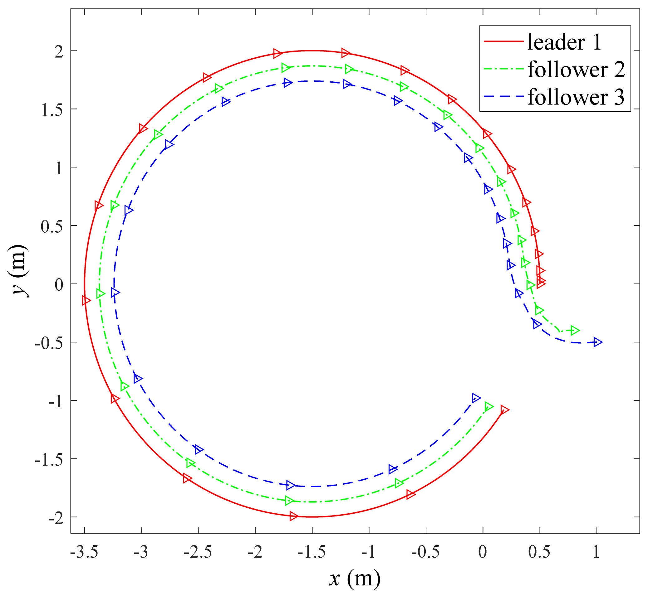
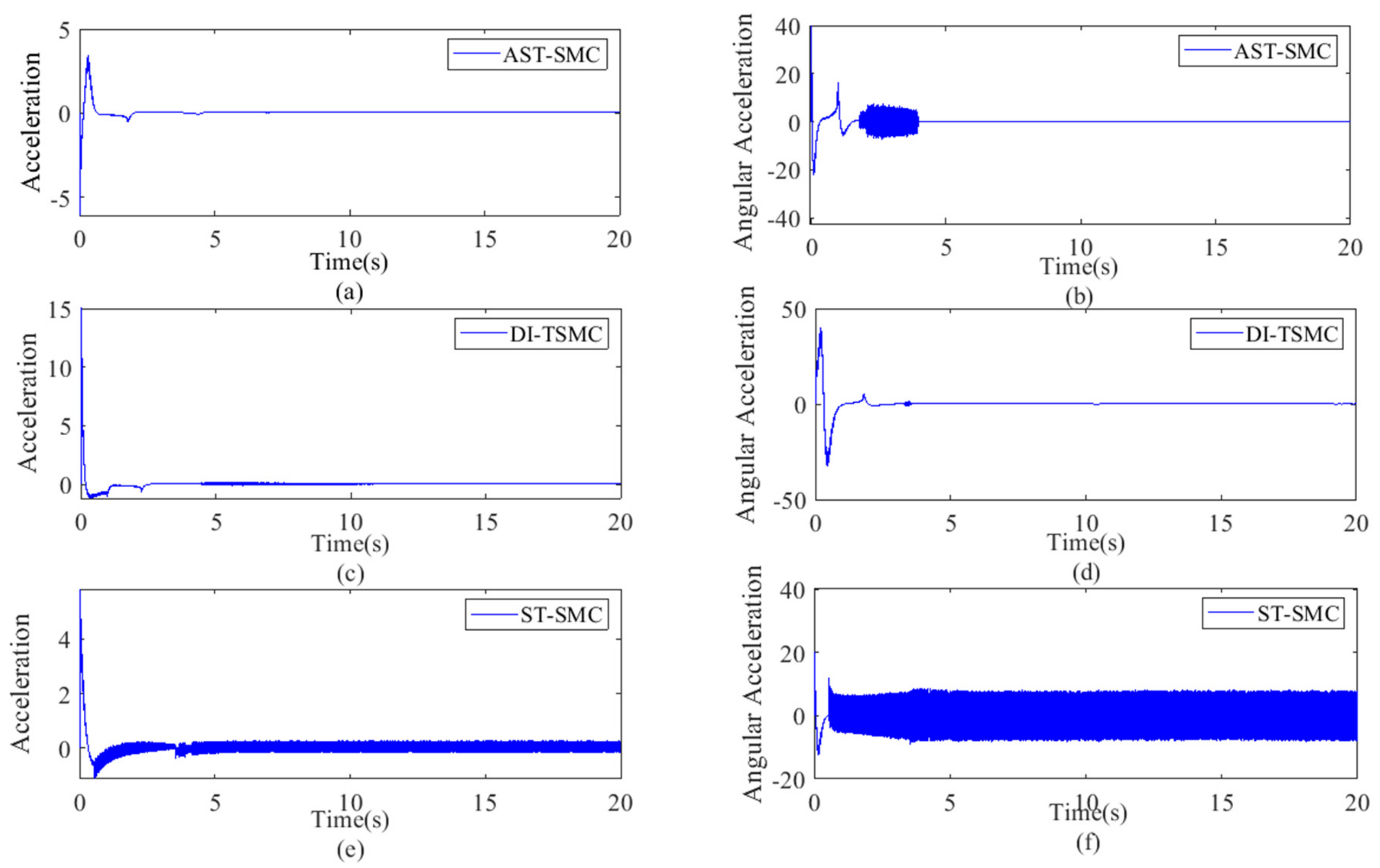
4.2.1. String Formation When Moving along a Circular Trajectory

In Figure 3, the multi-robot platform carries out the task of string formation when moving along a circular trajectory, where the red means the leader robot and the green and blue delegate the two followers. The initial postures of the three robots are allocated at

$$q_1=[{\begin{array}{ccc}0.5\mathrm{m}& 0\mathrm{m}& 0.5\pi \mathrm{rad}]\end{array}}^T, q_2={[\begin{array}{ccc}0.8\mathrm{m}& -0.4\mathrm{m}& 0\mathrm{rad}\end{array}]}^T, q_3=[{\begin{array}{ccc}1\mathrm{m}& -0.5\mathrm{m}& \pi \mathrm{rad}]\end{array}}^T$$

(58)

According to the initial postures and the formation task, the initial states of the formation dynamics (8) can be calculated as

$$x_{12}(0)={[\begin{array}{cccc}0.525\mathrm{m}& 0\mathrm{m}/\mathrm{s}& 0.8\pi \mathrm{rad}& 0\mathrm{rad}/\mathrm{s}\end{array}]}^T, x_{13}(0)={[\begin{array}{cccc}0.707\mathrm{m}& 0\mathrm{m}/\mathrm{s}& 0.75\pi \mathrm{rad}& 0\mathrm{rad}/\mathrm{s}\end{array}]}^T$$

(59)

Similarly, the desired states of the two followers are assigned by

$$x_{12}^d={[\begin{array}{cccc}0.13\mathrm{m}& 0\mathrm{m}/\mathrm{s}& 0.5\pi \mathrm{rad}& 0\mathrm{rad}/\mathrm{s}\end{array}]}^T, x_{13}^d={[\begin{array}{cccc}0.26\mathrm{m}& 0\mathrm{m}/\mathrm{s}& 0.5\pi \mathrm{rad}& 0\mathrm{rad}/\mathrm{s}\end{array}]}^T$$

(60)

The leader’s linear speed and its angular velocity are set as $v_1=0.5\mathrm{m}/\mathrm{s}$ and ${\omega }_1=1\mathrm{rad}/\mathrm{s}$.

Figure 4 demonstrates the state variables in (8) when the multi-robot system fulfills the formation task in Figure 3. For the purpose of comparisons, the other three classic control methods were also implemented on the same platform to accomplish the same formation task besides the presented control method (short for AST-SMC in Figure 4). These control methods are listed as the derivative-integral terminal sliding mode control [14] (short for DI-TSMC in Figure 4) and the sole super-twisting sliding mode control without any adaptive gains (short for ST-SMC in Figure 4).

From Figure 4, the presented control method can apparently improve the performance of the system state variables in (8). Note that the sole super-twisting sliding mode control is with the same sliding surfaces formulated by (10). From this aspect, the adaptive laws of the gains can benefit the improvement of the control performance. Furthermore, the control inputs of the three control methods applied to the follower 2 and the follower 3 are illustrated in Figure 5 and Figure 6, respectively.

Shown in Figure 5 and Figure 6, the adaptive-gain super-twisting sliding mode control method can decrease the chattering phenomenon effectively. In theory, the adaptive-gain super-twisting sliding mode control can completely compensate the disturbances and uncertainties entering the formation control system by the control channel. However, the formation dynamics (8) contain some disturbances and uncertainties that enter the control system by other channels. Therefore, the control inputs have to frequently switch to resist their adverse effects.

Figure 7 illustrate the sliding surfaces of the adaptive-gain super-twisting sliding mode control method. The gains ${\alpha }_2$, ${\beta }_2$, ${\alpha }_3$, and ${\beta }_3$ governed by the designed adaptive law (24) are demonstrated in Figure 8. As proven in Theorem 1, the sliding surfaces are convergent in infinite time although the time instants cannot be known in advance. Further, the curves of the gains in Figure 8 are not convergent. In fact, they are bounded as proven in Theorem 1.

4.2.2. String Formation When Moving along an S-Shape Trajectory

This platform in Figure 9 forms up a string when moving along an S-shape trajectory. Both the adaptive law and the controller parameters were kept unchanged. They are the same as the formation task in Figure 3. Concerning this task, the initial postures of the three robots are set by

$$q_1=[{\begin{array}{ccc}0.5\mathrm{m}& 0\mathrm{m}& 0\mathrm{rad}]\end{array}}^T, q_2={[\begin{array}{ccc}1.2\mathrm{m}& 0.5\mathrm{m}& 0\mathrm{rad}\end{array}]}^T, q_3=[{\begin{array}{ccc}2\mathrm{m}& 2\mathrm{m}& \pi \mathrm{rad}]\end{array}}^T$$

(61)

According to this control task and the initial postures, the initial states of the formation dynamics can be calculated by

$$x_{12}(0)={[\begin{array}{cccc}0.9\mathrm{m}& 0\mathrm{m}/\mathrm{s}& 1.8\pi \mathrm{rad}& 0\mathrm{rad}/\mathrm{s}\end{array}]}^T, x_{13}(0)={[\begin{array}{cccc}2.47\mathrm{m}& 0\mathrm{m}/\mathrm{s}& 0.3\pi \mathrm{rad}& 0\mathrm{rad}/\mathrm{s}\end{array}]}^T$$

(62)

Similarly, the desired states can be obtained by (59) on account of the leader’s trajectory.

$$x_{12}^d={[\begin{array}{cccc}0.9\mathrm{m}& 0\mathrm{m}/\mathrm{s}& 0.3\pi \mathrm{rad}& 0\mathrm{rad}/\mathrm{s}\end{array}]}^T, x_{13}^d={[\begin{array}{cccc}1.6\mathrm{m}& 0\mathrm{m}/\mathrm{s}& 0.7\pi \mathrm{rad}& 0\mathrm{rad}/\mathrm{s}\end{array}]}^T$$

(63)

The state variables and the control inputs are also similar to the formation task in Figure 3 as proven in Theorem 1 so that these curves are not be demonstrated, owing to the limited space.

4.2.3. String Formation When Moving Along a Straight Trajectory

This platform in Figure 10 forms up a string when moving along a straight trajectory. Both the adaptive law and the controller parameters were kept unchanged. The state variables and the control inputs are not illustrated because they are similar to Figure 3. The initial postures of the three robots are set by

$$q_1=[{\begin{array}{ccc}0.5\mathrm{m}& 0\mathrm{m}& \frac{1}{2}\pi \mathrm{rad}]\end{array}}^T, q_2={[\begin{array}{ccc}1.2\mathrm{m}& 0.5\mathrm{m}& 0\mathrm{rad}\end{array}]}^T, q_3=[{\begin{array}{ccc}2\mathrm{m}& 1\mathrm{m}& \pi \mathrm{rad}]\end{array}}^T$$

(64)

According to this control task and the initial postures, the initial states of the formation dynamics can be calculated by

$$x_{12}(0)={[\begin{array}{cccc}0.9\mathrm{m}& 0\mathrm{m}/\mathrm{s}& 1.69\pi \mathrm{rad}& 0\mathrm{rad}/\mathrm{s}\end{array}]}^T, x_{13}(0)={[\begin{array}{cccc}1.7\mathrm{m}& 0\mathrm{m}/\mathrm{s}& 1.65\pi \mathrm{rad}& 0\mathrm{rad}/\mathrm{s}\end{array}]}^T$$

(65)

Similarly, the desired states can be obtained by (59) on account of the leader’s trajectory.

$$x_{12}^d={[\begin{array}{cccc}0.3\mathrm{m}& 0\mathrm{m}/\mathrm{s}& 1.2\pi \mathrm{rad}& 0\mathrm{rad}/\mathrm{s}\end{array}]}^T, x_{13}^d={[\begin{array}{cccc}0.6\mathrm{m}& 0\mathrm{m}/\mathrm{s}& 1.8\pi \mathrm{rad}& 0\mathrm{rad}/\mathrm{s}\end{array}]}^T$$

(66)

The simulation results in Figure 9 and Figure 10 indicate that the presented control method is available for various formation patterns in spite of the adverse effects of uncertainties and disturbances. This fact means such an adaptive-gain super-twisting sliding mode control method is an alternative solution for the formation maneuvers of uncertain multi-robot systems under the mild assumption that the uncertainties and disturbances are bounded by an unknown boundary.

5. Conclusions

This paper concentrated on the formation control of multi-robot systems. In order to accomplish the formation task despite the inevitable disturbances and uncertainties, the super-twisting sliding mode control method was adopted. For the sake of dealing with the overestimate of the control gains, the adaptive laws of the gains were deduced. Theoretically, this adaptive-gain super-twisting sliding mode control method for the formation maneuvers was investigated in the sense of Lyapunov. Such a control method can guarantee the convergence of the sliding surfaces and make the adaptive gains bounded. Practically, the control method was applied to a multi-robot platform with three mobile robots. Some comparisons have been illustrated by the other two control methods, that is, the derivative-integral terminal sliding mode control and the sole super-twisting sliding mode control with no adaptive laws. The numerical results illustrate that the presented method has the best performance. The presented control method can be a solid support to solve the formation maneuvers of uncertain multi-robot systems.

References

1. Guillet, A.; Lenain, R.; Thuilot, B.; Martinet, P. Adaptable robot formation control: Adaptive and predictive formation control of autonomous vehicles. IEEE Robot Autom. Mag. 2014, 21, 28–39. [Google Scholar] [CrossRef]
2. Dai, Y.Y.; Qian, D.W.; Lee, S. Multiple robots motion control to transport an object. Filomat 2018, 32, 1547–1558. [Google Scholar] [CrossRef] [Green Version]
3. Dey, A.; Son, L.H.; Kumar, P.K.K.; Selvachandran, G.; Quek, S.G. New concepts on vertex and edge coloring of simple vague graphs. Symmetry 2018, 10, 373. [Google Scholar] [CrossRef]
4. Qian, D.W.; Tong, S.W.; Guo, J.R.; Lee, S.G. Leader-follower-based formation control of non-holonomic mobile robots with mismatched uncertainties via integral sliding mode. Proc. Inst. Mech. Eng. Part I J. Syst. Control Eng. 2015, 229, 559–569. [Google Scholar] [CrossRef]
5. Qian, D.W.; Tong, S.W.; Li, C.D. Observer-based leader-following formation control of uncertain multiple agents by integral sliding mode. Bull. Pol. Acad. Sci. Tech. Sci. 2017, 65, 35–44. [Google Scholar] [CrossRef] [Green Version]
6. Dai, Y.; Kim, Y.; Wee, S.; Lee, D.; Lee, S. Symmetric caging formation for convex polygonal object transportation by multiple mobile robots based on fuzzy sliding mode control. ISA Trans. 2016, 60, 321–332. [Google Scholar] [CrossRef]
7. Herman, P.; Adamski, W. Non-adaptive velocity tracking controller for a class of vehicles. Bull. Pol. Acad. Sci. Tech. Sci. 2017, 65, 459–468. [Google Scholar] [CrossRef] [Green Version]
8. Loria, A.; Dasdemir, J.; Jarquin, N.A. Leader-follower formation and tracking control of mobile robots along straight paths. IEEE Trans. Control Syst. Technol. 2016, 24, 727–732. [Google Scholar] [CrossRef]
9. Kamalova, A.; Navruzov, S.; Qian, D.; Lee, S.G. Multi-Robot exploration based on multi-objective grey wolf optimizer. Appl. Sci. 2019, 9, 2931. [Google Scholar] [CrossRef]
10. Li, C.D.; Yi, J.Q.; Wang, H.K.; Zhang, G.Q.; Li, J.Q. Interval data driven construction of shadowed sets with application to linguistic word modeling. Inf. Sci. 2020, 507, 503–521. [Google Scholar] [CrossRef]
11. Cheng, L.; Wang, Y.; Ren, W.; Hou, Z.G.; Tan, M. On convergence rate of leader-following consensus of linear multi-agent systems with communication noises. IEEE Trans. Autom. Control 2016, 61, 3586–3592. [Google Scholar] [CrossRef]
12. Dey, A.; Pradhan, R.; Pal, A.; Pal, T. A genetic algorithm for solving fuzzy shortest path problems with interval type-2 fuzzy arc lengths. Malayas. J. Comput. Sci. 2018, 31, 255–270. [Google Scholar] [CrossRef]
13. Li, C.D.; Gao, J.L.; Yi, J.Q.; Zhang, G.Q. Analysis and design of functionally weighted single-input-rule-modules connected fuzzy inference systems. IEEE Trans. Fuzzy Syst. 2018, 26, 56–71. [Google Scholar] [CrossRef]
14. Qian, D.W.; Xi, Y.F. Leader-follower formation control for multiple robots via derivative and integral terminal sliding mode. Appl. Sci. 2018, 8, 1045. [Google Scholar] [CrossRef]
15. Dey, A.; Pal, A.; Pal, T. Interval type 2 fuzzy set in fuzzy shortest path problem. Mathematics 2016, 4, 62. [Google Scholar] [CrossRef]
16. Dey, A.; Son, L.H.; Pal, A.; Long, H.V. Fuzzy minimum spanning tree with interval type 2 fuzzy arc length: Formulation and a new genetic algorithm. Soft Comput. 2019. [Google Scholar] [CrossRef]
17. Li, Z.; Yuan, W.; Chen, Y.; Ke, F.; Chu, X.; Chen, C.P. Neural-dynamic optimization-based model predictive control for tracking and formation of nonholonomic multirobot systems. IEEE Trans. Neural Netw. Learn. Syst. 2018, 29, 6113–6122. [Google Scholar] [CrossRef]
18. Chen, X.; Jia, Y. Adaptive leader-follower formation control of non-holonomic mobile robots using active vision. IET Contr. Theory Appl. 2015, 9, 1302–1311. [Google Scholar] [CrossRef]
19. Liao, T.L.; Chan, W.S.; Yan, J.J. Distributed adaptive dynamic surface formation control for uncertain multiple quadrotor systems with interval type-2 fuzzy neural networks. Trans. Inst. Meas. Control 2019, 41, 1861–1879. [Google Scholar] [CrossRef]
20. Luy, N.T. Distributed cooperative H optimal tracking control of MIMO nonlinear multi-agent systems in strict-feedback form via adaptive dynamic programming. Int. J. Control 2018, 91, 952–968. [Google Scholar] [CrossRef]
21. Utkin, V.I. Sliding Modes in Control and Optimization, 2nd ed.; Springer: Berlin, Germany, 1992. [Google Scholar]
22. Qian, D.W.; Li, C.D.; Lee, S.G.; Ma, C. Robust formation maneuvers through sliding mode for multi-agent systems with uncertainties. IEEE/CAA J. Autom. Sin. 2018, 5, 342–351. [Google Scholar] [CrossRef]
23. Qian, D.W.; Tong, S.W.; Li, C.D. Leader-following formation control of multiple robots with uncertainties through sliding mode and nonlinear disturbance observer. ETRI J. 2016, 38, 1008–1018. [Google Scholar] [CrossRef]
24. Nair, R.R.; Karki, H.; Shukla, A.; Behera, L.; Jamshidi, M. Fault-tolerant formation control of nonholonomic robots using fast adaptive gain nonsingular terminal sliding mode control. IEEE Syst. J. 2018, 13, 1006–1017. [Google Scholar] [CrossRef]
25. Utkin, V. Discussion aspects of high-order sliding mode control. IEEE Trans. Autom. Control 2015, 61, 829–833. [Google Scholar] [CrossRef]
26. Chalanga, A.; Kamal, S.; Fridman, L.M.; Bandyopadhyay, B.; Moreno, J.A. Implementation of super-twisting control: Super-twisting and higher order sliding-mode observer-based approaches. IEEE Trans. Ind. Electron. 2016, 63, 3677–3685. [Google Scholar] [CrossRef]
27. Defoort, M.; Floquet, T.; Kokosy, A.; Perruquetti, W. Sliding-mode formation control for cooperative autonomous mobile robots. IEEE Trans. Ind. Electron. 2008, 55, 3944–3953. [Google Scholar] [CrossRef]
28. Shtessel, Y.; Taleb, M.; Plestan, F. A novel adaptive-gain supertwisting sliding mode controller: Methodology and application. Automatica 2012, 48, 759–769. [Google Scholar] [CrossRef]
Figure 1. Sketches of the unicycle-like robot.
Applsci 09 04315 g001
Figure 2. Sketches of a leader-follower pair.
Applsci 09 04315 g002
Figure 3. String formation of the platform when moving along a circular trajectory.
Applsci 09 04315 g003
Figure 4. Comparisons of the state variables by different control methods. (a) l 12 , (b) Ψ 12 , (c) l 13 , (d) Ψ 13 .
Applsci 09 04315 g004
Figure 5. Comparisons of the control inputs from the follower 2. (a) Acceleration by AST-SMC, (b) angular acceleration by AST-SMC, (c) acceleration by DI-TSMC, (d) angular acceleration by DI-TSMC, (e) acceleration by ST-SMC, (f) angular acceleration by ST-SMC.
Applsci 09 04315 g005
Figure 6. Comparisons of the control inputs from the follower 3. (a) Acceleration by AST-SMC, (b) angular acceleration by AST-SMC, (c) acceleration by DI-TSMC, (d) angular acceleration by DI-TSMC, (e) acceleration by ST-SMC, (f) angular acceleration by ST-SMC.
Applsci 09 04315 g006
Figure 7. Sliding surfaces of the two followers. (a) s 12 , 1 , (b) s 12 , 2 , (c) s 13 , 1 , (d) s 13 , 2 .
Applsci 09 04315 g007
Figure 8. Adaptive gains of the two followers. (a) α 2 , (b) β 2 , (c) α 3 , (d) β 3 .
Applsci 09 04315 g008
Figure 9. String formation of the platform when moving along an S-shape trajectory.
Applsci 09 04315 g009
Figure 10. String formation of the platform when moving along a straight trajectory.
Applsci 09 04315 g010