Article

Separated Phase–Current Controls Using Inverter-Based DGs to Mitigate Effects of Fault Current Contribution from Synchronous DGs on Recloser–Fuse

by
Nattapon Boonyapakdee
,
Mongkol Konghirun
* and
Anawach Sangswang
Department of Electrical Engineering, Faculty of Engineering, King Mongkut’s University of Technology, Thonburi, Bangkok 10140, Thailand
*
Author to whom correspondence should be addressed.
Appl. Sci. 2019, 9(20), 4311; https://doi.org/10.3390/app9204311
Submission received: 22 August 2019 / Revised: 5 October 2019 / Accepted: 11 October 2019 / Published: 14 October 2019
(This article belongs to the Section Energy Science and Technology)

Abstract

:

Featured Application

Fault current management.

Abstract

Synchronous distributed generators (SDGs) significantly affect recloser–fuse coordination due to the high fault current contribution. This paper proposes a separated phase–current control using inverter-based distributed generators (IBDGs) to remove the effects of fault current contributions from SDGs during unsymmetrical faults. The three-phase current produced by IBDGs is independently controlled. While the total fault current is reduced by adjusting the current phase angle in the faulty phase, the energy in the DC-link capacitor ( C d c ) is delivered to the grid in order to avoid the rise of DC-link voltage ( V d c ) by means of injection of the active current into the nonfaulty phase. To maintain the proper grid voltage, the voltage regulation feature is installed in the IBDGs. Moreover, current estimations programmed within the IBDGs are introduced to avoid the performance degradation of separated phase–current controls caused by phasor measurement units (PMUs). The dynamic performance of the separated phase–current controls using IBDGs was evaluated using an IEEE 34-node radial test feeder. According to the simulation results, the IBDGs could eliminate the effects of fault current contributions from the SDG without interruption since the disconnections caused by excessive V d c were prevented. They could also regulate the grid voltage in the nonfaulty phase.

1. Introduction

Distributed generators (DGs) have rapidly spread around the world because of advantages such as reduced carbon emissions, decreased line losses, and improved voltage profiles [1]. Although DGs provide many benefits, they can disrupt the coordination of protective devices. For example, in recloser–fuse coordination, the recloser is planned so that it disconnects faster than the fuse for temporary faults. This can reduce the outage period and cost of fuse replacement. When DGs are installed in a power system, the total fault current ( I f l t ) is the summation between the grid current ( I g ) and fault currents from the connected DGs. Thus, the total fault current flowing through the fuse is higher than the grid current seen by the recloser. This results in permanent disconnection occurring even during temporary faults because the fuse is damaged before the tripping operation of the recloser [2]. In terms of fault statistics, approximately 80% to 95% of all fault occurrences are temporary faults [3]. Hence, the melting of fuses during these temporary faults reduces system reliability significantly.
Over the past few years, researchers have developed a number of solutions to remedy the effects of fault current contributions from DGs on protective devices. Those solutions are reviewed as follows.
Solutions involving limitations on DG capacity have been reported [4,5]. The capacity of DGs installed in a system is limited to the maximum value that does not disrupt the coordination of the protective device. The maximum capacity is optimized by constraints of the protective device coordination. However, the limiting capacity of DGs has become an obstacle to renewable policies with ambitious targets.
Solutions based on modifying protective devices have also been recommended [6,7,8]. The solutions in References [6,7] applied adaptive overcurrent protections. Their operating curves were altered according to the fault current. Agent-based protection was adopted in Reference [8]. The fault clearing strategy was set by considering the information exchanged between agents. Although these solutions are interesting, they are not suitable for systems consisting of a large number of protective devices, because a large investment is required to upgrade these protective devices.
Solutions based on applying fault current limiters (FCLs) are given in References [9,10]. During normal conditions, the impedance of a FCL is nearly zero: if a fault occurs, it rapidly increases to limit the fault current from DGs. However, the use of an FCL imposes some disadvantages. A superconducting FCL (SFCL) has a long recovery time after the fault is cleared. A large voltage drop happens during the transition state. In addition, a solid state FCL (SSFCL) produces switching losses during normal conditions. This problem can be technically solved by using a cooling system at extra cost. Thus, FCL installations seem to be uneconomical.
Apart from the mentioned FCLs, the solution in Reference [11] was invented to limit the fault current. A field discharge circuit was used to limit the fault current of the synchronous distributed generator (SDG). However, the voltage of the field winding increased the nominal voltage up to 20 times. The field winding of an SDG must be able to withstand overvoltage. Due to its single functionality, the installation of a field discharge circuit is also uneconomical, similarly to FCLs.
Solutions based on inverter-based distributed generators (IBDGs) and inverter-based microgrids (IBMGs) were suggested in References [12,13,14,15,16]. In contrast to previous solutions, these solutions are more economical because they utilize the existing IBDGs and IBMG installed in the system and do not require any modifications of protective devices. Moreover, they do not need to limit DG capacity during normal conditions. The solutions in References [12,13,14] limited the fault currents from IBDGs ( I I B D G ) by adjusting the current amplitude. In References [12] and [13], the current amplitude of IBDGs was controlled below the predefined value during a fault. In Reference [14], the current amplitude of IBDGs was reduced in proportion to the voltage sag at the point of common coupling (PCC). In addition to the current amplitude, the solution in Reference [15] was to adjust the current phase angle of IBDGs ( θ I B D G ), and the solution in Reference [16] changed the current phase angle of the IBMG. When the current phase angle was tuned toward the calculated result, the total fault current amplitude was reduced to the grid current amplitude. Thus, the protective devices were not affected by the fault current contribution of IBDGs and the IBMG.
Although the solutions in References [12,13,14,15] can alleviate the effects of fault current contributions from IBDGs, they become ineffective when an SDG exists in the power system. They are designed in the absence of an SDG. Likewise, the solution in Reference [16] suffers from the same problem because it can neutralize only fault currents from an IBMG. The SDG contributes to fault currents around 4–5 times their rated currents [17]. Thus, this is considered to be a major cause of protective device miscoordination. The solution of adding a fixed Δ into the current phase angle of IBDGs was introduced to remove the effects of the fault current contribution from an SDG [18]. The fixed Δ is comparable to the additional phase shift. The current phase angle added by the fixed Δ produces a current gap between the grid current and total fault current. This current gap compensates for the fault current contribution from an SDG. Unfortunately, the fault current from an SDG ( I S D G ) is unpredictable, since it depends on fault types, impedances, and locations. The use of a fixed Δ, therefore, does not always provide the proper current phase angle for generating the current gap. The current gap created by an improper current phase angle is not efficient in compensating for the fault current contribution from an SDG. To improve the improper current phase angle caused by the fixed Δ, a modified current phase angle calculation was presented without the fixed Δ [19]. The current phase angle was calculated by considering the fault currents from an SDG. Consequently, it can prepare an appropriate current phase angle that varies with unpredictable fault currents from an SDG. This solution is attractive, but even so, its development is still preliminary. Only symmetrical faults have been studied. Moreover, DC-link voltage ( V d c ) variation has not been considered. The current reference is determined regardless of V d c . When excessive V d c occurs, the IBDGs are disconnected from the grid [20]. The IBDGs thus fail to eliminate the effects of fault current contribution from SDGs on protective device coordination. The time delay caused by phasor measurement units (PMUs) in advanced metering systems is also neglected. This delay can degrade the performance of the modified current phase angle calculation.
The contribution of this paper is twofold. First, our proposed separated phase–current control simultaneously adjusts the IBDG current phase angle in the faulty phase to maintain the designed recloser–fuse coordination. The adjusted current phase angle in the faulty phase can reduce the total fault current to the same level as the grid current without any further complications. The main difference between this work and what was done in Reference [18] is that the current phase angle is adjustable based on the estimated fault current from the SDG. The effects of the fault current contribution from the SDG on the recloser–fuse coordination are successfully removed. Second, the necessary amount of active and reactive currents is evaluated and injected into the nonfaulty phase to prevent an excessive V d c rise in the IBDG and grid voltage variation. Because the V d c is regulated, the undesirable disconnection of IBDGs caused by the excessive V d c (as described in Reference [19]) is avoided. In addition, the IBDGs also regulate the grid voltages in nonfaulty phases to allowable limits. Grid and SDG current estimations are also proposed to address the issue of performance degradation in real-time applications (mentioned in Reference [19]), which is caused by delays in PMU measurements.
This paper can be organized into eight sections. Section 2 explains the dynamic model of a recloser–fuse. Modified current phase angle calculations are discussed in Section 3. Section 4 proposes a separated phase–current control using IBDGs. Section 5 describes the delay of using PMUs. Section 6 presents current estimations. Simulation results conducted by MATLAB/Simulink and simulation evaluations are presented in Section 7. Lastly, conclusions are drawn in Section 8.

2. Dynamic Model of Recloser–Fuse

At present, recloser–fuses are used as typical protective devices installed in a distribution system. This paper utilizes a dynamic model to examine the coordination of recloser–fuses. Generally, the inverse-time overcurrent relay (OCR) generates a tripping signal in the recloser [4]. The dynamic model of the recloser can be imitated by inverse-time OCR characteristics. This consists of the reset time ( F 1 ( I ) ) and the pickup time ( F 2 ( I ) ), which are expressed in Equations (1) and (2), respectively [21]:
F 1 ( I ) = ( t r 1 M 2 )   ;   0 < M < 1 ,
F 2 ( I ) = ( A M p 1 + B )   ;   M > 1 ,
where I is the input current, and M is the ratio of the input current to the pick-up current. Here, t r , A, B, and p are the constant values defined in Reference [22]. Finally, the dynamic model of the recloser can be expressed as
k = 1 N 0 ( 1 F 2 ( I k ) 1 F 1 ( I k ) ) Δ t = 1 ,
where N 0 is the number of fault current samples until the relay sends the tripping signal, and Δt is the sampling time interval. The tripping signal is sent to the recloser when the cumulative sum of Equation (3) equals one.
Certainly, the fuse will melt if its accumulative energy ( E a c c ) exceeds the catalog energy ( E c a t ) designed by the manufacturer. The manufacturer does not usually provide E c a t in the data sheet. However, E c a t can be analytically calculated by
E c a t = I m 2 t m ,
where I m is the melting current, and T m is the melting time. The catalog energy equation of the dynamic model is prepared by means of curve fitting, with a catalog energy curve plotted by using Equation (4). Otherwise, the accumulative energy equation of the dynamic model is built by
E a c c = t 0 t 1 I f l t 2 d t ,
where t 0 is the initial time when the current is larger than the rated current of the fuse at the beginning, and t 1 is the final time when the fuse melts completely. The results obtained by the catalog energy equation and the accumulative energy equation are compared to assign the status of the fuse [23].

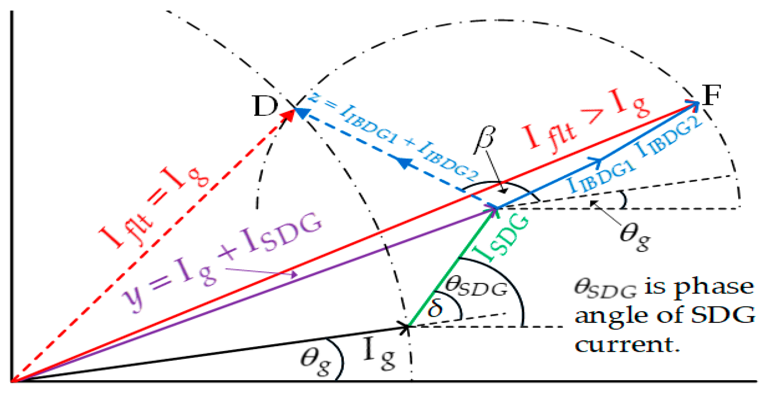
3. Modified Current Phase Angle Calculation

A modified current phase angle calculation can avert an improper current phase angle caused by a fixed Δ because it is performed without the assumption of the fixed Δ. The principle of the modified current phase angle calculation is explained using the phasor diagram in Figure 1. Before the modified current phase angle calculation is applied, the total fault current amplitude at point F is higher than the grid current amplitude. When the current phase angle of IBDGs is tuned to the summation of the phase angle of grid current ( θ g ) and the β angle, the total fault current amplitude is reduced to the grid current amplitude at point D. The modified current phase angle can be expressed as follows:
θ I B D G = θ g + β ,
β = c o s 1 [ I g 2 y 2 z 2 2 y z ] s i n 1 [ I g y s i n ( δ ) ] + δ ,
where y is the summation of the grid current and fault current from the SDG, z is the result of the summation of all currents fed by IBDGs, and δ is the angular difference between the grid current and fault current from the SDG.
Initially, the modified current phase angle calculation is examined based on symmetrical fault. When the fault is detected, the current amplitude is set to the constant that is the maximum allowable current level of the inverter, and the calculation of the current phase angle reference is based on Equation (6). The current phase angle difference between three phases is 120°. This adjustment is called the conventional current control.
Because the V d c is controlled via an active current ( I d ) proportional to the active power, the calculation of the current reference has to take V d c into account. However, for conventional current control, the three-phase current references rely on Equation (6) due to constant current amplitude. Since Equation (6) is not a function of V d c , the conventional current control cannot regulate V d c . In reality, the excessive V d c possibly occurs during a fault. It causes an IBDG disconnection from the grid. The IBDGs fail to remove the effects of fault current contribution from the SDG. Consequently, the coordination then no longer exists in the recloser–fuse.

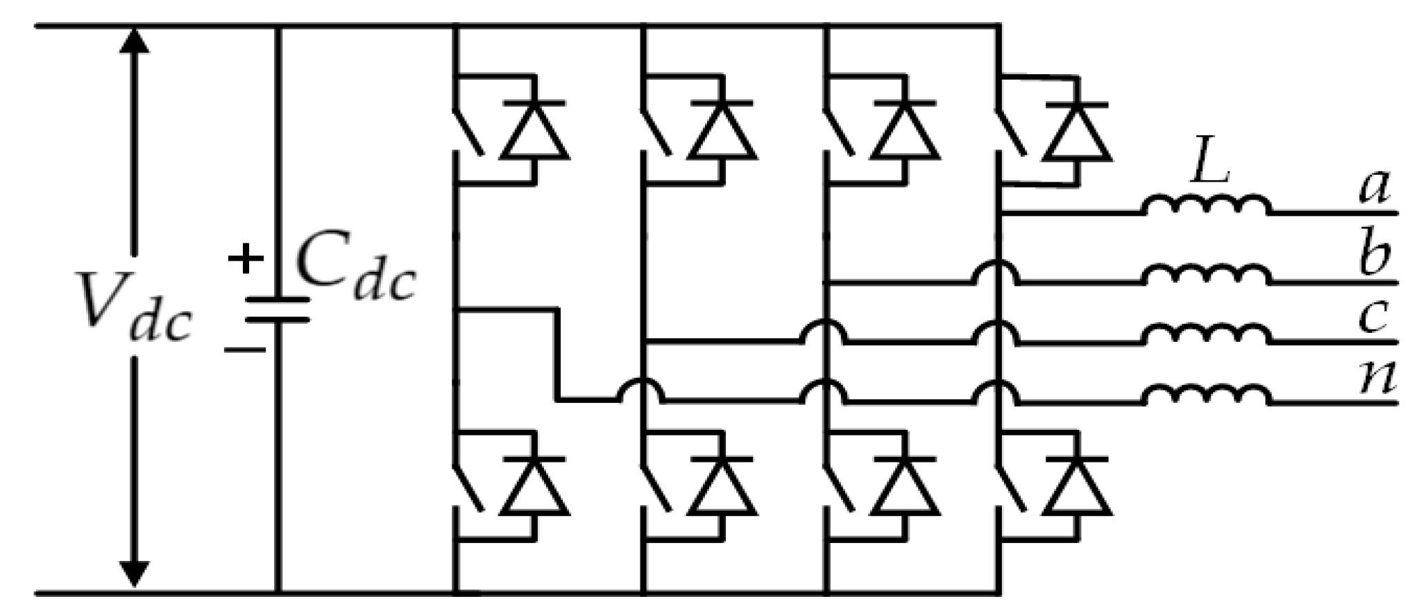
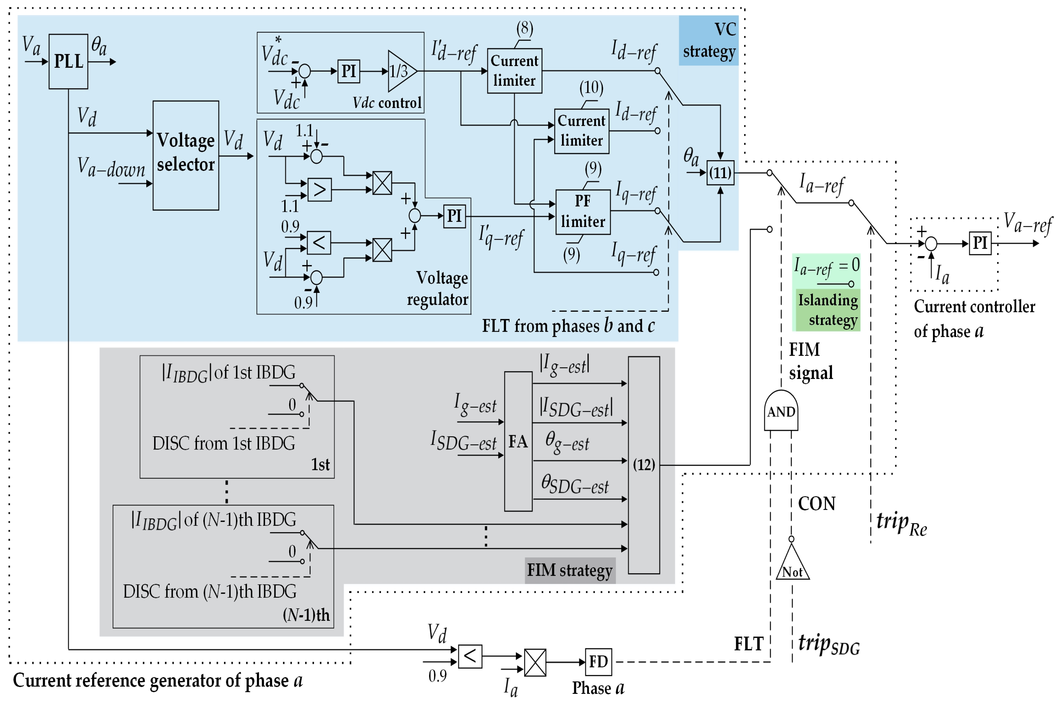
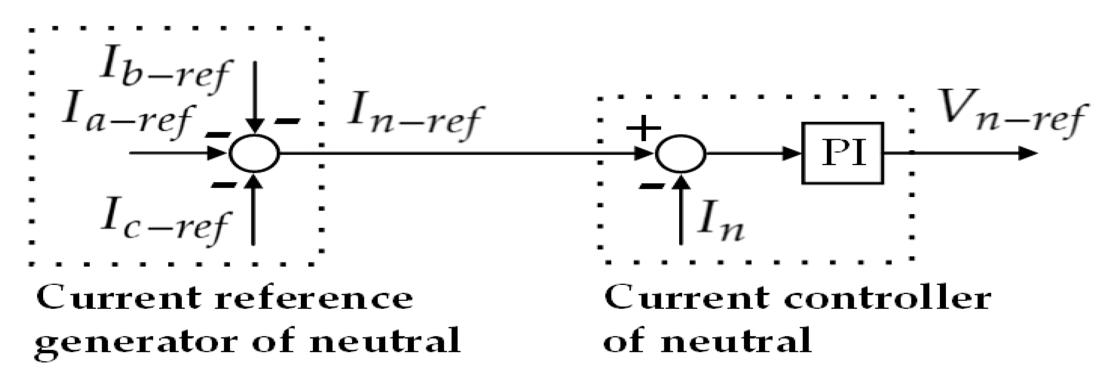
4. Separated Phase–Current Control Using IBDGs

The most common faults in a typical distribution system are unsymmetrical faults [24]. To maintain recloser–fuse coordination and regulate V d c and the grid voltage during the occurrence of these unsymmetrical faults, separated phase–current control using IBDGs is proposed.
Under separated phase–current controls, the current reference of the nonfaulty phase is not reliant on Equation (6) because the protective device in the nonfaulty phase is hardly affected by unsymmetrical faults. The current reference of each nonfaulty phase is mainly determined depending on V d c and the voltage deviation in that phase. This action is to avoid excessive V d c and regulate the grid voltage of each nonfaulty phase. Hence, to realize the separated phase–current control, the three-phase currents are controlled independently. The separated phase–current control is applied with four-leg IBDGs. The topology of the four-leg inverter is shown in Figure 2.
The control diagram of the separated phase–current control for phase a is illustrated in Figure 3. Similarly, the separated phase–current controls for phases b and c are implemented in the same fashion. The separated phase–current control for phase a consists of the current reference generator, current controller, and fault detection (FD) module. The current reference generator includes three strategies, namely voltage control (VC), fault impact mitigation (FIM), and islanding strategies. The VC and FIM strategies are switched depending on the FIM signal resulting from the logical multiplication of the fault signal (FLT) and the SDG connection signal (CON). The FD module detects the fault by considering the transient monitoring function (TMF) [25]. If the d-axis voltage ( V d ), which is computed by the terminal voltage, is below 0.9 per unit (pu), the current feedback is sent to the FD module. It is used for computing the TMF in the FD module. When the calculated TMF exceeds the predefined threshold, the fault is detected. Then, the FD module sends the fault signal to the current reference generator. Otherwise, the connection status of the SDG is recognized by considering the tripping signal sent by the SDG breaker ( t r i p S D G ) . The tripping signal passes through the NOT gate before it reaches the current reference generator. While the SDG is connected to the grid, the NOT gate does not receive any tripping signal. Thus, there is a high signal produced by the NOT gate. This high signal is named the SDG connection signal.
When the AND gate of the current reference generator obtains both the fault signal and SDG connection signal, it generates the FIM signal. Then, the VC strategy is switched to the FIM strategy. On the other hand, the VC and FIM strategies are changed to the islanding strategy when the current reference generator receives the tripping signal sent from the recloser ( t r i p R e ). Teleprotection is applied for sending the tripping signal of the SDG breaker and recloser. Due to the smart grid communication, utilizing the teleprotection is feasible.
For the nonfaulty phase, the FIM signal is not generated due to no fault signal being sent from the FD module. The VC strategy, therefore, is enabled. The VC strategy consists of the V d c control, voltage regulator, current limiters, power factor (PF) limiter, voltage selector, and phase-locked-loop (PLL) control. The active current reference ( I d r e f ) is provided by the V d c control. To regulate V d c , a PI controller is simply adopted to compensate for the error between the DC-link voltage reference ( V d c * ) and the feedback [20]. The voltage regulation feature is performed by the voltage regulator. The voltage regulator gives the reactive current reference ( I q r e f ) for regulating the grid voltage [26]. The dead band of the voltage regulator is in a range of 0.9 to 1.1 pu, which is the acceptable voltage limit according to EN50160 and ESKASAA18 [17]. When V d is out of the dead band, the error between V d and the permissible voltage limit is sent to the PI controller. The output of the PI controller is set as I q r e f . During no fault occurrence, the PF should be varied within a given range defined by the grid code. The inverter must have enough leverage for a reactive current ( I q ), allowing for a minimum PF that complies with the grid code. Thus, the final active current reference ( I d r e f ) is constrained by the current limiter, defined as
I d r e f PF I m a x ,
where I m a x is the maximum allowable current level of the inverter. To satisfy the PF requirement, the final reactive current reference ( I q r e f ) is limited by the PF limiter, defined as
I q r e f t a n ( c o s 1 PF ) I d r e f   ;   PF > 0 I q r e f t a n ( c o s 1 PF ) I d r e f   ;   PF < 0 .
During the ground fault, the grid overvoltage probably occurs in the nonfaulty phase due to the system grounding [27]. It can also be compensated for through deployment of the voltage regulator. For example, grid overvoltage occurs in phase a. If the ground fault occurring in phases b and c causes the grid overvoltage of phase a, the FD module contained in the separated phase–current control of phases b and c sends the fault signal to the current reference generator of phase a. At this moment, the voltage regulation is the top priority. I q r e f is not limited by Equation (9), i.e., I q r e f = I q r e f . Even though an overloaded distribution transformer caused by a lower PF may happen, this does not affect the lifetime of the distribution transformer. This is because the distribution transformer can normally sustain the overloading condition for half an hour [28]. However, the phase current may be greater than the current rating of the power semiconductor. To prevent damage of the inverter, the I d r e f must be restricted by a current limiter, defined as
I d r e f ( I m a x ) 2 ( I q r e f ) 2 .
If the grid overvoltage of phase a is not caused by the ground fault occurring in phases b and c, there is no fault signal from the FD module contained in the separated phase–current control of phases b and c. The overvoltage that is not related to the ground fault may be longer than half an hour. To forbid long-time overload of the distribution transformer caused by a lower PF, both I d r e f and I q r e f are governed by Equations (8) and (9). When both I d r e f and I q r e f are achieved, they are transformed into the phase current reference ( I x r e f ) by
I x r e f = ( I d r e f ) 2 + ( I q r e f ) 2 s i n ( θ x + t a n 1 I q r e f I d r e f ) ,
where subscript x represents phases a, b, and c. The phase voltage ( V x ) is sent to the PLL control to calculate the voltage phase angle ( θ x ). Although the downstream grid voltage exceeds the acceptable voltage limit, the reactive current of the upstream IBDG may be low, because the difference between V d of the upstream IBDG and the acceptable voltage limit used for computing the reactive current reference is not significant. The upstream IBDG contributes to regulating the downstream grid voltage by using the V d of the downstream IBDG as the input of the voltage regulator of the upstream IBDG. The voltage selector switches the input of the voltage regulator between the V d of the upstream IBDG and the V d of the downstream IBDG. A control diagram of the voltage selector is shown in Figure 4.
The sampled phase voltage of the downstream IBDG ( V x d o w n ) is transferred to the upstream IBDG via smart grid communication. When this voltage reaches the upstream IBDG, it is transformed into V d by Park’s transformation. The switching operation of the voltage selector is dependent on a trigger signal. If the V d of the upstream IBDG lies within the permissible voltage limit and the V d of the downstream IBDG is over the admissible voltage limit for longer than 0.05 s, a trigger signal is produced. Then, the V d of the downstream IBDG is chosen as the input of the voltage regulator of the upstream IBDG. The reactive current of the upstream IBDG increases.
For the faulty phase, the current reference generator is divided into two circumstances. The first circumstance is already explained. The AND gate generates the FIM signal as it receives both the fault signal and SDG connection signal. The FIM strategy is enabled to eliminate the effects of fault current contribution from the SDG. The phase current reference is calculated by
I x r e f = I m a x s i n [ 2 π f t + θ g e s t + β ] ,
where f is the grid frequency and θ g e s t is the phase angle of the estimated grid current. The details of the grid and SDG current estimations will be explained in Section 6. When the estimated grid current ( I g e s t ) and estimated SDG current ( I S D G e s t ) are achieved, they are sent to the Fourier analysis (FA) module contained in the FIM strategy. The FA module extracts the amplitude of the estimated grid and SDG currents ( | I g e s t | and | I S D G e s t | ) and the phase of the estimated grid and SDG currents ( θ S D G e s t ) (Equation (12)). The β angle can be calculated by using Equation (7). The current amplitude of the IBDGs ( | I I B D G | ) connected to grid is used in the calculation. Thus, to correctly calculate the β angle in the case of some IBDGs being disconnected from the grid, the IBDGs should recognize the disconnection. The disconnection signal (DISC) of the IBDGs can be obtained through smart grid communication. If some IBDGs are disconnected, the disconnection signals are sent. Their current amplitudes for calculating the β angle are set at zero. N stands for the number of IBDGs installed in the system. As a consequence, the β angle calculation is still correct, although there is a disconnection for some IBDGs. On the other hand, for the second circumstance, the AND gate receives only the fault signal sent from the FD module, since the SDG is disconnected from the grid. Hence, there is no FIM signal produced by the AND gate, and the VC strategy is enabled.
For the isolated phase, the islanding strategy is activated because of the tripping signal sent by the recloser. The phase current reference is set at zero in order to prevent the damages caused by out-of-phase reclosing.
A control diagram of the current control for “neutral” connected to the fourth leg of the IBDG is shown in Figure 5. When three-phase current references are prepared, they are combined with a negative sign. This summation is set as the current reference for “neutral” ( I n r e f ). Finally, in Figure 3 and Figure 5, the three-phase current references and neutral current reference are sent to the PI current controller. In the phase current regulation, the PI controller compensates for the error between the phase current reference and phase current feedback ( I x ). Similarly, a PI controller is also adopted for the neutral current ( I n ) regulation. The outputs of the PI controllers for the phase and neutral currents consist of the phase voltage reference ( V x r e f ) and neutral voltage reference ( V n r e f ), respectively. The voltage references are applied in generating the pulse width modulation (PWM) signal.
As a consequence of the presence of an individual current reference generator and current controller in each phase, three-phase currents can be controlled independently. The operation of IBDGs is flexible due to three strategies of the current reference generator. If the energy is continuously accumulated in the DC-link capacitor ( C d c ), an excessive V d c may occur. This results in the disconnection of IBDGs. A VC strategy can avoid the disconnection of IBDGs caused by excessive V d c , since the energy of C d c is transferred to the grid by injecting the active current. Additionally, the VC strategy controls the reactive current to regulate the grid voltage. Otherwise, the recloser–fuse miscoordination and the damages caused by out-of-phase reclosing can be prevented by FIM and islanding strategies.

5. Delay Caused by Using PMUs

PMUs have been found in many applications in distribution systems. The use of PMUs can introduce a delay in real-time applications [29]. The sources of PMU measurement delay include PMU processing, phasor data concentrator (PDC) processing, communications protocols, and networks being used to transfer measurement data. The delayed measurements can greatly affect the accuracy of real-time state estimation and control schemes, particularly in the presence of faults. For example, in wide-area voltage control [30], the voltage data sent by PMUs are used to compute the current reference. With the delayed PMU data, the controller receives the delayed voltage signal and processes the real-time voltage. This results in an error in the current reference, and consequently the obtained voltage profile oscillates. The performance of the wide-area voltage control is degraded. The PMU processing, PDC processing, and propagation delays are constant. On the other hand, the serial and routing delays are considered to be stochastic delay. The mean ( M ¯ ) and standard deviation (σ) values of the serial delay are set at 20 µs and 8.944 µs, respectively [31]. The M ¯ and σ of the routing delay are found by means of a Monte Carlo simulation with a routing delay equation. The routing delay ( τ r o u t ) is expressed as
τ r o u t = λ λ ( ζ λ ) ,
where λ is the incoming data rate (bits/s) and ζ is the serving data rate (bits/s). The M ¯ and σ of the coming data rate are 12,000 bits/s and 5366.56 bits/s, respectively [31]. The serving data rate is defined as 10 Mbits/s. After the Monte Carlo simulation randomly samples the incoming data rate 100,000 times, this results in an M ¯ and σ of the routing delay of 0.1 µs and 0.05404 ns, respectively. M ¯ and the variance (σ2) are used as the inputs of a Gaussian probability distribution function, which generates random values of serial and routing delays [32]. These delays are assigned to every sending packet.

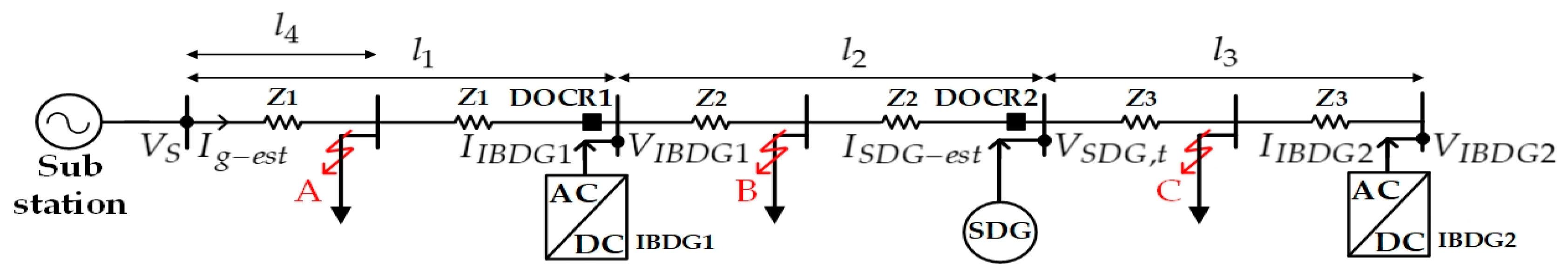
6. Grid and SDG Current Estimations

The time delay of using PMUs can significantly affect the FIM strategy of separated phase–current control because it needs data from the grid and SDG currents for calculating the current reference. To avoid this delay, this paper also presents the grid and SDG current estimations programmed into the IBDGs.
The grid and SDG current estimations can be divided into three cases depending on the fault section, as shown in Figure 6. Z1, Z2, and Z3 are impedance per length. Each fault section is distinguished by considering the signal of the directional overcurrent relay (DOCR) placed at the IBDG1 and SDG nodes. Sending the relay signal is carried out by teleprotection. If a fault occurs at point C in the section next to the SDG, IBDG1 and IBDG2 receive the relay signals from both DOCR1 and DOCR2. If the fault is at point B in the section between IBDG1 and SDG, the relay signal is sent by only DOCR1. When the fault occurs upstream of the DOCR, for instance at point A, no relay signal is transmitted by either DOCR1 or DOCR2. Besides, current estimations require the sampled voltage and current data of the IBDGs. These sampled values can be exchanged between IBDGs through smart grid communication.

6.1. Fault in the Section behind the SDG (Point C)

The grid current is estimated from the relationship between the substation voltage ( V S ) and the voltage of IBDG1 ( V I B D G 1 ). The estimated grid current is expressed as
I g e s t = [ Z 1 l 1 ] 1 [ V S V I B D G 1 ] ,
where l 1 is the line length between the substation and IBDG1. On the other hand, the SDG current in the stator, field, and damper windings can be computed from a state–space (SS) equation of a synchronous machine (SM). The SS equation using the dq-axis current ( I S D G , d q ) as a state variable is expressed as the following equations:
I ˙ S D G , d q = L S D G 1 [ R S D G + ω L S D G ] I S D G , d q L S D G 1 V S D G , d q ,
I S D G , d q = [ I s q I s d I f d I k d I k q ] ,
V S D G , d q = [ V t q V t d V f d V k d V k q ] ,
R S D G = [ R s 0 0 0 0 0 R s 0 0 0 0 0 R f d 0 0 0 0 0 R k d 0 0 0 0 0 R k q ] ,
L S D G = [ L q 0 0 0 L m q 0 L d L m d L m d 0 0 L m d L f d L m d 0 0 L m d L m d L k d 0 L m q 0 0 0 L k q ] ,
ω = [ 0 ω r 0 0 0 ω r 0 0 0 0 0 0 0 0 0 0 0 0 0 0 0 0 0 0 0 ] .
The dynamics of the stator, field, and damper windings are taken into account. The SS equation can represent the dynamic behavior of the SM. The state variables of the SS include a dq-axis stator current ( I s d and I s q ), a d-axis field current ( I f d ), and a dq-axis damper winding current ( I k d and I k q ). The dq-axis voltage ( V S D G , d q ) matrix consists of a dq-axis terminal voltage ( V t d and V t q ), d-axis field voltage ( V f d ) , and dq-axis damper winding voltage ( V k d and V k q ). The resistance ( R S D G ) is the diagonal matrix, including stator resistance ( R s ), d-axis field resistance ( R f d ), and dq-axis damper winding resistance ( R k d and R k q ). The inductance ( L S D G ) matrix consists of dq-axis inductance ( L d and L q ) , d-axis field inductance ( L f d ), dq-axis damper winding inductance ( L k d and L k q ), dq-axis mutual inductance ( L m d and L m q ), and zero elements. The angular velocity ( ω ) matrix is built from angular rotor speed ( ω r ) and zero elements. According to Equation (15), dq-axis terminal voltage, dq-axis damper winding voltage, d-axis field voltage, angular rotor speed, resistance, and inductance are needed. The three-phase terminal voltage of SDG ( V S D G , t ) can be calculated from
V S D G , t = V I B D G 1 [ Z 2 l 2 ] [ I g e s t + I I B D G 1 ] ,
where l 2 defines the line length between IBDG1 and the SDG. I I B D G 1 is the current of IBDG1. When the three-phase terminal voltage is obtained, it is transformed from its a–b–c frame to its d–q frame. The dq-axis damper winding voltage is defined as zero due to the closed conducting path on the rotor. Otherwise, the d-axis field voltage and angular rotor speed are set at a nominal value. The resistance and inductance are known parameters. When the dq-axis stator current is achieved from the SS equation, it is transformed back from a d–q frame into an a–b–c frame. This transformed current is used as the estimated SDG current. Finally, both the estimated grid and SDG currents are sent to the FIM strategy, as shown in Figure 3.

6.2. Fault in the Section between IBDG1 and the SDG (Point B)

Similarly to the previous case, the grid current is estimated by using Equation (14), and the SS equation is used for estimating the SDG current. However, the three-phase terminal voltage of the SDG is calculated by Equation (22) instead:
V S D G , t = V I B D G 2 [ Z 3 l 3 ] [ I I B D G 2 ] ,
where l 3 is the line length between the SDG and IBDG2. V I B D G 2 and I I B D G 2 are the voltage and current of IBDG2, respectively.

6.3. Fault in the Section in Front of IBDG1 (Point A)

Similarly, the SDG current is estimated by the SS equation, and the three-phase terminal voltage of the SDG is calculated by Equation (22). Otherwise, the grid current is estimated based on fault point voltage. The fault point voltage on the substation ( V S F ) and the fault point voltage on IBDG1 ( V I B D G 1 F ) are expressed as follows:
V S F = V S [ Z 1 l 4 ] [ I g e s t ] ,
V I B D G 1 F = V I B D G 1 [ Z 1 ( l 1 l 4 ) ] [ I I B D G 1 + I I B D G 2 + I S D G e s t ] ,
where l 4 is the line length between the substation and fault point. Because the fault point voltage on the substation and the fault point voltage on IBDG1 are equal, the grid current can be estimated by
I g e s t = [ Z 1 l 4 ] 1 [ V S V I B D G 1 ] + [ Z 1 l 4 ] 1 [ Z 1 ( l 1 l 4 ) ] [ I I B D G 1 + I I B D G 2 + I S D G e s t ] .
Nevertheless, the fault point found is beyond the scope of this paper. The approach for finding the fault point will be studied in future work.
For the different distribution systems, the estimated grid current equation may be revised; however, it is still derived by using Kirchhoff’s voltage law. Conversely, the same SS equation can be used to estimate the SDG current.

7. Simulation Assessment

Simulations are commonly used in power system research because they can minimize cost and time. MATLAB/Simulink (2019b, The MathWorks, Inc., Natick, MA, USA, 2019) [33] was adopted in this work. It was designed for both modeling the electrical power system and developing the control algorithm. The proposed algorithm can be implemented in readily existing models in the software. A simulation study was performed on an IEEE 34-node radial test feeder to assess the dynamic performances of the proposed separated phase–current control using IBDGs, as shown in Figure 7a. The system parameters are listed in Reference [34]. IBDG1 and IBDG2 were connected at nodes 816 and 860, respectively. During voltage sag, the DC–DC boost converter connecting the photovoltaics (PV) and IBDGs is operated under a power balance strategy to avoid an imbalance between the input power and output power of the IBDGs [20]. The total penetration level of the two IBDGs was 54% of power demand. The output current of the IBDGs was limited to within 2 times of the rated current of the switching device to prevent damage to the inverter [15,18]. A 0.8-MVA SDG was connected at node 828. A fiberoptic communication was assumed as the means for the main data transmission due to the benefits of high bandwidth capacity and electromagnetic interference (EMI)/radio frequency interference (RFI) immunity. More importantly, optical fibers have already been widely adopted in communication networks [35]. The propagation speed and data rate were 4.978 μs/km and 10 Mbits/s, respectively. Three single-phase reclosers (Res) installed in the substation and a fuse (F) placed at the beginning of lateral 7 were used to investigate the effects of fault current contribution from the SDG. The benefit of three single-phase reclosers is that the utility still supplies the nonfaulty phase during unsymmetrical faults [3]. The number of customers affected by outages can be reduced. The corresponding time–current curve of the recloser–fuse is shown in Figure 7b. A fuse-saving philosophy is commonly used by allowing circuit breaker relays and recloser controls to trip before the fusible element starts melting, which is indicated by the fast curve below the fuse characteristic in Figure 7b. After the first or second reclosing attempts, the relays turn to the slow curve, coordinated to allow the fuse to melt before the recloser trips to restore service to the rest of the feeder. The simulation assessment is divided into two parts. The impact of delay caused by the PMUs is validated in the first part. The second part evaluates the efficiency of separated phase–current controls.

7.1. Effects of Delay Caused by PMUs

PMUs were installed at the substation and SDG to monitor the grid and SDG currents. The PDC for collecting the data sent by PMUs was placed at the substation. The total delay of using PMUs was a combination of PMU processing, PDC processing, and serial, routing, and propagation delays. The PMU processing and PDC processing delays were set at 26 ms and 80 ms, respectively [36]. The serial and routing delays were determined in Section 5. The propagation delay was obtained by the propagation speed and total distance. The total distance was the sum of the distance from the PMUs to the PDC and the distance from the PDC to the IBDGs. The shorter the total distance was, the lower the propagation delay was. The propagation delays from the PMUs located at the substation to IBDG1 (32 km) and IBDG2 (57 km) were 0.16 ms and 0.285 ms, respectively. On the other hand, the propagation delays from the PMUs installed at the SDG to IBDG1 (67 km) and IBDG2 (92 km) were 0.335 ms and 0.46 ms, respectively.
The single line to ground (SLG) fault was estimated at 80% for all kinds of fault occurrences [24]. From 0.14 to 0.44 s, phase b was short-circuited to the ground with 0.01 Ω of fault resistance ( R f ) in the section between nodes 834 and 842. The fault was detected by IBDGs, and the FIM strategy of separated phase–current controls was enabled at 0.155 s. The grid and SDG currents computed by PMU data are shown in Figure 8a. After the fault was detected, the grid and SDG currents computed by PMU data were noticeably different from the real-time grid and SDG currents as a result of the delay. This resulted in an error in the current reference of the FIM strategy calculated by using the PMU data. The total fault current amplitude was not reduced to the grid current amplitude, as shown in Figure 8b. Several cycles later, the grid and SDG currents computed by the PMU data became close to the real-time grid and SDG currents. The total fault current amplitude was decreased to the grid current amplitude. Nevertheless, it was too late because the fuse melted before the recloser operated, as shown in Figure 8c. The recloser–fuse coordination was thus compromised.

7.2. Performance of the Separated Phase–Current Controls Using IBDGs

This section compares the effectiveness of the separated phase–current controls and conventional current controls to the temporary SLG fault and temporary line-to-line (LL) fault. The temporary fault duration was assumed to be 0.3 s. Moreover, the separated phase–current controls were examined under permanent SLG faults. Both temporary and permanent faults occurred in the section between nodes 834 and 842. The use of PMUs was replaced by integrating the grid and SDG current estimations into the IBDGs. Like the merging unit (MU), the sampled value exchanged between the IBDGs for estimations was directly mapped into the ethernet frame. Due to the unavailability of stochastic serial delay in all studies, the total delay was computed by combining the processing and end-to-end (ETE) delays. The processing delay was determined to be 1.05 ms [37]. The ETE delay was considered to be random, with the mean value, M ¯ , and standard deviation, σ, at 0.2019 ms and 0.0119 ms, respectively [38]. The M ¯ and variance, σ2, were applied as the input of the Gaussian probability distribution function to generate random values of the ETE delay. The ETE delay was presumably based on short-distance communication, and the propagation delay was negligible. Thus, the propagation delay between the two IBDGs (25 km) was included in the total delay. That propagation delay was 0.125 ms.

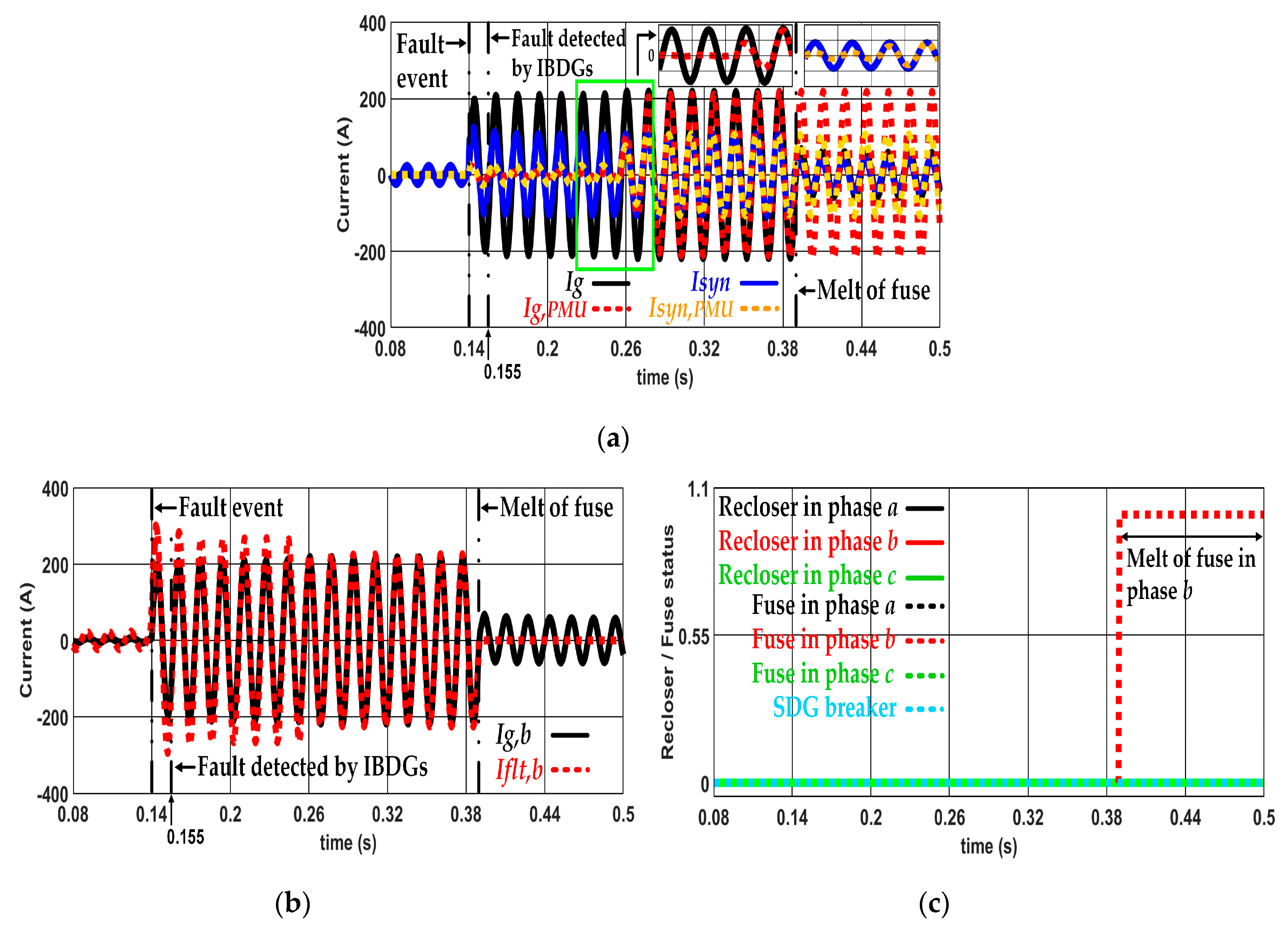
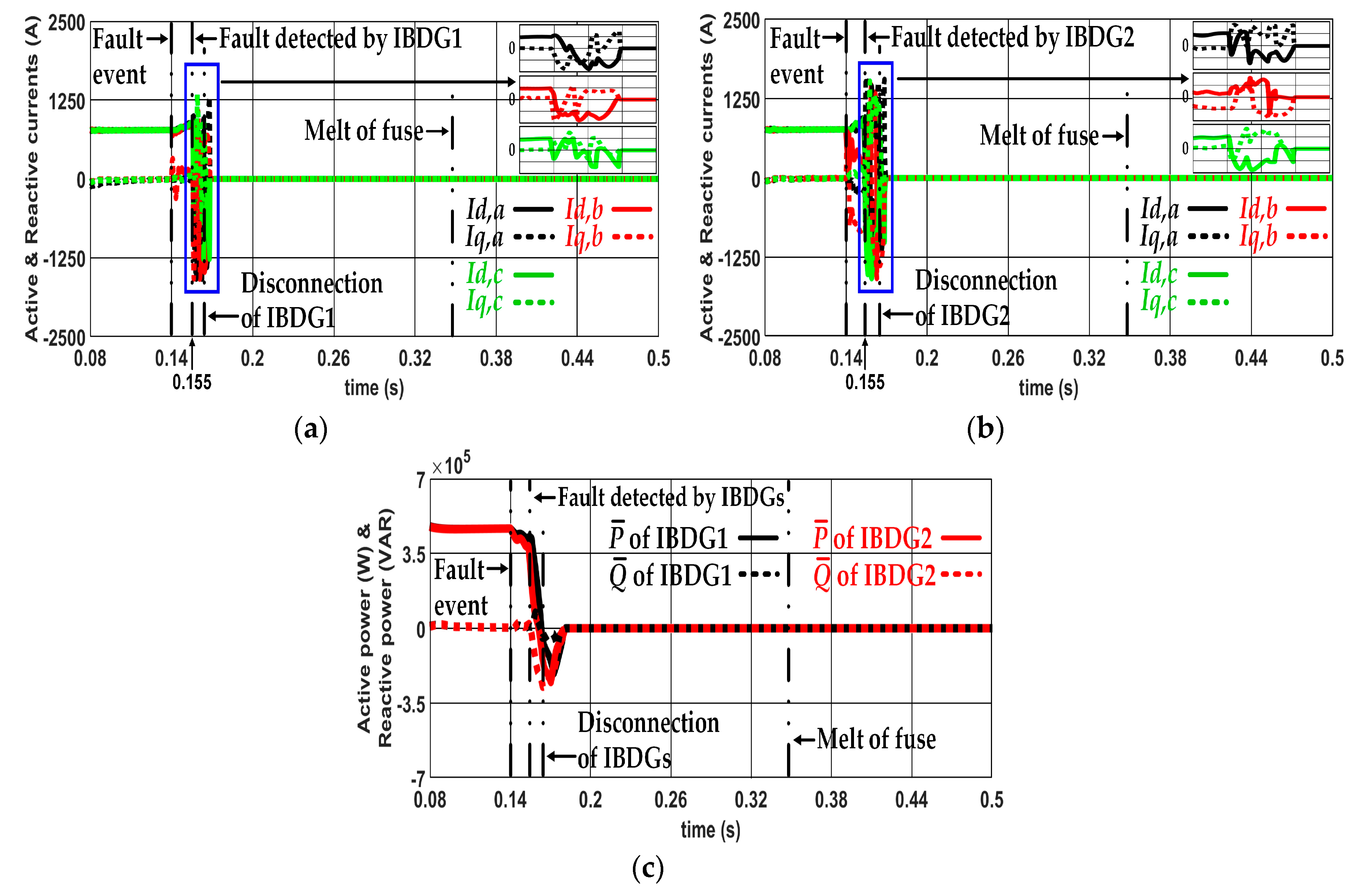
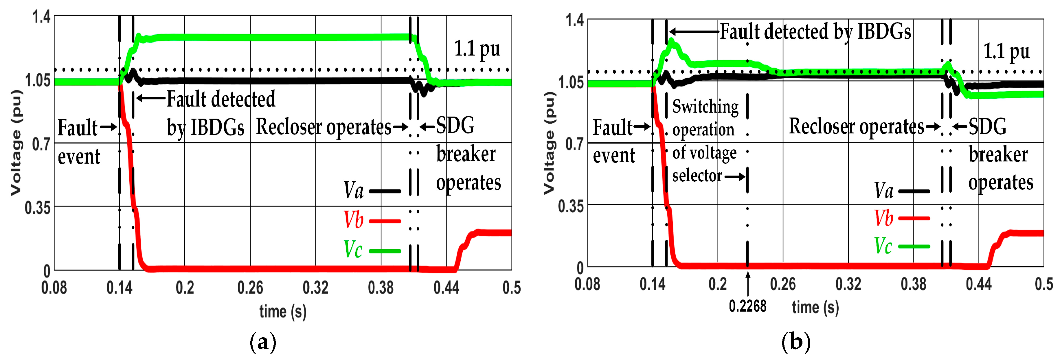
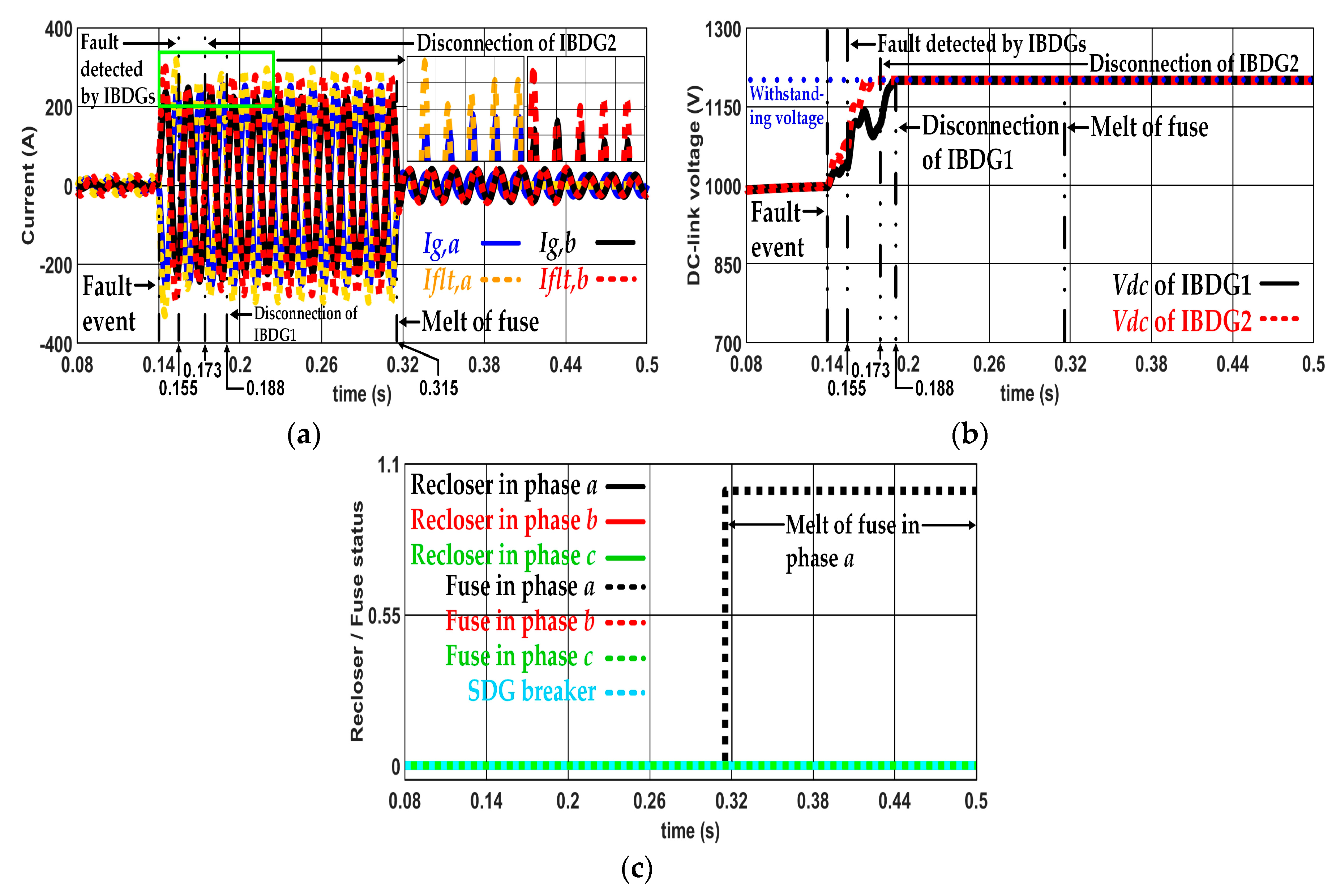
7.2.1. Temporary SLG Fault

The SLG fault was created by short-circuiting phase b to the ground with 0.01 Ω of R f . As shown in Figure 9a, the total fault current amplitude was higher than the grid current amplitude after the fault occurred at 0.14 s. When the fault was detected at 0.155 s, the total fault current amplitude was equated to the grid current amplitude by conventional current controls. Soon after, in Figure 9b, V d c reached the withstanding voltage of C d c at 1.2 times the operating voltage (i.e., 1200 V) [39]. Consequently, the IBDGs were disconnected from the grid at 0.164 s, and the total fault current amplitude became greater than the grid current amplitude once again. As shown in Figure 9c, the fuse melted at 0.348 s before the tripping operation of the recloser and the recloser–fuse were no longer coordinated. After the fuse melted at 0.348 s, the grid current was substantially reduced.
In Figure 10a, the separated phase–current control effectively reduced the total fault current amplitude to the grid current amplitude immediately after the fault was detected at 0.155 s. The estimated grid and SDG currents used for calculating the current reference are shown in Figure 10b. The estimated currents were equivalent to the real-time currents after the fault was detected. The current reference, thus, could be calculated correctly. The V d c regulation within the withstanding voltage at 1200 V is illustrated in Figure 10c. The disconnection of IBDGs caused by excessive V d c was avoided. As shown in Figure 10d, the tripping operation of the recloser occurred prior to the melting of the fuse, i.e., the recloser–fuse coordination was preserved. If the recloser trips, the IBDGs and SDG should be disconnected to prevent damage caused by out-of-phase reclosing. By applying the teleprotection, the IBDGs and SDG breaker received the tripping signal sent by the recloser. After the tripping event of the recloser and SDG breaker (at 0.406 s and 0.414 s), the total fault current was reduced significantly.
In conventional current control, the active current utilized to transfer the energy in C d c and the reactive current used to regulate the grid voltage are arbitrary. The three-phase current references are reliant on Equation (6), which is obtained by considering only the fault current. As shown in Figure 11a,b, after the fault was detected at 0.155 s, negative IBDG1 currents indicated that the active currents were drawn from phases a, b, and c. At the same time, in IBDG2, the active currents were drawn only from phases a and c. Although the IBDG2 injected a noticeable amount of the active current into phase b, there was hardly any active power transmitted by IBDG2 to the grid due to the deep voltage sag of phase b. In Figure 11c, both IBDGs absorbed the average active power ( P ¯ ) and reactive power ( Q ¯ ) from the grid, an agreement with the active and reactive currents. Consequently, the power was delivered to C d c by IBDGs. The energy was accumulated in C d c and eventually caused excessive V d c during fault.
For the separated phase–current controls, V d c could be lower than the withstanding voltage due to the VC strategy applied in IBDGs. In the nonfaulty phase, the VC strategy was activated. The active and reactive currents were controlled to transfer energy from C d c to the grid and regulate the grid voltage. The energy in C d c was sent to the grid by injecting the active current. As shown in Figure 12a,b, the IBDGs injected the active current into phases a and c. In the faulty phase, the fault and the connection of SDG were detected. The FIM strategy was enabled at 0.155 s to remove the effects of fault current contribution from the SDG. The active and reactive currents behaved rather arbitrarily because the current reference was computed by Equation (12), which is derived from the fault current, where the V d c and grid voltage are not considered. As shown in Figure 12a,b, IBDG1 absorbed the active current from phase b, while IBDG2 injected the active current into phase b. After the tripping event of the recloser at 0.406 s, the FIM strategy was changed to an islanding strategy because the recloser sent a tripping signal to the IBDGs. In other words, no IBDG supplied the active and reactive currents to phase b. This action prevented the damage caused by out-of-phase reclosing. The P ¯ and Q ¯ of all IBDGs can be seen in Figure 12c. Due to the active current injection, all IBDGs could inject the active power into the grid during a fault.
The benefit of the voltage regulation feature is demonstrated in Figure 13 for the three-phase voltages at node 862, where the voltage regulation feature was disabled and enabled. During a ground fault, the grid overvoltage of the nonfaulty phase could occur due to the system grounding. In Figure 13a, the grid voltage in phase c was increased over the upper permissible voltage limit of 1.1 pu since the voltage regulation feature was disabled. When the voltage regulation feature was turned back on, all of the IBDGs compensated for the grid overvoltage of phase c by absorbing the reactive current, as shown in Figure 12a,b. The reactive current of phase c drawn by IBDG2 increased. Because the difference between V d of IBDG1 and the upper permissible voltage limit was small, the IBDG1 consumed a low reactive current from phase c. Although the grid overvoltage of phase c was reduced, it was still higher than the upper permissible voltage limit, as shown in Figure 13b. At 0.2268 s, the voltage selector of IBDG1 switched the input of the voltage regulator from V d of IBDG1 to V d of IBDG2. The reactive current of phase c consumed by IBDG1 increased. Accordingly, the grid overvoltage of phase c could be compensated for at around the upper acceptable voltage limit. From the reactive power relationship ( Q = 0.5 V d I q ), the reactive power flowed from the grid to the IBDGs when the reactive current was controlled as positive, meaning that the reactive current consumed by the IBDGs was of a positive quantity.

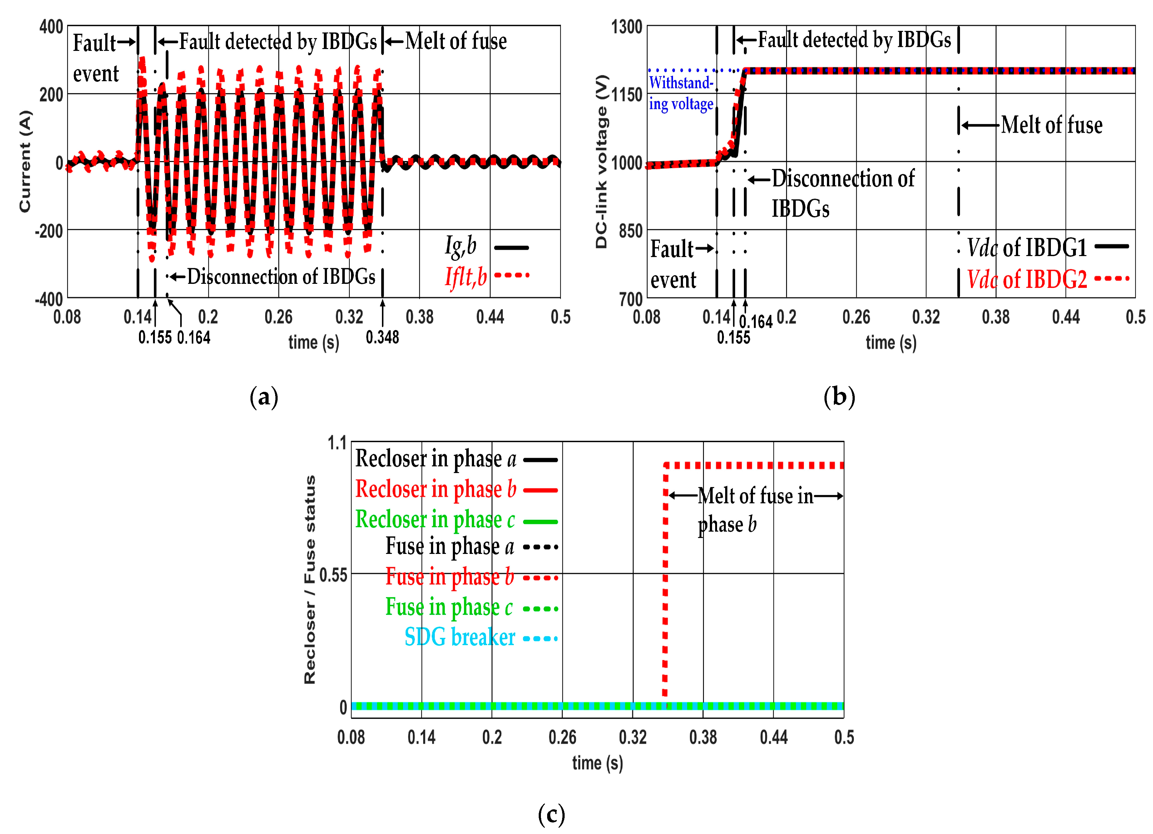
7.2.2. Temporary LL Fault

The LL fault was estimated at 10% for all kinds of fault occurrences [24]. Phases a and b were short-circuited with 0.01 Ω of R f . Figure 14a shows the total fault current compared to the grid current. After the fault occurred at 0.14 s, the total fault current amplitude was greater than the grid current amplitude. When the fault was detected at 0.155 s, the conventional current control decreased the total fault current amplitude to the grid current amplitude. Then, V d c reached the withstanding voltage of C d c , as shown in Figure 14b. IBDG1 and IBDG2 were disconnected from the grid at 0.188 s and 0.173 s, respectively. The cause of excessive V d c was the same as in the previous SLG fault. After the IBDGs were disconnected, the total fault current amplitude became greater than the grid current amplitude again. The operation of the recloser–fuse and SDG breaker is shown in Figure 14c. The recloser–fuse coordination was lost, as the fuse melted before the recloser operated. After the fuse melted at 0.315 s, the grid current and total fault current were greatly decreased.
With the separated phase–current controls, after the fault was detected at 0.148 s, the total fault current amplitude was reduced approximately to the grid current amplitude, as shown in Figure 15a. Since there was no disconnection of IBDGs caused by excessive V d c , the total fault current amplitude remained close to the grid current amplitude until the recloser tripped. V d c was regulated within the withstanding voltage, as shown in Figure 15b. The operations of the recloser–fuse and SDG breaker are shown in Figure 15c. The tripping operation of the recloser happened before the fuse melted; hence, the recloser–fuse coordination remained effective. When the recloser tripped, the SDG breaker operated. After the tripping event of the recloser in phase a and in the SDG breaker at 0.333 s and 0.34 s, respectively, the grid current in phase b was reduced. Similarly, the total fault current in phases a and b also decreased.

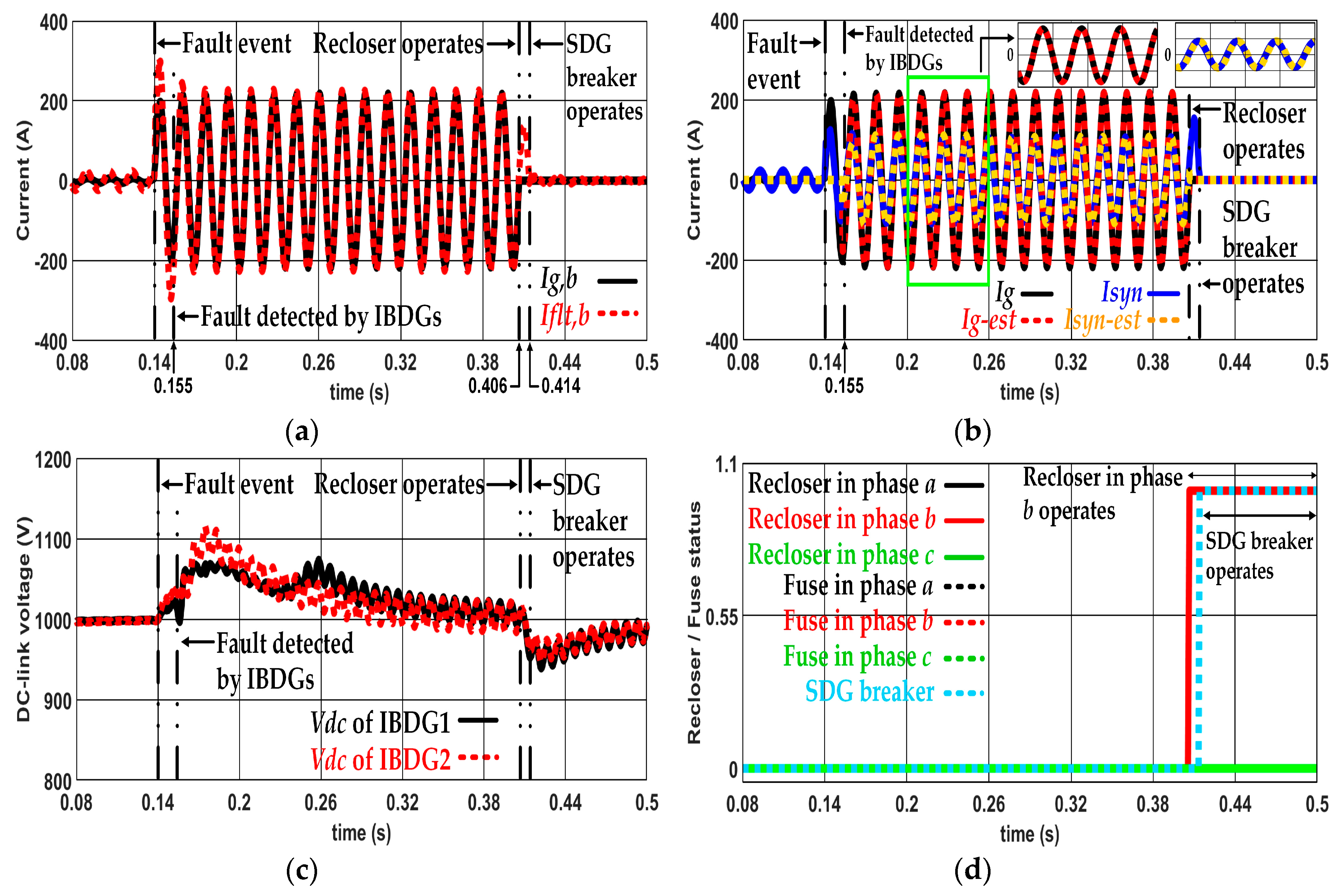
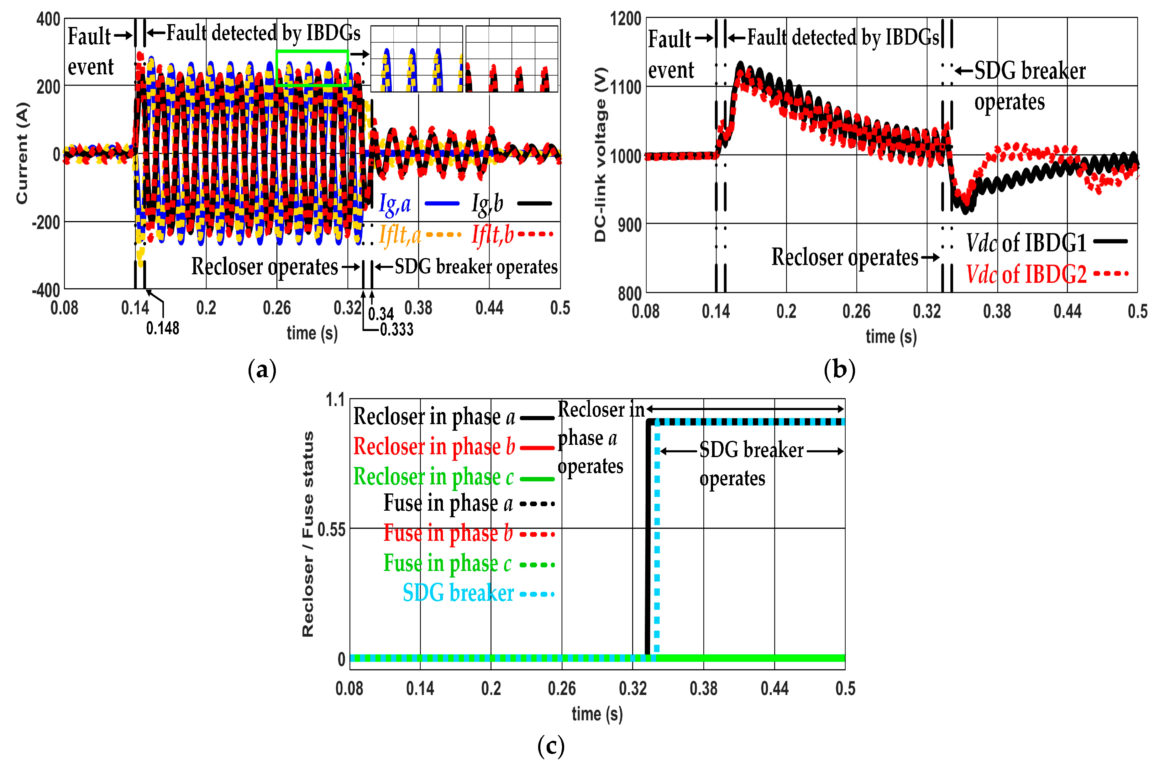
7.2.3. Permanent SLG Fault

The SLG fault was created by short-circuiting phase b to ground with R f of 0.01 Ω. The operation of the recloser–fuse and SDG breaker is shown in Figure 16. The fuse melted prior to the third tripping operation of the recloser. Thus, the separated phase–current control could prevent the miscoordination of the recloser–fuse even during a permanent fault.
These simulation results demonstrated the effectiveness of separated phase–current controls using IBDGs and current estimations. The separated phase–current controls could regulate V d c within the withstanding voltage of C d c . During unsymmetrical faults, there were some ripples that occurred in V d c because of an oscillating power component. This may have led to a distorted current waveform. However, these ripples could be mitigated by introducing the notch filter into the V d c control loop [40]. Due to no disconnection of IBDGs caused by excessive V d c , the IBDGs could reduce the total fault current amplitude to the grid current amplitude without any problem. The recloser–fuse coordination was preserved during temporary and permanent unsymmetrical faults. When the recloser was operated, the current was not supplied from the IBDGs to the isolated phase to avoid the damage caused by out-of-phase reclosing. Not only could this prevent recloser–fuse miscoordination and damage from out-of-phase reclosing, but it could also regulate the grid voltage for a nonfaulty phase. During the SLG fault, the grid overvoltage of the nonfaulty phase was compensated for within the upper permissible voltage limit (1.1 pu) by the voltage regulation feature of the separated phase–current control. Furthermore, the grid and SDG current estimations integrated into the IBDGs could avoid the delay of using PMUs. The estimated grid and SDG currents were equivalent to real-time grid and SDG currents; therefore, there was no error in the current reference calculated by using the estimated currents. The performance of the separated phase–current controls was not degraded.

8. Conclusions

This paper proposed separated phase–current controls using IBDGs. The current reference generator and current controller in each phase are operated independently. The three strategies for the current reference generator result in flexible operation of the IBDGs. The VC strategy controls the active and reactive currents to transfer the energy from C d c to the grid and regulate the grid voltage. The FIM strategy reduces the total fault current contributed by the SDG, and the islanding strategy prohibits the damage due to out-of-phase reclosing. Furthermore, the grid and SDG current estimations are adopted in the IBDGs to avoid the delay in PMU data. The separated phase–current controls using IBDGs, under unsymmetrical faults, were validated through simulations. The results showed that the delay in using PMUs could degrade the effectiveness of the separated phase–current controls. That degradation was removed by means of the current estimations programmed into the IBDGs. Moreover, the separated phase–current controls could maintain V d c below the withstanding voltage of C d c . The disconnection of the IBDGs caused by excessive V d c was addressed. Subsequently, the coordination of the recloser–fuse in the faulty phase was maintained, and the grid voltage in the nonfaulty phase was regulated.

Author Contributions

N.B. (Nattapon Boonyapakdee) proposed the main idea, performed the simulation, and wrote the manuscript. M.K. and A.S. (Mongkol Konghirun and Anawach Sangswang) provided key suggestions and improved the manuscript.

Funding

This research received no external funding.

Conflicts of Interest

The authors declare no conflict of interest.

References

  1. Strezoski, L.V.; Prica, M.D. Short-Circuit Analysis in Large-Scale Distribution Systems with High Penetration of Distributed Generators. IEEE/CAA J. Autom. Sin. 2017, 4, 243–251. [Google Scholar] [CrossRef]
  2. Girgis, A.; Brahma, S. Effect of Distributed Generation on Protective Device Coordination in Distribution System. In Proceedings of the 2001 Large Engineering Systems Conference on Power Engineering, Halifax, NS, Canada, 11–13 July 2001. [Google Scholar]
  3. Gers, J.M.; Holmes, E.J. Protection of Electricity Distribution Networks, 3rd ed.; IET: London, UK, 2011. [Google Scholar]
  4. Chaitusaney, S.; Yokoyama, A. Prevention of Reliability Degradation from Recloser-Fuse Miscoordination Due To Distributed Generation. IEEE Trans. Power Deliv. 2008, 23, 2545–2554. [Google Scholar] [CrossRef]
  5. Abdel-Ghany, H.A.; Azmy, A.M.; Elkalashy, N.I.; Rashad, E.M. Optimizing DG Penetration in Distribution Networks Concerning Protection Schemes and Technical Impact. Elect. Power Syst. Res. 2015, 128, 113–122. [Google Scholar] [CrossRef]
  6. Shah, P.H.; Bhalja, B.R. New Adaptive Digital Relaying Scheme to Tackle Recloser-Fuse Miscoordination during Distributed Generation Interconnections. IET Gener. Transm. Distrib. 2014, 8, 682–688. [Google Scholar] [CrossRef]
  7. Jamali, S.; Borhani-Bahabadi, H. Recloser Time-Current-Voltage Characteristic for Fuse Saving in Distribution Networks with DG. IET Gener. Transm. Distrib. 2017, 11, 272–279. [Google Scholar] [CrossRef]
  8. Liu, Z.; Su, C.; Høidalen, H.K.; Chen, Z. A Multiagent System-Based Protection and Control Scheme for Distribution System with Distributed-Generation Integration. IEEE Trans. Power Deliv. 2017, 32, 536–545. [Google Scholar] [CrossRef]
  9. Park, W.J.; Sung, B.C.; Park, J.W. The Effect of SFCL on Electric Power Grid with Wind-Turbine Generation System. IEEE Trans. Appl. Supercond. 2010, 20, 1177–1181. [Google Scholar] [CrossRef]
  10. Fereidouni, A.R.; Vahidi, B.; Mehr, T.H. The Impact of Solid State Fault Current Limiter on Power Network with Wind-Turbine Power Generation. IEEE Trans. Smart Grid 2013, 4, 1188–1196. [Google Scholar] [CrossRef]
  11. Yazdanpanahi, H.; Xu, W.; Li, Y.W. A Novel Fault Current Control Scheme to Reduce Synchronous DG’s Impact on Protection Coordination. IEEE Trans. Power Deliv. 2014, 29, 542–551. [Google Scholar] [CrossRef]
  12. Ustun, T.S.; Ozansoy, C.; Zayegh, A. A Central Microgrid Protection System for Networks with Fault Current Limiters. In Proceedings of the 2011 10th International Conference on Environment and Electrical Engineering, Rome, Italy, 8–11 May 2011. [Google Scholar]
  13. Liang, Z.; Lin, X.; Kang, Y.; Gao, B.; Lei, H. Short Circuit Current Characteristics Analysis and Improved Current Limiting Strategy for Three-phase Three-leg Inverter under Asymmetric Short Circuit Fault. IEEE Trans. Power Electron. 2018, 33, 7214–7228. [Google Scholar] [CrossRef]
  14. Yazdanpanahi, H.; Li, Y.W.; Xu, W. A New Control Strategy to Mitigate the Impact of Inverter-Based DGs on Protection System. IEEE Trans. Smart Grid 2012, 3, 1427–1436. [Google Scholar] [CrossRef]
  15. Rajaei, N.; Ahmed, M.H.; Salama, M.M.A.; Varma, R.K. Fault Current Management Using Inverter-Based Distributed Generators in Smart Grids. IEEE Trans. Smart Grid 2014, 5, 2183–2193. [Google Scholar] [CrossRef]
  16. Kou, W.; Wei, D. Fault Ride Through Strategy of Inverter-Interfaced Microgrids Embedded in Distributed Network Considering Fault Current Management. Sustain. Energy Grids Netw. 2018, 15, 43–52. [Google Scholar] [CrossRef]
  17. Ackermann, T.; Knyazkin, V. Interaction between Distributed Generation and the Distribution Network: Operation Aspects. In Proceedings of the IEEE/PES Transmission and Distribution Conference and Exhibition, Yokohama, Japan, 6–10 October 2002. [Google Scholar]
  18. Rajaei, N.; Salama, M.M.A. Management of Fault Current Contribution of Synchronous DGs Using Inverter-Based DGs. IEEE Trans. Smart Grid 2015, 6, 3073–3081. [Google Scholar] [CrossRef]
  19. Boonyapakdee, N.; Sangswang, A.; Konghirun, M. Modified Current Phase Angle Calculation of Inverter-Based DGs for Eliminating the Effects of Fault Current Contribution from Synchronous DGs in Smart Grid. In Proceedings of the 2016 19th International Conference on Electrical Machines and Systems (ICEMS), Chiba, Japan, 13–16 November 2016. [Google Scholar]
  20. Mirhosseini, M.; Pou, J.; Agelidis, V.G. Single- and Two-Stage Inverter-Based Grid-Connected Photovoltaic Power Plants with Ride-Through Capability under Grid Faults. IEEE Trans. Sustain. Energy 2015, 6, 1150–1159. [Google Scholar] [CrossRef]
  21. Chabanloo, R.M.; Abyaneh, H.A.; Agheli, A.; Rastegar, H. Overcurrent Relays Coordination Considering Transient Behaviour of Fault Current Limiter and Distributed Generation in Distribution Power Network. IET Gener. Transm. Distrib. 2011, 5, 903–911. [Google Scholar] [CrossRef]
  22. IEEE. IEEE Standard for Inverse-Time Characteristics Equations for Overcurrent Relays; IEEE Std C37.112-2018; IEEE: Piscataway, NJ, USA, 2019; pp. 1–23. [Google Scholar]
  23. Tian, W.; Lei, C.; Zhang, Y.; Li, D.; Fu, R.; Winter, R. Data Analysis and Optimal Specification of Fuse Model for Fault Study in Power Systems. In Proceedings of the 2016 IEEE PES General Meeting, Boston, MA, USA, 17–21 July 2016. [Google Scholar]
  24. Blackburn, J.L.; Domin, T.J. Protective Relaying Principles and Applications, 3rd ed.; CRC Press: Boca Raton, FL, USA, 2006. [Google Scholar]
  25. Sadeghkhani, I.; Golshan, M.E.H.; Mehrizi-Sani, A.; Guerrero, J.M.; Ketabi, A. Transient Monitoring Function-Based Fault Detection for Inverter-Interfaced Microgrids. IEEE Trans. Smart Grid 2018, 9, 2097–2107. [Google Scholar] [CrossRef]
  26. Mishra, S.; Mishra, Y. Decoupled Controller for Single-Phase Grid Connected Rooftop PV Systems to Improve Voltage Profile in Residential Distribution Systems. IET Renew. Power Gener. 2017, 11, 370–377. [Google Scholar] [CrossRef]
  27. Paz, M.C.R.; Ferraz, R.G.; Bretas, A.S.; Leborgne, R.C. System Unbalance and Fault Impedance Effect on Faulted Distribution Networks. Comput. Math. Appl. 2010, 60, 1105–1114. [Google Scholar]
  28. IEEE. IEEE Guide for Loading Mineral-Oil-Immersed Transformers and Step-Voltage Regulators; IEEE Std C57.91-2011; IEEE: Piscataway, NJ, USA, 2012; pp. 1–106. [Google Scholar]
  29. Naduvathuparambil, B.; Valenti, M.C.; Feliachi, A. Communication Delays in Wide Area Measurement Systems. In Proceedings of the 34th Southeastern Symposium on System Theory, Huntsville, AL, USA, 19 March 2002. [Google Scholar]
  30. Musleh, A.S.; Muyeen, S.M.; Al-Durra, A.; Kamwa, I.; Masoum, M.A.S.; Islam, S. Time-Delay Analysis of Wide-Area Voltage Control Considering Smart Grid Contingences in a Real-Time Environment. IEEE Trans. Ind. Inform. 2018, 14, 1242–1252. [Google Scholar] [CrossRef]
  31. Stahlhut, J.W.; Browne, T.J.; Heydt, G.T.; Vittal, V. Latency Viewed as a Stochastic Process and its Impact on Wide Area Power System Control Signals. IEEE Trans. Power Syst. 2008, 23, 84–91. [Google Scholar] [CrossRef]
  32. Chenine, M.; Nordstrom, L. Modeling and Simulation of Wide-Area Communication for Centralized PMU-Based Applications. IEEE Trans. Power Deliv. 2011, 26, 1372–1380. [Google Scholar] [CrossRef]
  33. The MathWorks, Inc. User’s Guide, MATLAB&SIMULINK; The MathWorks, Inc.: Natick, MA, USA, 2019. [Google Scholar]
  34. Radial Test Feeders-IEEE Distribution System Analysis Subcommittee. Available online: http://sites.ieee.org/pes-testfeeders/resources/ (accessed on 1 June 2019).
  35. Gungor, V.C.; Lambert, F.C. A Survey on Communication Networks for Electric System Automation. Comput. Netw. 2006, 50, 877–897. [Google Scholar] [CrossRef]
  36. IEEE. IEEE Standard for Synchrophasor Data Transfer for Power Systems; IEEE Std C37.118.2-2011; IEEE: Piscataway, NJ, USA, 2011; pp. 1–43. [Google Scholar]
  37. Yang, Q.; Keckalo, D.; Dolezilek, D.; Cenzon, E. Testing IEC 61850 Merging Units. In Proceedings of the 44th Annual Western Protective Relay Conference, Washington, DC, USA, 17–19 October 2017. [Google Scholar]
  38. Golshani, M.; Taylor, G.A.; Pisica, I. Simulation of Power System Substation Communications Architecture Based on IEC 61850 Standard. In Proceedings of the 49th International Universities Power Engineering Conference (UPEC), Cluj-Napoca, Romania, 2–5 September 2014. [Google Scholar]
  39. Nie, S.X.; Nie, Z.L.; Wu, Y.H.; Zhu, J.J. Analysis of Over-voltage of DC-link Capacitor of Solid State Power Supply in Parallel Operation. In Proceedings of the 2012 IEEE International Symposium on Industrial Electronics, Hangzhou, China, 28–31 May 2012. [Google Scholar]
  40. Yao, J.; Li, H.; Chen, Z.; Xia, X.; Chen, X.; Li, Q.; Liao, Y. Enhanced Control of a DFIG-Based Wind-Power Generation System with Series Grid-Side Converter under Unbalanced Grid Voltage Conditions. IEEE Trans. Power Electron. 2013, 28, 3167–3181. [Google Scholar] [CrossRef]
Figure 1. Phasor diagram of the modified current phase angle calculation.
Applsci 09 04311 g001
Figure 2. Four-leg inverter topology.
Applsci 09 04311 g002
Figure 3. Control diagram of the separated phase–current control for phase a (References [19], [20], and [26]).
Applsci 09 04311 g003
Figure 4. Control diagram of the voltage selector.
Applsci 09 04311 g004
Figure 5. Control diagram of the current control for “neutral”.
Applsci 09 04311 g005
Figure 6. Radial distribution system.
Applsci 09 04311 g006
Figure 7. IEEE-34 node radial test feeder: (a) one-line diagram; (b) time–current curve of a recloser–fuse.
Applsci 09 04311 g007
Figure 8. Effect of delay caused by using phasor measurement units (PMUs) on separated phase–current controls: (a) real-time currents and currents calculated by PMU data; (b) total fault current and grid current; (c) operating time of recloser–fuse and Synchronous distributed generators (SDG) breaker.
Applsci 09 04311 g008
Figure 9. Conventional current control during temporary SLG fault: (a) total fault current and grid current; (b) DC-link voltage; and (c) operating time of recloser–fuse and SDG breaker.
Applsci 09 04311 g009
Figure 10. Separated phase–current control during temporary SLG fault: (a) total fault current and grid current; (b) real-time currents and estimated currents; (c) DC-link voltage; (d) operating time of recloser–fuse and SDG breaker.
Applsci 09 04311 g010
Figure 11. Conventional current control during temporary SLG fault: (a) active and reactive currents of IBDG1; (b) active and reactive currents of IBDG2; and (c) average powers of all IBDGs.
Applsci 09 04311 g011
Figure 12. Separated phase–current controls during temporary SLG fault: (a) active and reactive currents of IBDG1; (b) active and reactive currents of IBDG2; and (c) average powers of all IBDGs.
Applsci 09 04311 g012
Figure 13. RMS voltage at node 862 during temporary SLG fault: (a) disabled voltage regulation feature; (b) enabled voltage regulation feature.
Applsci 09 04311 g013
Figure 14. Conventional current control during temporary LL fault: (a) total fault current and grid current; (b) DC-link voltage; (c) operating time of recloser–fuse and SDG breaker.
Applsci 09 04311 g014
Figure 15. Separated phase–current control during temporary LL fault: (a) total fault current and grid current; (b) DC-link voltage; (c) operating time of recloser–fuse and SDG breaker.
Applsci 09 04311 g015
Figure 16. Operating time of recloser–fuse and SDG breaker under separated phase–current controls during permanent SLG fault.
Applsci 09 04311 g016

