Thematic Accuracy Quality Control by Means of a Set of Multinomials

Abstract

The error matrix has been adopted as both the “de facto” and the “de jure” standard way to report on the thematic accuracy assessment of any remotely sensed data product. This perspective assumes that the error matrix can be considered as a set of values following a unique multinomial distribution. However, the assumption of the underlying statistical model falls down when true reference data are available for quality control. To overcome this problem, a new method for thematic accuracy quality control is proposed, which uses a multinomial approach for each category and is called QCCS (quality control column set). The main advantage is that it allows us to state a set of quality specifications for each class and to test if they are fulfilled. These requirements can be related to the percentage of correctness in the classification for a particular class but also to the percentage of possible misclassifications or confusions between classes. In order to test whether such specifications are achieved or not, an exact multinomial test is proposed for each category. Furthermore, if a global hypothesis test is desired, the Bonferroni correction is proposed. All these new approaches allow a more flexible way of understanding and testing thematic accuracy quality control compared with the classical methods based on the confusion matrix. For a better understanding, a practical example of an application is included for classification with four categories.

1. Introduction

Spatial data products (e.g., cadaster, road networks, digital elevation models, land cover, fire and drought incidence maps, etc.) are of great importance for environment modeling, decision making, climate change assessment, and so on. They, therefore, have great economic aggregated value [1]. However, spatial data are not exempt from errors, so spatial data sets represent a significant source of error in any analysis that uses them as input [2]. For this reason, spatial data quality has been a major research concern in previous decades [3]. Spatial data quality has several perspectives (e.g., accessibility, usability, integrity, interoperability, etc.), and several quality elements (completeness, logical consistency, thematic accuracy, positional accuracy, temporal accuracy) have been defined by the international standard ISO 19113 [4]. Accuracy comprises trueness and precision, as stated by ISO 5725-1 [5]. Trueness is the absence of bias, and precision is a measure of dispersion. In thematic mapping, dealing with categories, the term accuracy means trueness, that is, the degree of “correctness” of a map classification. A classification may be considered accurate if it provides an unbiased representation of the reality (agrees with reality) or conforms to the “truth”. Thematic accuracy is defined by ISO 19157 [6] as the accuracy of quantitative attributes and the correctness of non-quantitative attributes and of the classifications of features and their relationships. Classification correctness is defined by the same standard as the comparison of the classes assigned to features or their attributes to a universe of discourse (e.g., ground truth or reference data) [6]. Classification correctness is the main concern in any remote-sensed-derived product (e.g., land cover, fire and drought incidence maps, etc.) and, in general, for any kind of spatial data (e.g., vector data, such as cadastral parcels, road networks, topographic databases, etc.). The evaluation of thematic accuracy is a subject of interest, proof of this being the existence of numerous references, for instance [7] for ecosystem maps, [8] for land change maps, [9] for vegetation inventory, and [10] for land cover.

The main components of a thematic accuracy assessment are [11] (i) the sampling design used to select the reference sample; (ii) the response design used to obtain the reference land-cover classification for each sampling unit; and (iii) the estimation and analysis procedures. This method has been widely adopted (e.g., [12,13]), and also extended; for example, [8] proposed a method with eight steps as a good practice for assessing the accuracy of land change, in which some steps are coincident with those used in [11]. However, for a proper classification correctness assessment, a classification scheme is also needed. A classification scheme has two critical components [10]: (i) a set of labels and (ii) a set of rules for assigning labels so that a unique assignation of classes is possible. This is because classes (labels) are mutually exclusive (there are no overlaps) and totally exhaustive with respect to the thematic universe of discourse (there are no omissions or commissions of classes).

From our point of view, the two previous aspects must be considered from a more general perspective of the production processes of spatial data. From this perspective, the first thing to consider is a specification of the product (e.g., in the sense of ISO 19131, [14]). This specification should contain the classification scheme but also a specification of the level of quality required for each category (e.g., at least 90% of the classification correctness for category A) and the grade of confusion allowed between categories (e.g., at most, 5% confusion between categories A and B). These quality grades must be in accordance with the processes’ voice (capacity to give some quality grade) and the user’s voice (quality needs for a specific use case). Quality is expressed by means of measures or indices, and those must be well-defined and defined prior to data production. For instance, ISO 19157 [6] offers a list of twelve components (identifier, name, definition, etc.) for defining a standardized measure but also a complete set of standardized measures (see Annex D of ISO 19157), where some of them can be used for thematic accuracy assessment (e.g., measures from #60 to #64 for classification correctness). In addition, a data product specification must also include the quality evaluation method [15] in order to assure standardization of the assessment procedures. Here, the three main components for a thematic accuracy assessment stated by [11] can be considered. Finally, a standardized meta-quality assessment is desirable in order to have actual confidence about the quality of the quality assessment [15]. The international standard ISO 19157 promotes this new quality element for spatial data products. This idea was also presented by [11] when they pointed out the desirability of using a quality control measure to evaluate the accuracy of the reference land-cover classifications used for quality control.

In [16], four major historical stages in thematic accuracy assessment are identified: (i) the “it looks good” age, (ii) the “non-site-specific assessment” age, (iii) the “site-specific assessment” age, and (iv) the “error matrix” age. The confusion matrix is currently at the core of the accuracy assessment literature [17] and, as stated by [18], the error matrix has been adopted as both the “de facto” and the “de jure” standard—the way to report on the thematic accuracy of any remotely-sensed-data product (e.g., image-derived data). Of course, the same tool can be used for any kind of data that directly originates in vector form.

A confusion matrix and the indices derived from it are statistical tools used for the analysis of paired observations. When the objective is to compare two classified data products (by different processes, different operators, different times, or something similar), the observed frequencies in a confusion matrix are assumed to be modeled by a multinomial distribution (forming a vector after ordering by columns, for instance). The indexes derived, like overall accuracy, kappa, producer’s and user’s accuracies, and so on, are based on this assumption (multinomial distribution), and they make sense due to the complete randomness of the elements inside the confusion matrix. However, when true reference data are available, the inherent randomness falls down, therefore also the assumption of the underlying statistical model. Suppose the reference data are located by column. If the reference data are considered as the truth, the total number of elements we know that belong to a particular category can be correctly classified or confused with other categories, but they will always be located in the same column but never in other different columns (category). This fact implies that the inherent randomness of the multinomial is not possible now. However, we can deal with the available classification by considering a multinomial distribution for each category (column) instead of the initial multinomial distribution which involved all the elements in the matrix. For this reason, we call this approach the quality control column set (QCCS). Therefore, the goal of this study is to develop the statistical basis of this new approach and to give an example of its application. The statistical foundation rests both on a multinomial approach to each column of the confusion matrix and on an exact statistical test. The paper is organized as follows: Section 2 defines the new approach and compares it with the standard use of confusion matrices; Section 3 is devoted to presenting the proposed method by using some hypothetical examples; in Section 4, an actual example is analyzed and discussed. Finally, in Section 5, some conclusions are stated.

2. Quality Control Column Set

In this section, we first present an approximation to what a confusion matrix is and, subsequently, we present the concept of QCCS and the difference between the two approaches. The aspect that differentiates both approaches—the quality of the reference data—is highlighted.

A confusion matrix, or error matrix, is a contingency table, which is a statistical tool for the analysis of paired observations. The confusion matrix is proposed and defined as a standard quality measure for spatial data (measure #62) by ISO 19157 [6] in Annex D with the name “misclassification matrix” or “error matrix”. For a given geographical space, the content of a confusion matrix is a set of values accounting for the degree of similarity between paired observations of k classes in a controlled data set (CDS), and the same k classes of a reference data set (RDS):

CM(i,j) = [#items of class (j) of the RDS classified as class (i) in the CDS].

(1)

As indicated by the study presented in [19], the most frequent number of classes k is between 3 and 7, although there are matrices that reach up to 40 categories. Usually, the RDS and CDS are located by columns and by rows, respectively. So, it is a k × k squared matrix. The diagonal elements of a confusion matrix contain the number of correctly classified items in each class or category, and the off-diagonal elements contain the number of confusions. So, a confusion matrix is a type of similarity assessment mechanism used for thematic accuracy assessments.

A confusion matrix is not free of errors ([17,20]), and for this reason, a quality assurance of intervening processes is needed, e.g., the proposal of [11] can be considered in this way (in order to apply a statistically rigorous accuracy assessment). As pointed out by [21], obtaining a reliable confusion matrix is a weak link in the accuracy assessment chain. Here, a key element is the RDS, denoted sometimes as the “ground truth”, which can be totally inappropriate and, in some cases, very misleading [10] and should be avoided ([22,23]). As pointed out by several studies ([24,25,26,27]), the RDS often contains errors and sometimes possibly more errors than the CDS. Here, the major problem comes from the fact that classifications are often based on highly subjective interpretations [28]. The problem with a lack of quality in the reference data is still current [29], and the thematic quality of products derived from remote sensing still presents problems [30]. We understand that this situation is due to the fact that, in most cases, the RDS is simply another set of data (just another classification) and not a true reference (error-free or of better quality).

The above-mentioned situation does not occur in the quality assessment of other components of spatial data quality; in this way, as indicated by [31], compared to positional accuracy, there is a clear lack of standardization. For example, in the case of positional accuracy, the ASPRS standard [32] establishes the following requirement: “The independent source of higher accuracy for checkpoints shall be at least three times more accurate than the required accuracy of the geospatial data set being tested”. This situation is directly achievable when working with topographic and geodetic instruments, but it is not directly attainable when working with thematic categories because of the high subjectivity of interpretations ([28,33]). However, we believe that this situation should guide all processes for determining the RDS of an assessment of thematic accuracy. In this sense, as an example of good practices in accuracy assessment, [8] the higher quality of the sample is included as a fundamental premise.

RDSs are usually derived from ground observations or from image interpretations. Fieldwork derived from ground observation is the most accurate possible source for thematic accuracy assessment, but it may be cost-prohibitive for many projects. For this reason, common image interpretations are preferred. In both cases, the subjectivity of interpretations is present, and operators’ errors are expected, as was recently analyzed by [33] for the case of visual interpreters. Therefore, in order to actually achieve greater accuracy for the RDS, some quality assurance actions need to be deployed in order to reduce the subjectivity of the interpretations. For instance, [34] proposed (i) using a group of selected operators, (ii) designing a specific training procedure for the group of operators in each specific quality control (use case), (iii) calibrating the work of the group of operators in a controlled area, (iv) supplying the group with good written documentation of the product specifications and the quality control process, (v) helping the group with good service support during the quality-control work and socializing the problems and the solutions and, finally, (vi) proceeding to classification based on a multiple assignation process produced by the operators of the group, achieving agreements where needed. The same idea of obtaining more cohesive groups of experts for validation is present in [35], where it is indicated that you have to get a group with common criteria, and, to this end, a five-day workshop should be held. In relation to the achievement of agreement, [36] proposes that validation sampling units be reviewed by nine experts and that the adoption of a label requires a consensus of at least 6 out of 9 among these experts. All of these actions are quality assurance actions and must be deployed, paying special attention to improving trueness (reducing systematic differences between operators and reality), precision (increasing agreement between operators in each case), and uniformity (increasing the stability of operators’ classifications under different scenarios).

The accuracy of the RDS is of great relevance when considering the statistical tools of thematic quality control. If the RDS does not have the quality to be a reference, the confusion matrix can be understood as a complete multinomial, or an almost complete multinomial if structural zeros are present. From this perspective, the analyses based on the confusion matrix are correct (e.g., overall accuracy, kappa, users’ and producers’ accuracies, and so on). Thus, if the RDS does have the quality to be a reference, it is not correct to work with the complete confusion matrix because the inherent randomness in the matrix falls down. However, we can manage the data under a new approach that consists of separating the matrix into columns (one for each category) and redefining a multinomial distribution for each category (column). This new idea helps us to clearly differentiate this situation from the previous one based on using the confusion matrix as a complete multinomial. Of course, the thematic quality control data may continue to be displayed as a table (matrix), but the analysis should be carried out by columns.

Within this new approach, we propose a method of category-wise control that allows the statement of our preferences of quality, category by category, but also the statement of misclassifications or confusion among classes. These preferences are expressed in terms of the minimum percentages required for well-classified items and the maximum percentage allowed for misclassifications among classes within each column.

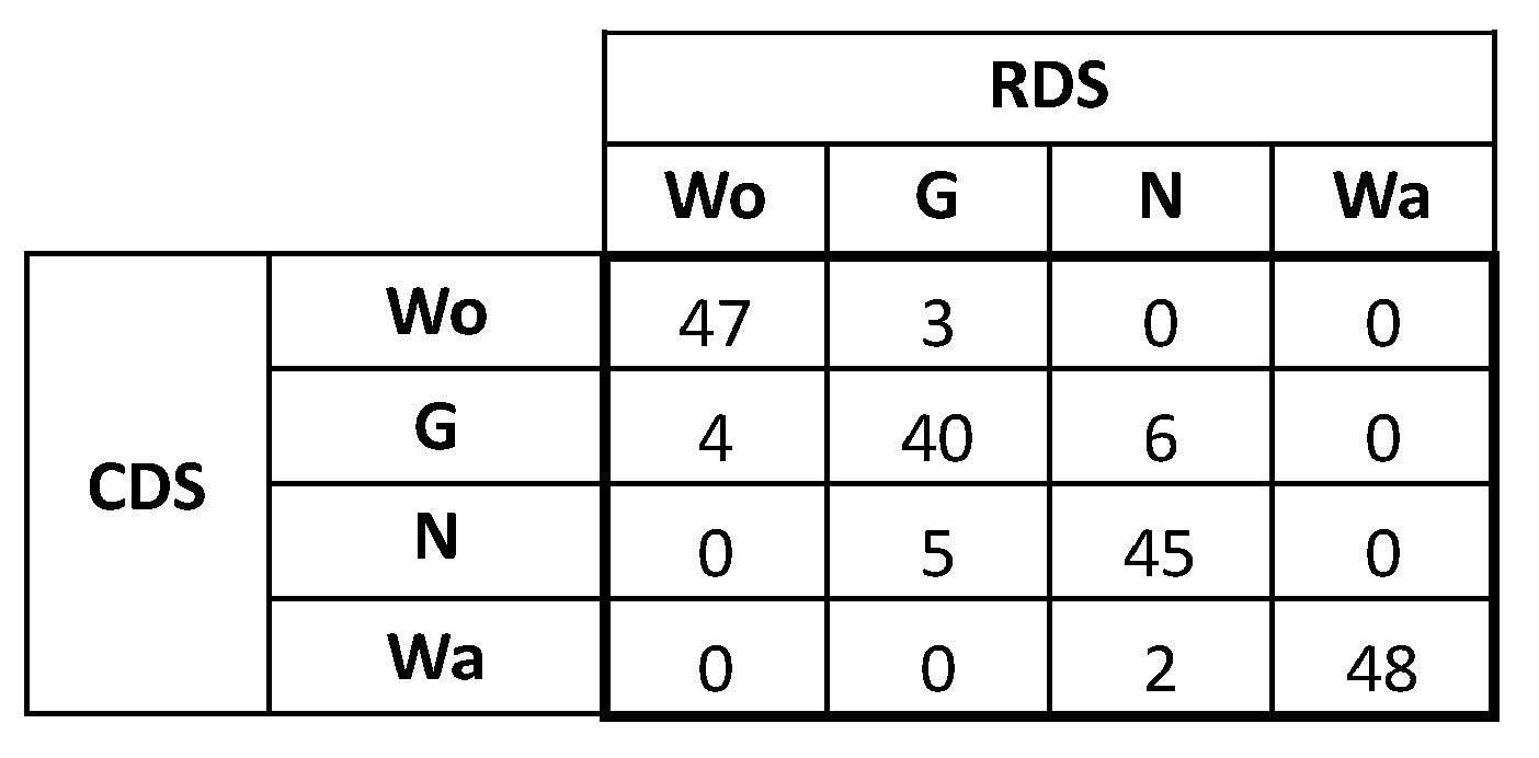
In order to illustrate the application of the above with an example, Figure 1 shows a confusion matrix from [37] with the results from the accuracy assessment of the classification of a synthetic data set with four categories. Now, let us consider that the RDS used in this assessment does have the quality to be a reference. Therefore, the data from Figure 1 cannot be understood as a complete multinomial but, rather, as a set of four multinomials, one for each category (column). 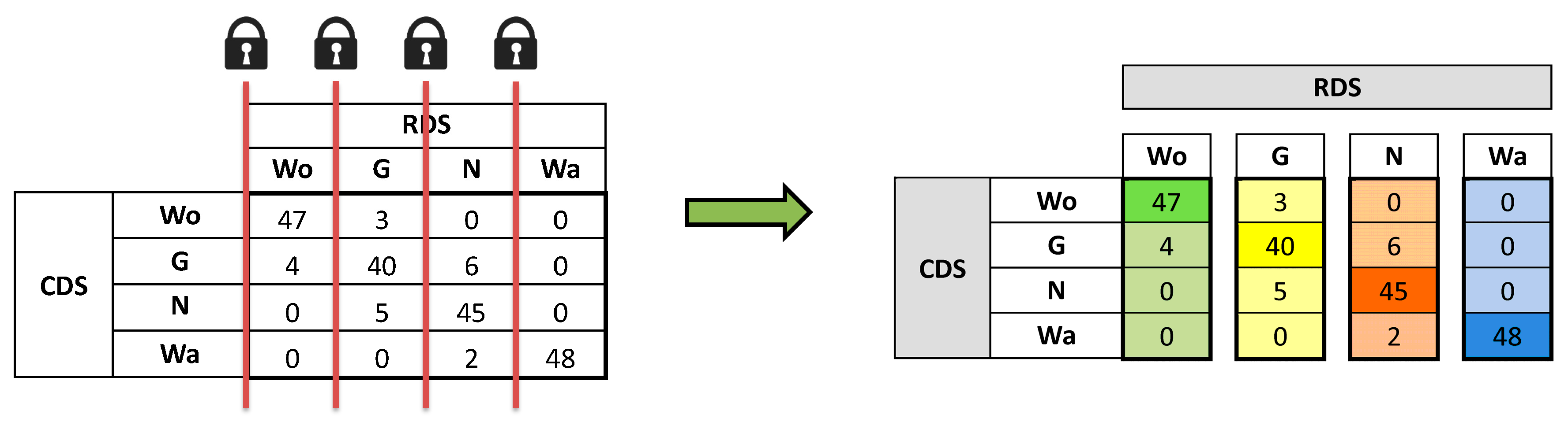Figure 2 illustrates this fact with locks that symbolize that the marginals of the columns are fixed and therefore, the new structure “quality control column set” (QCCS) has to be considered instead of the classical method based on the confusion matrix.

Following with the example, once the QCCS structure is considered, our proposal allows us to consider a set of quality specifications in the following manner: For each category, a classification level can be stated, but also a misclassification level with each other category (or groups of them). In

Table 1. Example of a set of specifications ¹: The quality levels required for each category and the percentage of misclassifications allowed between classes within each category.

Category	Specification ID	Description
Woodland	SpWo#1	95% of the minimum percentage required in well-classified items (≥95%)
	SpWo#2	4% of the maximum percentage allowed in misclassifications with Grassland (≤4%)
	SpWo#3	1% of the maximum percentage allowed in misclassifications with both Non-vegetated and Water (≤1%)
Grassland	SpG#1	88% of the minimum percentage required in well-classified items (≥88%)
	SpG#2	10% of the maximum percentage allowed in misclassifications with Non-vegetated (≤10%)
	SpG#3	2% of the maximum percentage allowed in misclassifications with both Woodland and Water (≤2%)
Non-vegetated	SpN#1	90% of the minimum percentage required in well-classified items (≥90%)
	SpN#2	8% of the maximum percentage allowed in misclassifications with Grassland (≤8%)
	SpN#3	2% of the maximum percentage allowed in misclassifications with both Woodland and Water (≤2%)
Water	SpWa#1	99% of the minimum percentage required in well-classified items (≥99%)
	SpWa#2	1% of the maximum percentage allowed in misclassifications with the other categories (≤1%)

¹ These specifications are only examples.

, we summarize an example of quality specifications that are supposed for the synthetic data presented in [37]. We indicate, for each category, the minimum percentage required for well-classified items, but also the maximum percentage allowed in misclassifications. As can be seen, we assume high percentages of well-classified items (≥95%, ≥88%, ≥90%, and ≥99%), low percentages in some misclassifications (≤4%, ≤10%, and ≤8%) and some other almost non-existent misclassifications (≤1% and ≤2%). Several misclassification levels group two or more categories. This possibility of merging categories offers a more flexible quality control analysis. For example, in Table 1, it is indifferent to the expert that the water is misclassified with any of the remaining three classes, but in relation to the Grassland class, the expert is more worried about a misclassification with Woodland or Water (≤2%) than a misclassification with Non-vegetated (≤8%).

As will be seen in later sections, our proposal of an exact multinomial test requires an order in the probabilities. Therefore, the set of quality specifications of Table 1 is not complete until we state, for each category, which order is assumed for them. For our example, we assume the order in which specifications are presented in Table 1. That is to say, for the category Woodland, the specification SPWo#1 is the most important one to be fulfilled, the second is SpWo#2, and finally, the third is SpWo#3, but any other order could have been considered.

3. QCCS Statistical Basis

The core of this section is twofold: (i) we introduce the QCCS structure starting from the confusion matrix and point out the implications of RDS as a reference for dealing with the data from a statistical point of view, and (ii) we state the quality levels required for the classification and determine when we will decide whether such quality levels are achieved or not by means of an exact multinomial test.

3.1. From the Confusion Matrix to the Set of Multinomial Distributions

Let ${\mathsf{\Gamma }}_1,\dots , {\mathsf{\Gamma }}_k$ be the $k$ true categories of the RDS and $G_1,\dots , G_k$ be the categories of the CDS, assigned by the classification process. Adscription of an item into the cell $\left(i,j\right)$ implies that it belongs to category $j$ in the RDS, and, by the classification procedure, it is classified as corresponding to category $i$ in the CDS. So, the elements inside the cells $\left(i,j\right), i=j$ are correctly classified, whereas an assignation into the cell $\left(i,j\right), i\ne j$ implies an error or misclassification. Finally, $n_{ij}$ indicates the number of items assigned to the cell $\left(i,j\right)$, and $n_{+j}$ is the sum of items that belong to the true category ${\mathsf{\Gamma }}_j, j=1,\dots ,k$.

Table 2. Notation of a $k\times k$ cross-classification. CDS: controlled data set; RDS: reference data set.

		RDS
		${\mathsf{\Gamma }}_1$	${\mathsf{\Gamma }}_2$	$\dots$	${\mathsf{\Gamma }}_{\mathit{k}}$
CDS	${\mathit{G}}_{\mathbf{1}}$	$n_{11}$	$n_{12}$	$\dots$	$n_{1k}$
	${\mathit{G}}_{\mathbf{2}}$	$n_{21}$	$n_{22}$	$\dots$	$n_{2k}$
	$⋮$	$⋮$	$⋮$	$⋮$	$⋮$
	${\mathit{G}}_{\mathit{k}}$	$n_{k1}$	$n_{k2}$	$\dots$	$n_{kk}$
Total		$n_{+1}$	$n_{+2}$		$n_{+k}$

displays the disposition of classification results corresponding to a $k\times k$ cross-classification.

If we consider the independence and randomness in the sampling procedure, the first approach is to see the whole matrix as one realization of a multinomial distribution. Recall that the multinomial distribution arises from an extension of the binomial distribution to situations where each trial has more than two possible outcomes. In a classical confusion matrix, the vector of possible success is one obtained from the cross-classification derived from the classification procedure. To be rigorous, if we realize $n$ independent trials where we carry out the cross-classification of an item in one of $c=k\times k$ cells, we define $X_i, i=1,\dots ,c$ as the number of times that the outcome associated with cell i occurs after reordering the matrix by columns to construct a vector. So, the vector $X=\left(X_1,X_2,\dots ,X_c\right)$ is said to have a multinomial distribution with parameter $n$, the number of trials, and the probability vector $\pi =\left( {\pi }_1, \dots ,{\pi }_c\right)$, with each ${\pi }_i\ge 0$ corresponding to the occurrence probability of the classification results in each cell, satisfying ${\displaystyle \sum }_{i=1}^c{\pi }_i=1$, in short,$M\left(n,\pi \right)$. Hence, the mass probability function of this distribution $M\left(n,\pi \right)$ is given by

$$P[\left(X_1=n_1, \dots ,X_c=n_c\right)= \frac{n!}{n_1!\dots n_c!}{\pi }_1^{n_1}\dots {\pi }_c^{n_c},$$

(2)

where ${\displaystyle \sum }_{i=1}^c{n}_i=n$.

However, if the RDS has the quality to be a reference, not all possible values of this multinomial are feasible. Next, we point out two situations as illustrative examples:

• For any category ${\mathsf{\Gamma }}_j$ (reference), there are $n_{+j}$ items in this column, so it is impossible to find a value $n_{ij}>n_{+j}$ in the same column. This could be possible only if RDS is not considered as a reference, that is, without constraints in the randomness of the matrix. In addition, the $n_{+j}$ elements can be correctly classified or confused with other categories, but they will always be located in the same column and never in other different columns (categories). This implies that the inherent randomness of the multinomial is not possible now.
• According to Equation (2), a possible outcome of an $M\left(n,\pi \right)$ can concentrate all items in one cell, say $\left(n,0,\dots ,0\right)$, but if RDS is considered to be a reference, this outcome will never be observed, because the values $n_{+j}$ are always present and, in consequence, all outcomes are partially grouped into subsets that sum $n_{+j}$.

Therefore, as stated in Section 2, when RDS is considered as a reference, the values $n_{+j}$ are fixed, and by redefining the outcomes for this number of trials, we can obtain a new multinomial distribution, one for each category.

So, we take advantage of this fact and we propose to deal with the information contained in Figure 1 as the new structure called the “quality control column set” (QCCS) (Figure 2) in order to differentiate it from the classical confusion matrix concept. Now, each column in the QCCS structure can be modeled as a different multinomial distribution. Moreover, a column can be modeled as a binomial distribution if a single misclassification level is set for all other (k − 1) categories in the specifications (e.g., specification SpWa#2 in Table 1).

The main advantage of this approach is that it allows us to assume specific quality requirements for each class analyzed and to test them. Now, we can propose a category-wise control method that allows us to establish levels of quality, category by category (column by column), related to the percentage of correctness in the classification for a particular class and to the percentage of possible misclassifications or confusions between classes. So, for each category and in a separate way, we can state a set of quality specifications, and in order to test whether such specifications are achieved or not, we propose an exact multinomial test.

3.2. Thematic Accuracy Quality Control

In order to fix the terms to be used, for a particular category Γ, we call the class that gives its name the “main class”, and the “rest of classes” are the remaining initial classes in the confusion matrix or new ones after the merging of one or more initial classes.

We have to put the rest of the classes in an assumed order, which we can establish freely. As an example, we come back to Table 1. In the quality requirements for the Grassland category, the main class is Grassland and, as stated at the end of Section 2, a confusion with Non-vegetated is considered more important than a confusion with both Woodland and Water. Therefore, the second class is Non-vegetated, and the third class is the new class Woodland + Water. So, we work with a multinomial distribution with three classes, $X=\left(X_1,X_2,X_3\right)$ where $X_1$ represents the number of items in the main class that are correctly classified, $X_2$ counts the number of confusions between the main class and the second class, and $X_3$ stands for the number of misclassifications between the main class and the third class.

According to the previous notation, quality control involves establishing the following quality conditions for each category:

• The minimum proportion of well-classified items in the main class;
• The maximum possible $k-1$ misclassification proportions between the main class and the rest of the classes.

At this point, we have to define when the classification results of a category agree with the specifications given previously. The criteria adopted are that the specifications are not fulfilled when:

• The number of correct items in the main class is lower than those expected, or
• If the number of correct items in the main class is equal to those expected, the number of misclassifications with the second class is greater than the expected, or
• If the number of correct items and the number of misclassifications with the second class is equal to those expected, the number of misclassifications with the third class is greater than that expected, and so on.

As a consequence, thematic accuracy quality control implies the proposal of a test for testing the following null hypothesis:

ℍ₀: The classification results agree with the set of specifications stated in the quality control for each category.

(3)

Assuming the QCCS is an independent set of $k$ multinomial distributions, we can propose 1, 2, or even $k$ different null hypotheses (one for each category/column), and hence, we can perform up to k independent tests. In the case of desiring a global hypothesis test, the Bonferroni correction is used. Therefore, this approach allows a more flexible way of understanding and testing thematic accuracy quality control than the classical methods based on the confusion matrix.

3.3. The Exact Multinomial Test

From now on, in order to maintain the notation as simple as possible, we are going to test the null hypothesis of Equation (3) for a fixed category, say Γ, that will represent any of the set $\left\{{\mathsf{\Gamma }}_1,{\mathsf{\Gamma }}_2,\dots ,{\mathsf{\Gamma }}_k\right\}$, and hence we will test whether the thematic quality specifications previously stated are achieved or not in the sense of the null hypothesis ${ℍ}_0$.

Thus, we consider that for a particular category Γ, we have $m$ elements to classify (which corresponds to its marginal value in Table 2), and we define $X_1$ as the number of elements correctly classified in the main class Γ, and we define $X_i,i=2,\dots ,q$, $q\le k$ as the number of misclassifications between the main class and the rest of the classes in decreasing order, assumed in the misclassification levels. In this way, we obtain a multinomial vector $X=\left(X_1,X_2,\dots ,X_q\right)$ with the parameter $m$ and the probability vector $p_0=\left(p_{10},p_{20},\dots ,p_{q0}\right), p_{i0}\ge 0, {\displaystyle \sum }_{i=1}^q{p}_{i0}=1$, with $p_{10}\ge p_{20}\ge \dots \ge p_{q0}$, with $p_{i0}$ being the percentage stated in the limits expressed in a set of specifications (e.g., Table 1) under the null hypothesis.

To test Equation (3), an exact test is proposed. Remember that an exact test calculates the empirical probability of obtaining an outcome as different from the null hypothesis as to the outcome observed in the data. So, the p-value is computed by adding up the probabilities of feasible outcomes in $M\left(m,p_0\right)$ (say, $P\left[X=x\right]$) under the alternative hypothesis, starting from the observed classification results. To decide when a classification result $X=\left(x_1,x_2,\dots ,x_q\right)$ is worse than $Y=\left(y_1,y_2,\dots ,y_q\right)$ according to the specifications (denoted by $X{<}_{m}Y$), we consider the following partial order relation between $X$ and $Y$ in the set $\left\{x_1,x_2,\dots ,x_q\in \left\{0,1,\dots ,m\right\}: {\displaystyle \sum }_{i=1}^q{x}_i=m\right\}$, which is similar to the lexicographic order, in the following sense,

$$\begin{array}{c}X{<}_{m}Y\mathrm{if}(x_1<y_1)\vee \\ \{(x_1=y_1)\wedge (x_2>y_2)\}\vee \\ \left\{\left(x_1=y_1\right)\wedge \left(x_2=y_2\right)\wedge \left(x_3>y_3\right)\right\}\dots \dots .\\ \left\{\left(x_1=y_1\right)\wedge \dots \wedge \left(x_{q-1}=y_{q-1}\right)\right\}\wedge \left(x_q>y_q\right),\end{array}$$

(4)

where $\wedge$ and $\vee$ represent the basic operators of Boolean algebra “AND” and “OR”, respectively.

$X=\left(x_1,x_2,\dots ,x_q\right)$ is equivalent to $Y=\left(y_1,y_2,\dots ,y_q\right)$ if $x_i=y_i,1\le i\le q$, (denoted by $X{=}_{m}Y$). So, given the observed classification, say $Y^{*}=\left(y_1^{*},y_2^{*},\dots ,y_q^{*}\right)$, the p-value is obtained as:

$$p={\displaystyle \sum }_{X{\le }_{m}Y*}{P}_0\left[X=x\right]$$

(5)

where $P_0\left[X=x\right]$ denotes the probability mass function under the null hypothesis, $M\left(m,p_0\right)$. In Appendix A, a detailed calculation of the exact p-value is included.

This technique has been previously used for inference purposes involving multinomials. For instance, for the positional accuracy quality control of spatial data in [38,39] and in general for testing problems in contingency tables ([40,41], among others).

Once the p-value is calculated, the rule set is:

• For a single column, the null hypothesis in Equation (3) should be rejected if the $p$-value obtained is less than the nominal value α.
• For L categories/columns, $2\le L\le k$, we calculate the corresponding $p$-values for each testing problem. Assuming independence between the tests, we can state the global hypothesis of the quality requirements. To assure that the global size of the type I error is less than or equal to α, the Bonferroni criteria are used [42]. As a consequence, we should reject the global null hypothesis if at least one $p$-value is less than or equal to $\alpha /L$.

As mentioned before, for each column of the QCCS, a different multinomial distribution can be proposed in the null hypothesis. This fact implies dealing with a set of multinomial distributions with equal or different amounts of classes (dimension) and equal or different levels in the quality requirement (probability vector). Binomial distributions are considered if all misclassification levels are merged to a single value.

4. Application

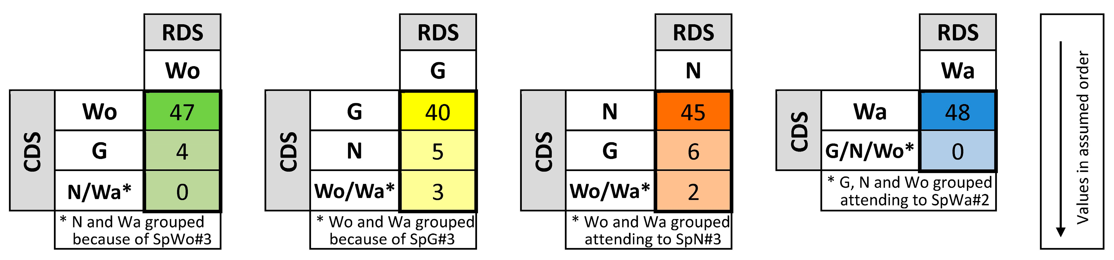
The data in Figure 2 and Table 1 are used to illustrate how this new structure QCCS works and how the exact tests are used for testing whether the levels of thematic accuracy are achieved or not. Figure 3 summarizes the specifications from Table 1 regarding the percentage of correctness and the limits on the misclassifications for each category. It presents the set of probability vectors, each one with values in the assumed order, and also groups some categories if the specifications do not analyze them separately. Figure 4 shows the same data as Figure 2, but the values in each column are ordered and grouped following Figure 3.

The required assumptions for these tests are as follows:

• The positional accuracy is adequate for the scale of the thematic product;
• The RDS is an adequate quality reference for this new approach of thematic accuracy quality control.

Assuming the set of specifications presented in Table 1 (Figure 3), we define the corresponding null hypotheses for each column, and we illustrate the application of this new approach to this example.

a. Woodland.

According to Figure 3 (column Wo), for the Woodland category, we define a multinomial distribution with three categories: $X_1$ denoting the number of elements correctly classified; $X_2$, the number of elements confused with Grassland; and $X_3$, the number of elements classified as Non-vegetated or Water. Therefore, $q=3$. The specifications lead us to the multinomial $M\left(51,p_0\right)$ with $p_0=\left(0.95, 0.04, 0.01\right)$.

In this case, the observed classification is $Y^{*}=\left(47, 4, 0\right)$ (see Figure 4, column Wo), and the p-value is obtained by adding up the probabilities of $M\left(51,p_0\right)$ for classification outcomes that are worse according to the partial order $\le { }_m$. The value obtained is 0.1678.

b. Grassland.

Along the same lines, from Figure 3 (column G), we define $X=\left(X_1,X_2,X_3\right)$, with $X_1$ being the number of elements correctly classified, $X_2$ being the number of misclassifications with Non-vegetated, and $X_3$ being the number of misclassifications with Woodland or Water. $X$ follows $M\left(48,p_0\right)$ with a probability vector of $p_0=\left(0.88, 0.10, 0.02\right)$.

The observed classification is $Y^{*}=\left(40,5,3\right)$ (see Figure 4, column G), and the p-value obtained is 0.2229.

c. Non-vegetated.

Following similar reasoning to that used in the previous categories, the multinomial distribution is $M\left(53,p_0\right)$ with $p_0=\left(0.90, 0.08, 0.02\right)$, defined from the specifications shown in Figure 3 (column N).

The observed classification is $Y^{*}=\left(45, 6, 2\right)$ (see Figure 4, column N), and the p-value obtained is 0.1785.

d. Water.

In this category, as expressed in Table 1 and Figure 3 (column Wa), the maximum percentage of misclassified elements is 1%, so the classification results lead us to define a binomial distribution with the following parameters: the number of elements to be classified, $m=48$, and the probability of correctness in the classification, $p=0.99$, in short, $B\left(48,0.99\right)$.

The observed classification is $Y^{*}=48$ (see Figure 4, column Wa), and the p-value obtained is 1.

Overall decision. For this QCCS, four hypothesis tests were carried out, and in order to assure the same significance level, $\alpha =0.05$, we applied the Bonferroni correction to compensate for the number of tests. As a consequence, we reject the hypothesis that the thematic quality levels specified in Table 1 and Figure 3 are globally achieved if any of the four p-values obtained are less than $\alpha /4=0.0125$. It does not occur in this example, and we can conclude that the data shown in Figure 4 globally satisfy the quality conditions stated in Table 1 (Figure 3). In addition, the individual analysis of each testing problem concludes that all of the quality requirements considered are accomplished.

In this example, we have illustrated how the QCCS can be applied and how it offers a more flexible and complete way to test statistically when a set of quality criteria are fulfilled, from both individual and global points of view. Such a detailed analysis would not be possible with the classical methods based on the confusion matrix.

5. Conclusions

In this study, a new approach for thematic accuracy quality control was presented. The approach is based on the assumption that the RDS does have the quality to be a reference, and this fact makes a more powerful and complete method for thematic accuracy quality control available than those based on a confusion matrix or on global indices. This method allows class by class quality control, which can consider not only the percentage of correctness but also the degree of misclassifications or confusion with other classes. It is a very flexible procedure because it allows us to simultaneously test the quality levels for a set of categories, and it also provides the possibility to merge classes when considering the misclassifications, which means the possibility of varying the dimensions of the underlying multinomial.

The proposed exact multinomial test for a category is based on a criterion for the achievement of the specifications. This criterion has been stated to be a partial order relation $X\le { }_{m}Y$ between classification results $X$ and specifications $Y$, which is similar to the lexicographic order. The procedure follows the same steps if the user changes the definition of $X{\le }_{m}Y$ and, as a consequence, the calculation of the p-value of the corresponding testing hypothesis.

If a global hypothesis test is desired for L categories, the Bonferroni criteria are proposed. As a consequence, we should reject the global null hypothesis if at least one $p$-value is less than or equal to $\alpha /L$.

The new approach can be widely applied to thematic accuracy quality control of any kind of spatial data in which the classification correctness should be assessed.