An Improved MB-LBP Defect Recognition Approach for the Surface of Steel Plates

Abstract

The detection of surface defects is very important for the quality improvement of steel plates. In actual production, as the steel plate production line runs faster, the steel surface defect detection algorithm is required to meet the requirements of real-time detection (less than 100 ms/image), and the detection accuracy is improved (at least 90%). In this paper, an improved multi-block local binary pattern (LBP) algorithm is proposed. This algorithm not only has the simplicity and efficiency of the LBP algorithm, but also finds a suitable scale to describe the defect features by changing the block sizes, thus ensuring high recognition accuracy. The experiment proves that the method satisfies the requirements of online real-time detection in terms of speed (63 ms/image), and surpasses the widely-used scale invariant feature transform (SIFT), speeded up robust features (SURF), gray-level co-occurrence matrix (GLCM), and LBP algorithms in recognition accuracy (94.30%), which prove that the MB-LBP has practical application value in an online real-time detection system.

1. Introduction

Steel plates are widely used in engineering fields such as ships, bridges, machinery, construction, and automobile manufacturing. In the production process of a plate, due to the rolling process, various types of defects are easily formed on the surface of steel plates such as cracks, scratches, indentations, pits and scales [1]. These defects have a great impact on the appearance and performance of the product, so it is extremely important to detect the surface defects on the plate.

The surface defect recognition algorithm for steel plates is the core part of the entire surface defect detection system. Yun et al. [2] proposed a new defect detection algorithm, which is based on Gabor filters. The Gabor filters are optimized using a new optimization algorithm known as the univariate dynamic encoding algorithm for searches. The algorithm finds the minimum value of the cost function related to the energy separation criteria between the defect and the defect-free regions. Xu et al. [3] proposed a classifier based on Ads Boosting algorithms for the classification of defects with textural features that employed non-sampling wavelet decomposition to the scale co-occurrence matrix of the low-pass component and the grayscale co-occurrence matrix of the high-pass component. Pan et al. [4] proposed an engineering-driven rule-based detection (ERD) method. The ERD consists of three detection stages using the pixel features of bleeds, which are transferred from the physical features generated via engineering knowledge. Yu et al. [5] proposed a surface trait extraction method based on complex Contourlet decomposition, which has the characteristics of shift invariance, excellent directional selectivity, and a higher retrieval rate. Industrial test results show that the accurate rate of classifying surface features is about 90%, and it can be used in image feature extraction and slab defect detection. Miyamoto et al. [6] proposed a one-shot measurement using the plane-wave with the time-of-flight (TOF) based transmission method and validated the method using wave propagation simulations. The defect in billets can be detected regardless of the defect position even in the vicinity of the surfaces of a billet. Yan et al. [7] proposed a mathematical morphology detection method based on multi-scale element, which can not only filter the noise effectively, but can also delete the false characteristics of the cracks, scales, and slag. Lin et al. [8] proposed a robust detection method based on the vision attention mechanism and deep learning of feature map in order to relieve the problem of the false and missed detection of casting defects in x-ray detection. The experimental results showed that the false rate and missed rate for the detection of casting defects were less than 4%, and the accuracy of the defect detection was more than 96%. Di et al. [9] proposed a new semi-supervised learning method based on convolutional auto encoder (CAE) and semi-supervised generative adversarial networks (SGAN) to classify the surface defects of steels. Jiang et al. [10] suggested a method for detecting the appearance defect of castings based on a deep residual network. This method divides the casting into multiple regions, preprocesses the image of each region, and then inputs the processed image into the convolutional neural network to extract the features, before finally determining whether the sample has defects.

All of the above methods effectively solve the problem of recognition accuracy. However, in actual production, the steel production line runs very fast, so the surface defect detection algorithm needs to meet the real-time requirements while ensuring the accuracy.

In this paper, we propose the multi-block local binary pattern (MB-LBP) algorithm to extract the features of the surface defects of steel plates. The experimental results show that the MB-LBP algorithm meets the requirements of the online detection of steel plate defects in terms of both speed and accuracy.

The rest of this paper is organized as follows. Section 2 introduces the surface defects of steel plates. Section 3 introduces the principle of MB-LBP. Section 4 introduces the experiments and analysis of surface defect detection based on MB-LBP. Finally, the conclusions are discussed in Section 5.

2. Surface Defects of Steel Plates

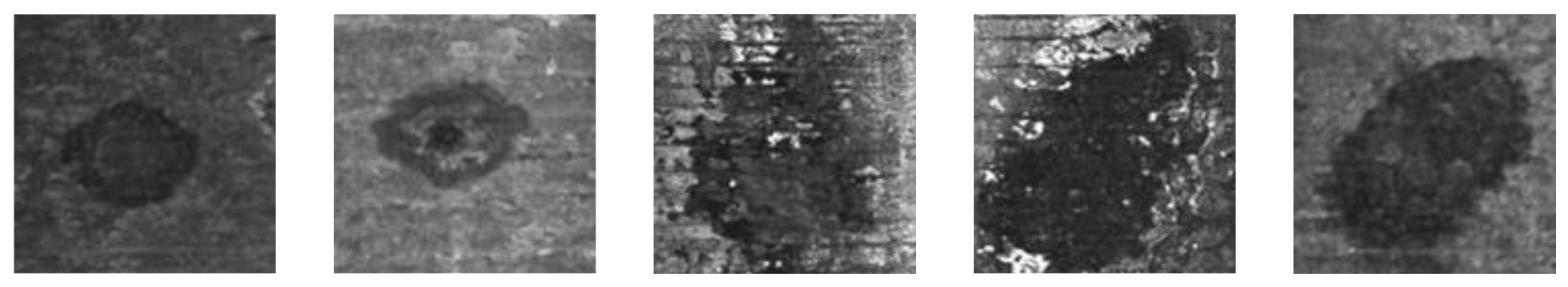
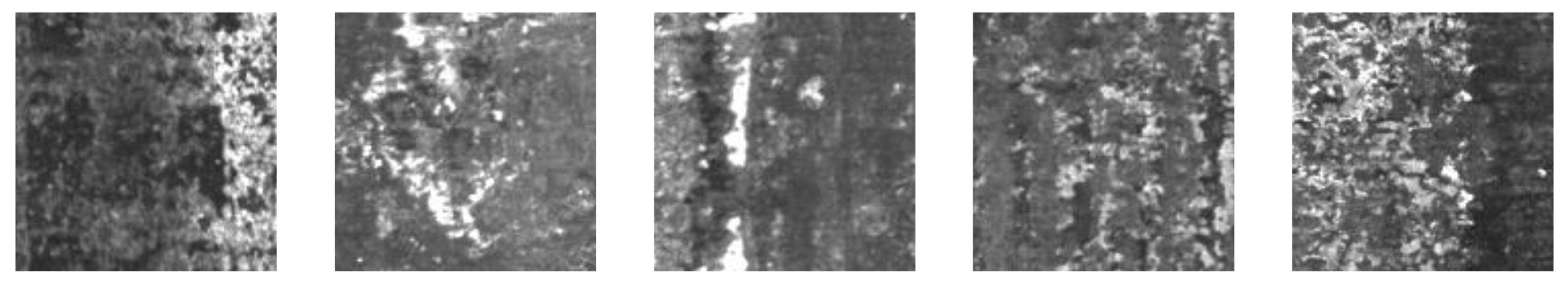
Based on our observations and research, the surface defects of slabs can be divided into five types: cracks, scratches, indentations, pits, and scales. The following are several common defect samples collected from the surface defect online detection system.

2.1. Cracks

Cracks are the most serious defect on the surface of steel plates, as shown in Figure 1. Cracks may cause tremendous damage in the following rolling procedure [11].

2.2. Scratches

Scratches are generally due to friction between the mechanical equipment or the relative motion of the plates on the roller table [12]. Scratches mostly appear as bright stripes in the image, as shown in Figure 2. Since scratches are mostly caused by mechanical equipment, they appear periodically at most times. That is, scratches appear continually in adjacent images, and their positions and features are similar, so scratches are easier to classify.

2.3. Indentations

The occurrence of indentations is due to inclusions in the plates during continuous casting, and pits appear on the surface of the billet, or as depressions on the surface of the roller table. The typical images of indentation are shown in Figure 3. Casting temperature, improper control of casting speed, entrapment of protective slag, etc., can cause defects on the surface and inside of the strand, especially surface flaws, pits, and buckling defects. During the heating and rolling process, it is possible to further form an indentation. The indentation seriously affects the quality of the casting blank as the indentation size varies, the direction is uncertain, and the manual inspection is difficult.

2.4. Pits

Pits are pit-shaped defects with a certain depth due to the periodical vibration of the mold during the production of the plates. Typical images of a pit are shown in Figure 4. The pits easily cause indentations during the subsequent hot rolling process, which is one of the important factors affecting the surface quality of the plates. In addition, cracks may occur at the bottom of deep pits. Pits are common on the surfaces of the plates. Shallow pits have little effect on the surface quality of the plates, but deeper pits require more attention.

2.5. Scales

The surface temperature of the continuous plates during production is usually around 1000 °C, so the surface is easily oxidized to form oxide scales. The typical images of scales are shown in Figure 5. Scales do not seriously affect the quality of the plate, but they have a great negative effect on the recognition of the surface defects of the plates.

3. Principle of Multi-Block Local Binary Pattern

3.1. Principle of Local Binary Pattern

Due to the high ambient temperature and complex image background, the detection of surface defects for steel plates becomes a puzzling problem. The change of illumination will cause a linear change in the gray level of the image. The local binary pattern (LBP) is a method to describe the texture of the image that can eliminate linear illumination by comparing the gray values of pixels. LBP was introduced by Ojala [13,14] and has been widely applied in many fields [15] such as metal surface quality detection [16], paper quality detection [17], image texture analysis [18], and target detection [19].

The LBP descriptor was initially proposed as an effective grayscale-invariant texture descriptor based on image gray levels. The basic LBP descriptor is defined in a 3 × 3 pixel area. The gray value of the center pixel is s $g_c$. The gray values of its 8 neighborhood pixels are $g_0$...$g_7$, respectively. The texture description T of the center pixel can be expressed as Equation (1):

$$\mathrm{T}~\left(g_0-g_c,\cdots ,g_7-g_c\right)$$

(1)

Then, compare the gray values of the eight neighborhood pixels with $g_c$. If the value is greater than $g_c$, the binarization value of the pixel is 1, otherwise the binarization value of the pixel is 0. Then, the texture description T after binarization can be expressed as Equation (2).

$$\mathrm{T}~\left(s(g_0-g_c\right),\cdots ,\mathrm{s}\left(g_7-g_c\right))$$

(2)

s(x) is calculated by Equation (3):

$$\mathrm{s}\left(\mathrm{x}\right)=\{\begin{array}{c}1,x>0\\ 0,x\ll 0\end{array}$$

(3)

After binarization, randomly choose one of eight neighborhood pixels as a starting point. It is worth noting that the choice of starting point is random, but the choice of starting point for the entire image should be consistent, for convenience, this paper consistently selected the top left point as the starting point. Then, encode all binarization values clockwise to a binary number. Therefore, the LBP value of pixel $\left(x_c,y_c\right)$ is calculated in Equation (4).

$$\mathrm{LBP}\left(x_c,y_c\right)={\displaystyle \sum }_{i=0}^{7}s\left(g_i-g_c\right)2^i$$

(4)

Figure 6 shows the complete process of the local binary pattern (LBP).

The LBP value for each pixel could be calculated by the above calculation process. In this way, an LBP image can be obtained [20].

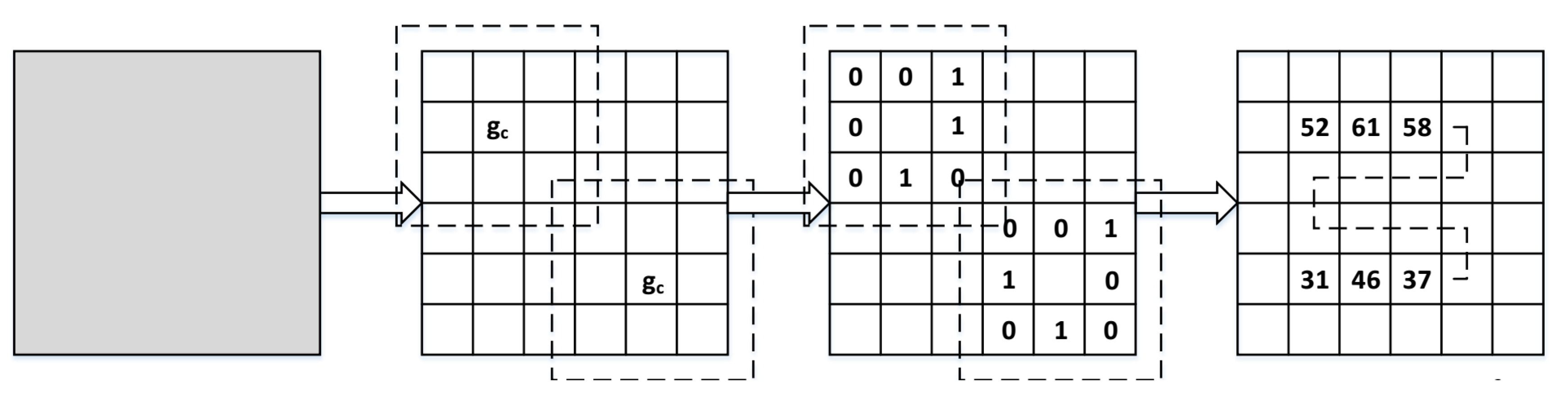
3.2. Principle of MB-LBP

A series of improved LBP algorithms have been proposed such as the LBP uniform pattern and LBP rotation-invariant pattern. All of these LBP algorithms are always focused on a single point. However, different defects have different sizes, and the appropriate scale to describe their texture features is different (larger defects should be described by more points), so different block sizes (with different number of points) should be selected. Therefore, this paper proposed the multi-block LBP (MB-LBP) to describe features of various defects with different sizes [21].

The specific steps of the MB-LBP are as follows:

(1) Division:

The source image is divided into small blocks, and each block contains n × n pixels (take 2 × 2 as an example).

(2) Binarization:

Calculate the mean gray value of all blocks, then compare the mean gray value of each block with the mean gray value of its neighborhood block. If the mean gray value of the neighborhood block is 50% larger than the center block, then set it as 1, otherwise set it as 0, as shown in Equation (5):

$$s\left(g_i,g_c\right)=\{\begin{array}{c}1,\frac{\left|g_i-g_c\right|}{g_c} >50\%\\ 0,\frac{\left|g_i-g_c\right|}{g_c} \le 50\%\end{array}$$

(5)

where $g_i$ is the mean gray value of each neighborhood block and $g_c$ is the mean gray value of the center block.

Another improvement of the MB-LBP to LBP is that, when calculating $s\left(g_i,g_c\right)$, it no longer simply compares the mean value of the neighborhood block with the center block, but compares the percentage of the difference of the mean value with the center block. Therefore, the robustness of the MB-LBP can be enhanced.

The binarization process is shown in Figure 7.

(3) Computation of MB-LBP pattern value:

First, randomly choose one of the eight neighborhood blocks as a starting point. It is worth noting that the choice of starting point is random, but the choice of starting point for the entire image should be consistent, for convenience, this paper consistently chose the top left point as the starting point.

Then, encode all binarization values clockwise to a binary number as calculated by Equation (6)

$$\mathrm{MB}-{\mathrm{LBP}}_P^R\left(x_c,y_c\right)={\displaystyle \sum }_{p=0}^{p-1}s\left(g_i,g_c\right)2^p$$

(6)

(4) Get MB-LBP pattern value of entire image:

Calculate the MB-LBP pattern value of each block traversing the entire image, from left to right, top to bottom. For the edge block, its neighborhood block is missing, and it has little effect on the texture feature of defects located inside the image, so THE MB-LBP pattern value of the edge block is ignored.

In this way, an entire MB-LBP image can be obtained, as shown in Figure 8.

4. Experiment and Analysis of Surface Defects Detection Based on MB-LBP

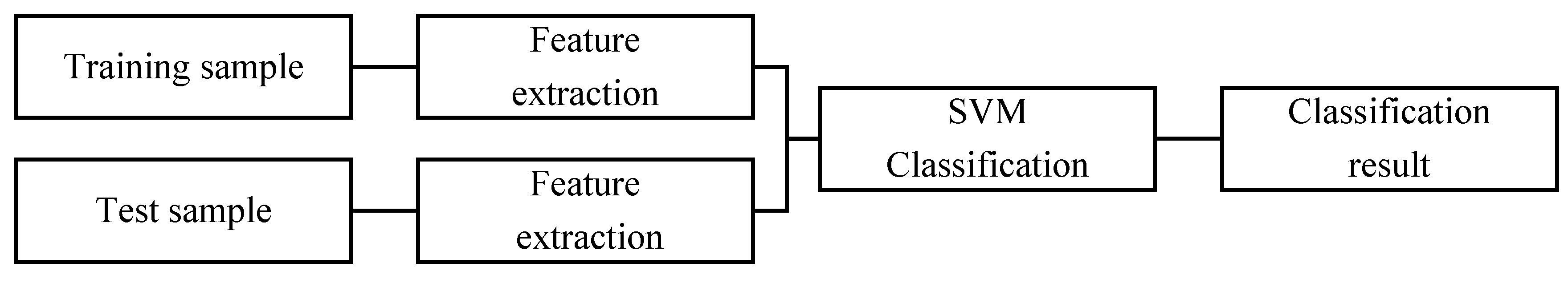
4.1. Experimental Design

4.1.1. Architecture of Surface Defect Detection System

A complete online surface defect detection system for steel plates should include image capturing, image preprocessing, defect feature extraction, and defect classification [22], which is shown in Figure 9. In pre-processing, the image segmentation algorithm is used to mark suspected defect areas. It can not only make preparations for identifying the sizes and locations of defects, but can also greatly reduce the amount of calculation for defect feature extraction and defect classification and identification. After the defect areas are determined, the defect features are extracted by the feature extraction algorithm. Then, the obtained feature vectors will be input into the classifier for classification and identification. Finally, a series of information such as class, size, location, and severity of the defect can be obtained.

4.1.2. Algorithms of Image Segmentation in Image Preprocessing

The steps of image segmentation in image preprocessing is as follows:

(1) Integral image segmentation.

The concept of integral images was proposed by Viola and Jones [23]. With the integral image, the grayscale sum of pixels in a rectangular area can be quickly calculated, which represents the features of this area. The value of any point in the integral image is the grayscale sum of all pixels from the upper left corner to this point, that is:

$$p(i,j)={\displaystyle \sum _{i\prime <=i\&j\prime <=j}pix(i\prime ,j\prime )}$$

(7)

where $pix(i,j)$ is the grayscale of the pixel located at $(i,j)$.

As shown in Figure 10, first, the original image is equally divided into blocks. The length and width of the block can be changed as a power of two (eight pixels in this paper). With the integral image, the mean grayscale of each block can be quickly calculated, which represents the features of this block.

(2) Differential calculation

Compare each block with four neighbor blocks and obtain all difference values. Then, select the difference value with the largest absolute value as the feature value of the current block. All feature values form a block difference matrix. The result is shown in Figure 11. The difference value in the block difference matrix reflects the change of the grayscale in the image. Blocks with a small difference value and gentle grayscale changes represent a no defect area; while blocks with a large difference value and sharp grayscale changes mean a suspected defect area.

(3) Threshold setting

Now, the question is how to select a reasonable threshold to determine whether the difference value is large or small. Set two thresholds, high and low, to divide the grayscale difference. As shown in Figure 12, the upper plane represents the high threshold and the lower plane represents the low threshold. The blocks with a difference value greater than the high threshold is identified as “master”, blocks with a difference value less than the low threshold is identified as “abort”, and blocks with a difference value between high and low threshold is identified as “candidate”. The “master” blocks are considered to be a defect area; the “candidate” block is a candidate defect area, and only when it has a “master” eight-neighbor block, will it be promoted to a ”master” block.

(4) Regional growth

Usually, a complete defect area is composed of multiple blocks. Therefore, it is necessary to merge adjacent “master” blocks into larger areas. That is, when there is a “master” block in eight-neighbor blocks of a “master” block, merge them as a new “master” block. Repeat the operations above until the new “master” block has no “master” block in its neighborhoods.

4.1.3. Experiment of Defect Feature Extraction and Defect Classification in this Paper

In this paper, MB-LBP was employed in feature extraction and support vector machine (SVM) was employed in the defect classification and identification.

The complete experiment process is shown in Figure 13.

The process of the MB-LBP + SVM experiment is detailed as follows:

(1) Image division

The image is divided into small blocks with n × n (n = 2, 4, 8, and so on) pixels, and then the mean gray value of the blocks are calculated as the gray value of the block.

(2) MB-LBP pattern value calculation

For each block, compare its gray value to each of its eight neighbors clockwise. When the gray value of center block is 50% greater than the gray value of neighbor block, write “0”. Otherwise, write “1”. This gives an 8-digit binary number, which is usually converted to decimals for convenience.

(3) Feature vector generation

Now, we have binary numbers of all blocks in the entire image. Then, compute the histogram of the frequency of each “binary number” occurring in the entire image.

An 8-digit binary number has 2⁸ = 256 different numbers at most. Therefore, this histogram can be seen as a 256-dimensional feature vector.

Such a large number of patterns will result in a long calculation time. Furthermore, a large pattern number will lead to a sparse feature vector that is difficult to compute. To solve these two problems, referring to the LBP uniform pattern [24], we proposed the MB-LBP uniform pattern. This idea is motivated by the fact that some binary patterns occur more commonly in texture images than in others [25]. These common binary patterns are called a uniform pattern if the binary pattern contains at most two 0–1 or 1–0 transitions. For example, 00010000 (two transitions) is a uniform pattern, 01010100 (six transitions) is not. Other uncommon binary patterns are called a non-uniformed pattern if it contains more than two transitions. The maximum MB-LBP uniform patterns is 59, much smaller than 256 of the original MB-LBP.

Figure 14 shows the comparison of the histogram between the original MB-LBP and MB-LBP uniform pattern.

(4) The generated feature vectors are sent to the SVM for classification and identification

The original SVM is a binary classifier. In this paper, the one-vs-one multi-classification SVM method [26] was adopted. Every two classes construct a SVM, and there are a total of n(n − 1)/2 SVM. The parameter n is the number of classes. In this paper, n = 5 and there were 5(5−1)/2 = 10 SVM in total.

The specific construction process is as follows:

(a)

Select two image classes, i and j in the training set as the positive and negative sample sets;

(b)

Extract the MB-LBP features of all images in class i and j, then represent all images by the histogram vector;

(c)

Train the classifier between class i and j;

(d)

Repeat steps (a)~(c) until the training between any two classes is completed. Obtain the optimal classification surface of all classifiers.

When a test image I is classified, vote to determine which class the image I belongs to according to the minimum sum of the distances from image I to the optimal classification surface.

4.1.4. Samples Sets of Experiment

The surface defect samples of the plates used in this paper were collected from a surface defect detection system in a steel company. The type composition of the sample sets is shown in

Table 1. Type composition of surface defect sample sets.

	Crack	Scratch	Indentation	Pit	Scale	total
Training	318	117	100	30	511	1076
Testing	296	175	174	139	913	1697

.

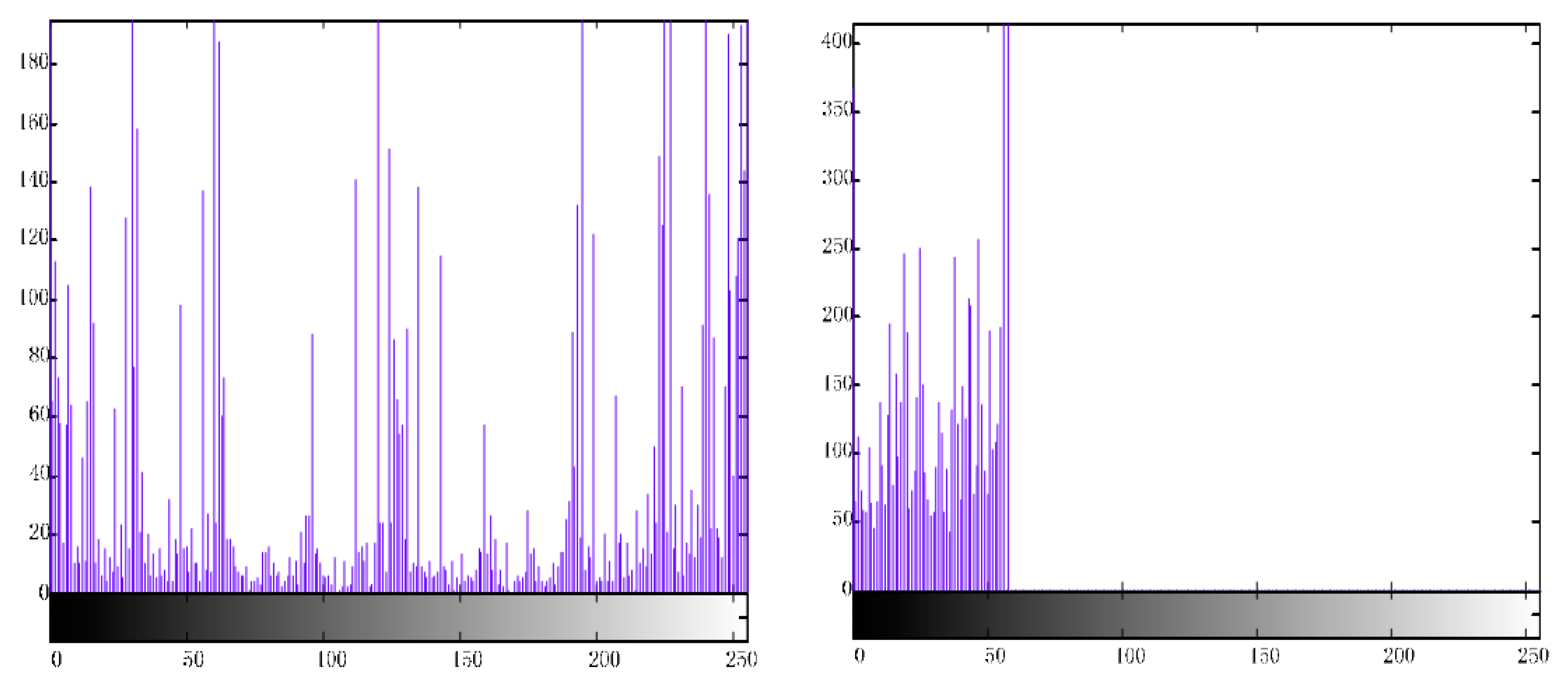
4.1.5. Parameter Selection of MB-LBP

There is a certain fluctuation in the recognition accuracy, as shown in Figure 15. When the block size increased from 2 × 2 to 4 × 4, the accuracy increased, and when it increased to 8 × 8, it decreased. This is because the block enlargement was equivalent to image compression, and too large a block size lost too much defect feature information, so the accuracy decreased. Through analysis, this experiment selected 4 × 4 block size for calculation.

4.1.6. Hardware Configuration of Experimental Platform

All algorithms were tested in the same platform. The hardware configuration was as follows: CPU Intel i5-490, main frequency 3.3 GHz, memory 8 GB.

4.2. Comparison of Experiment Result between MB-LBP and Other Algorithms

To validate the performance of the MB-LBP, a comparison with several other algorithms was made from the perspective of classification accuracy and time efficiency. The classification accuracy is the percentage of identified defects to the total defects. The time efficiency is the required time to compute the same size image on the same platform.

In this paper, the scale invariant feature transform (SIFT), the speeded up robust feature (SURF), the gray-level co-occurrence matrix (GLCM), and convolutional auto encoder-semi-supervised generative adversarial networks (CAE-SGAN) were selected for the comparison. The SIFT [27] algorithm is widely used in the fields of image matching, image recognition, and defect detection. It constructs a Gaussian scale space to describe the local features for the purpose of scale invariability, rotation invariability, and illumination invariability. This algorithm has a certain stability on overcoming the influence of noise and affine. The SURF [28] algorithm is improved based on the SIFT algorithm, which has not computed the Gaussian scale space. On the basis of retaining the main information of the feature points, SURF employs the box filtering technique to simulate the Gaussian scale space to improve the feature extraction speed. As a classic texture feature descriptor, GLCM [29] reflects the comprehensive information of a grayscale image with respect to direction, adjacent interval, and transform amplitude, and is the basis for analyzing the local pattern structure and arrangement rules of the images. The dimension of the feature vector extracted by GLCM is 256 × 256, hence the computation amount is too large. Aiming at this problem, the KLPP [30] was adopted to reduce the dimensions of the feature vector. CAE-SGAN [9] is a deep learning method based on convolutional auto encoder (CAE) and semi-supervised generative adversarial networks (SGAN). It first trains a stacked CAE through massive unlabeled data. After CAE is trained, the encoder network of CAE is reserved as the feature extractor and is fed into a softmax layer to form a new classifier. SGAN is introduced for semi-supervised learning to further improve the generalization ability of the new method. Same as the other deep learning methods, this method uses the original defect images as the network input.

The surface defect detection system for steel plates is an online real-time detection system, time efficiency is its key indicator. According to experience, for an online detection system, in order to ensure real-time requirements, the maximum time efficiency is 100 ms/image. On this basis, the recognition accuracy of the algorithm is as high as possible. For practicality, the accuracy should be at least 90%.

Table 2. Comparison of the recognition accuracy and time efficiency between the MB-LBP and other algorithms.

	Feature Dimension	Recognition Accuracy	Time Efficiency (ms/image)
SIFT	128	91.43%	583
SURF	128	86.89%	142
GLCM	20	84.27%	248
LBP	256	89.05%	41
MB-LBP	59	94.40%	63
CAE-SGAN	224 × 224 (original image)	96.21%	434

shows the comparison of the recognition accuracy and time efficiency between the MB-LBP and other algorithms. The time efficiency of SIFT, SURF, and GLCM speed was separately 583 ms, 142 ms, and 248 ms, which is too slow to meet the requirements of online real-time detection. The time efficiency of LBP was 41 ms, which not only meets the real-time requirements, but is also the fastest algorithm. However, its recognition accuracy was only 89.05%, lower than the minimum practical requirements. The time efficiency of MB-LBP was 63 ms. Although it was slightly slower than the LBP, it still meets the real-time requirement. Additionally, it had the highest recognition accuracy, reaching 94.40%. As for CAE-SGAN, as a deep learning method, it had the highest recognition accuracy of 96.21%. However, it uses the original image as input, and the dimension of input vector was as high as 224 × 224. Additionally, its network structure is too complicated. Therefore, its time efficiency was only 434 ms/image, much higher than the minimum requirement (less than 100 ms/image) of online real-time detection in this paper.

Table 3. Recognition accuracy of each class of defects with the MB-LBP.

Defects	Recognition Accuracy with MB-LBP
Crack	95.61%
Scratch	94.29%
Indentation	94.25%
Pit	95.68%
Scale	93.87%
Total	94.40%

shows the recognition accuracy of each class of defects with the MB-LBP. The recognition accuracy of all defects met the requirement of online detection (at least 90%). The recognition accuracy of most classes was above 94%, except for scales. This is because scales have complex morphological features and are difficult to classify. Recognition of scales is also one of the future improvement directions.

Figure 16 shows some examples of false matching. Cracks vary in size and shape, in particular, the detection of small cracks is difficult. Figure 16(a1,a2) show false-matching cracks, as they were too small and not obvious enough. Scratches were relatively easy to detect, but were greatly affected by light. Figure 16(b1,b2) show false-matching scratches. Figure 16(b1) was misclassified as a crack as it shows a thin dark stripe with weak light; and Figure 16(b2) was misclassified as a scale, as it shows an irregular area shape with strong light. Indentations vary in size and direction. Figure 16(c1,c2) show false-matching indentations. Two indentations with different sizes and directions were classified as different types of defects. Pits have irregularly shaped edges and complex backgrounds, like scales. Figure 16(d1,d2) show false-matching pits that were misclassified as scales. Scales have complex shapes and great grayscale changes, as such, they are the main misclassification defects. Scales have the lowest recognition accuracy, many other types of defects are misclassified as scales, or vice versa. Figure 16(e1,e2) show false-matching scales. Figure 16(e1,e2) were separately misclassified as a pit and crack due to their similar shapes.

5. Conclusions

Online detection of the surface defects of steel plates requires an algorithm that simultaneously satisfies fast recognition speed and high recognition accuracy.

In this paper, we proposed a surface defect detection algorithm for steel plates, which adopted the MB-LBP algorithm to extract the defect features. The MB-LBP algorithm divides the image into small blocks. After the binarization and MB-LBP value calculation, grayscale histograms were generated as the feature vectors of the image.

To verify the performance of the MB-LBP algorithm, a comparison with several other algorithms was made. The experimental results show that the recognition accuracy of the MB-LBP algorithm was better than the other algorithms, and the time efficiency was fast enough to meet the real-time requirements of the online surface defect detection of steel plates.

References

1. Suresh, B.R.; Fundakowski, R.A.; Levitt, T.S.; Overland, J.E. A real-time automated visual inspection system for hot steel slabs. IEEE Trans. Pattern Anal. Mach. Intell. 1983, PAMI–5, 563–572. [Google Scholar] [CrossRef]
2. Yun, J.P.; Choi, S.H.; Kim, J.W.; Kim, S.W. Automatic detection of cracks in raw steel block using Gabor filter optimized by univariate dynamic encoding algorithm for searches (uDEAS). NDT E Int. 2009, 42, 389–397. [Google Scholar] [CrossRef]
3. Xu, K.; Yang, C.L.; Zhou, P.; Yang, C.; Li, X.G. On-line detection technique of surface cracks for continuous casting billets based on linear lasers. J. Univ. Sci. Technol. Beijing 2009, 31, 1620–1624. [Google Scholar]
4. Pan, E.; Ye, L.; Shi, J.; Chang, T.S. On-line bleeds detection in continuous casting processes using engineering-driven rule-based algorithm. J. Manuf. Sci. Eng. 2009, 131, 061008. [Google Scholar] [CrossRef]
5. Yu, J.; Wang, Z.; Li, P. Continuous casting slab surface feature classification method based on complex Contourlet feature vectors. J. Comput. Appl. 2014, 34, 3660–3664. [Google Scholar]
6. Miyamoto, R.; Mizutani, K.; Wakatsuki, N.; Ebihara, T. Defect Detection in Billet Using Plane-Wave and Time-of-Flight Deviation with Transmission Method. In Proceedings of the 2018 IEEE International Ultrasonics Symposium (IUS), Kobe, Japan, 22–25 October 2018; pp. 1–4. [Google Scholar]
7. Yan, J.; Li, Z.; Wang, Z. Research on surface defects of continuous casting billets based on mathematical morphology. Opt. Tech. 2018, 44, 8. [Google Scholar]
8. Lin, J.; Yao, Y.; Ma, L.; Wang, Y. Detection of a casting defect tracked by deep convolution neural network. Int. J. Adv. Manuf. Technol. 2018, 97, 573–581. [Google Scholar] [CrossRef]
9. He, D.; Xu, K.; Zhou, P.; Zhou, D. Surface defect classification of steels with a new semi-supervised learning method. Opt. Lasers Eng. 2019, 117, 40–48. [Google Scholar]
10. Jiang, X.; Wang, X.; Chen, D. Research on Defect Detection of Castings Based on Deep Residual Network. In Proceedings of the 2018 11th International Congress on Image and Signal Processing, BioMedical Engineering and Informatics (CISP-BMEI), Beijing, China, 13–15 October 2018; pp. 1–6. [Google Scholar]
11. Vascotto, M. High Speed Surface Defect Identification on Steel Strip. Metall. Plant Technol. Int. 2005, 4, 70–73. [Google Scholar]
12. Maki, H.; Tsunozaki, Y.; Matsufuji, Y. Magnetic On-Line Defect Inspection System for Strip Steel. Iron Steel Eng. 1989, 66, 26–33. [Google Scholar]
13. Ojala, T.; Pietikäinen, M.; Harwood, D. A Comparative Study of Texture Measures with Classification Based on Feature Distributions. Pattern Recognit. 1996, 3, 51–59. [Google Scholar] [CrossRef]
14. Ojala, T.; Pietikäinen, M.; Maenpaa, T. Multiresolution grayscale and rotation invariant texture analysis with local binary patterns. IEEE Trans. Pattern Anal. Mach. Intell. 2002, 7, 971–987. [Google Scholar] [CrossRef]
15. Xu, Q.; Yang, J.; Ding, S. Texture segmentation using LBP embedded region competition. ELCVIA Electron. Lett. Comput. Vis. Image Anal. 2005, 5, 41–47. [Google Scholar] [CrossRef]
16. Pietikaeinen, M.; Ojala, T.; Nisula, J.; Heikkinen, J. Experiments with two industrial problems using texture classification based on feature distributions. Proc. SPIE 1994, 2354, 197–205. [Google Scholar]
17. Marzabal, A.; Torrens, C.; Grau, A. Texture-based characterization of defects in automobile engine valves. In Proceedings of the Ninth Symposium on Pattern Recognition and Image Processing, Ed. Univ. Jaume I Castellón, Spain, 2001; pp. 267–272. [Google Scholar]
18. Bishop, C.M. Neural Networks for Pattern Recognition; Oxford University Press: Oxford, UK, 1995. [Google Scholar]
19. Wang, H.; Bell, D.; Murtagh, F. Axiomatic approach to feature subset selection based on relevance. IEEE Trans. Pattern Anal. Mach. Intell. 1999, 21, 271–277. [Google Scholar] [CrossRef]
20. Pietikainen, M.; Hadid, A.; Zhao, G.Y.; Ahonen, T. Computer Vision Using Local Binary Patterns; Springer: Berlin/Heidelberg, Germany, 2011; pp. 193–202. [Google Scholar]
21. Zhang, L.; Chu, R.; Xiang, S.; Liao, S.; Li, S.Z. Face detection based on multi-block LBP representation. In Proceedings of the Advances in Biometrics, International Conference, ICB 2007, Seoul, Korea, 27–29 August 2007; pp. 11–18. [Google Scholar]
22. Song, K.; Yan, Y. A noise robust method based on completed local binary patterns for hot-rolled steel strip surface defects. Appl. Surf. Sci. 2013, 285, 858–864. [Google Scholar] [CrossRef]
23. Viola, P.; Jones, M. Rapid Object Detection using a Boosted Cascade of Simple Features. In Proceedings of the IEEE Computer Society Conference on Computer Vision & Pattern Recognition, Kauai, HI, USA, 8–14 December 2001; pp. 511–518. [Google Scholar]
24. Nanni, L.; Lumini, A.; Brahnam, S. Survey on Lbp Based Texture Descriptors for Image Classification. Expert Syst. Appl. 2012, 39, 3634–3641. [Google Scholar] [CrossRef]
25. Shan, C. Learning Local Binary Patterns for Gender Classification on Real-world Face Images. Pattern Recognit. Lett. 2012, 33, 431–437. [Google Scholar] [CrossRef]
26. Huang, X.; Wei, S. An improved K-means clustering algorithm. In Proceedings of the World Automation Congress, Xi’an, China, 27–29 May 2016. [Google Scholar]
27. Li, Y.; Liu, W.; Li, X.; Huang, Q.; Li, X. GA-SIFT: A new scale invariant feature transform for multispectral image using geometric algebra. Inf. Sci. 2014, 281, 559–572. [Google Scholar] [CrossRef]
28. Bay, H.; Ess, A.; Tuytelaars, T.; Tuytelaars, T.; Van Gool, L. Speeded-up robust features (SURF). Comput. Vis. Image Underst. 2008, 110, 346–359. [Google Scholar] [CrossRef]
29. Mohanaiah, P.; Sathyanarayana, P.; GuruKumar, L. Image texture feature extraction using GLCM approach. Int. J. Sci. Res. Publ. 2013, 3, 1. [Google Scholar]
30. He, X.; Niyogi, P. Locality preserving projections. In Proceedings of the Advances in neural information processing systems, Whistler, BC, Canada, 9–11 December 2003; pp. 153–160. [Google Scholar]
Figure 1. Cracks.
Applsci 09 04222 g001
Figure 2. Scratches.
Applsci 09 04222 g002
Figure 3. Indentations.
Applsci 09 04222 g003
Figure 4. Pits.
Applsci 09 04222 g004
Figure 5. Scales.
Applsci 09 04222 g005
Figure 6. Complete process of the local binary pattern (LBP).
Applsci 09 04222 g006
Figure 7. Binarization process of the MB-LBP.
Applsci 09 04222 g007
Figure 8. Obtain the MB-LBP pattern value of the entire image.
Applsci 09 04222 g008
Figure 9. The flow chart of the surface defect detection system for steel plates.
Applsci 09 04222 g009
Figure 10. Divide original image into blocks.
Applsci 09 04222 g010
Figure 11. Results of the four neighbor block difference.
Applsci 09 04222 g011
Figure 12. Division of difference with high and low threshold.
Applsci 09 04222 g012
Figure 13. Feature extraction based on support vector machine (SVM).
Applsci 09 04222 g013
Figure 14. The comparison of the histogram between the original LBP and LBP uniform pattern.
Applsci 09 04222 g014
Figure 15. Variation of time consumption and recognition accuracy with a change of block size n.
Applsci 09 04222 g015
Figure 16. Examples of misclassified defects of cracks, scratches, indentations, pits, and scales.
Applsci 09 04222 g016aApplsci 09 04222 g016b