Abstract
With respect to heavy carrying tasks and uneven road surface in open pit mine, the mechanical performances of electric wheel dump truck frame regarded as the main bearing component are extremely important for its safe operation. For the problem of insufficient strength and stiffness, an interval multi-objectives optimization design method based on blind number theory is presented in this paper, taking into account uncertain factors caused by manufacturing process. The allowable interval strength of welding material and permissible interval bending and torsional stiffness are obtained by means of experiments and simulations, using the blind number theory. Based on Latin hypercube sampling technique, the strength and stiffness of frame under different conditions is estimated. It shows that in the case of braking interference between interval strength and interval dynamic stress appears. Strength and stiffness are considered as optimization objectives, while the thicknesses of top longitudinal beam, stiffener, lateral longitudinal beam and hanging ear in the frame are deeded as design variables, and Young’s modulus and Poisson’s ratio are taken as uncertain variables. The optimized results show that the stress and deformation of the frame due to dynamic loading decreased. This result enables to formulate the following sentence: the mechanical performance of frame is improved.
1. Introduction
The electric wheel dump truck is the main carrying equipment in open pit mine. It has 300 tons of load capacity, and runs on uneven road surface for 24 working hours every day [1,2,3]. The frame is considered as one of pivotal bearing components, and thence its mechanical properties connected with strength and stiffness have significant influence on vehicle’s safe operation [4]. In designing of frame structure, the mechanical parameters and geometrical features are considered as deterministic values. However, there is loading caused by manufacturing process. This influences parental material and creates measurement errors [5], so that the mechanical parameters of engineering frames appear different than nominal [6,7]. Therefore, determination of the mechanical features of frame based on interval method is required.
The blind number theory can characterize the uncertainties of multiple variables, and has simple operation rules and high credibility, which was extensively utilized in engineering fields including numerous uncertain information. Zhang et al. [8] presented a comprehensive evaluation model on groundwater resources carrying capacity with blind information. They showed a risk assessment model of surcharge about groundwater resources carrying capacity. Their conception was formulated by means of blind reliability theory. This theory was also applied to define the blind numbers of the parameters of environmental system according to the characteristics of several kinds of uncertainties coexisting in water environmental system [9]. The uncertain variables in time-dependent stochastic process of mechanical structure were expressed in blind number, and its time-dependent reliability calculation model based on blind number theory was established [10]. However, this theory was rarely used to estimate mechanical properties of engineering parts for obtaining the interval parameters.
In fact, some difficult working conditions are not easy to be predicted during designing, so that the mechanical features of engineering structures can be insufficient. After determination of the interval values by means of the blind number theory, the redesigning of component at optimization rules is needed. For the uncertain optimization problem, there are usually three methodologies i.e., probabilistic analysis, fuzzy analysis and non-probabilistic interval analysis methods. In the first approach the uncertain mathematical characteristics are transformed into random variables. Their randomness could be characterized by probability distribution function [11,12]. An optimization method for controller parameters of a gas turbine based on probabilistic robustness was presented and some uncertainties because of errors in measurement and manufacturing tolerances [11,12]. The membership function is utilized to describe the uncertain parameters using fuzzy theory [13]. A unified method was developed for the uncertainty quantification of dis brake squeal for two fuzzy-interval cases, while the unified uncertain response was computed with the aid of the combination of level-cut strategy, Taylor series expansion, subinterval analysis and Monte Carlo simulation [14]. Both probability distribution function and membership function need a lot of data, however, the engineering problems have finite data [15]. The interval method could make up for the above shortcomings [16]. The reliability optimization design method for turbine disk strength base on interval uncertainty was developed, in which the uncertainty and reliability were represented with interval model and non-probabilistic reliability model [17]. The fatigue strength of the A-type frame was carried out by means of genetic algorithm taking into account uncertainties of the component in design and manufacture [18]. Nevertheless, these papers focus attention to single objective optimization problem, while the interval multi-objectives optimization problem is insufficiently presented.
This paper combines the limited experimental data with simulated results; the interval allowable strength and stiffness of frame were obtained, based on the blind number theory. Then, according to the deterministic values, the working dynamic stress under three conditions and two kinds of stiffness were all assessed. Finally, based on the response surface method, the interval multi-objectives optimization function was constructed. The optimal design was performed by genetic algorithm.
2. Strength and Stiffness of the Frame
The electric wheel dump truck frame is manufactured in welding technology using high-strength low alloy quenched and tempered steel. There are multi-source uncertainties from manufacturing related to many variants of welds and their different mechanical properties, as well as two materials, which requires different welding process to produce the frame. Therefore, in order to predict strength and stiffness of the frame, the interval allowable values are determined by the use of the blind number theory.
2.1. Blind Number Theory
is supposed to be real number set, and is considered as unknown rational number set, and is rational number set [5,6,7,8,9,10].
Suppose , , and is defined as grey function like this [5,6,7,8,9,10]:
when , , and , is regarded as blind number, which could be characterized as . is the credibility of , and is the total credibility of , and is the order of .
and are supposed as blind number, and , . Two blind numbers could be expressed as [5,6,7,8,9,10]:
Then, the probable value in matrix could be achieved according to the following equation [5,6,7,8,9,10]:
The corresponding credibility in matrix could be obtained from [5,6,7,8,9,10]:
2.2. The Strength of Welded Joints at Intervals
In general, the ultimate tensile strength of welding material could be evaluated by:
where is the maximum value of force during monotonic tensile test, is a cross-sectional area, and are width and thickness of specimen, respectively.
is employed to describe interval allowable tensile strength of welded frame, and could be estimated by:
where stands for interval maximum load, is interval width of specimen, and is interval thickness of specimen. According to Equation (7) and the blind number algorithms, the ultimate tensile strength of welded joints could be obtained if maximum loading, width and thickness of specimen at considered intervals are known.
Five monotonic tensile tests were conducted on specimens of welded joint. The results are listed in Table 1. The flat dog-bone shaped specimen was designed to characterize the mechanical properties of butt joint [1,2,4,19]. Then, the ultimate tensile strength in each test was calculated by Equation (6), Table 1 [19].

Table 1.
Monotonic experimental data and results.
Based on the above five parameters, the initial interval of tensile strength, width and thickness of specimen and maximum loading could be defined as MPa, mm, mm and kN. They were considered as blind numbers. According to Equation (7) and operation rule of blind number, the total 125 probable values of tensile strength and their corresponding credibility values were obtained, and some of them were listed in Table 2 [19]. Then, the interval tensile strength of welding material was determined by MPa.
Table 2.
Values of ultimate tensile strength and credibility obtained by means of the blind numbers theory.
2.3. Stiffness of Welded Frame
The dimension of frame and load capacity is huge, so that defining the stiffness of the component is difficult through testing. Thus, this parameter was assessed by finite element analysis.
The finite element model of frame established by software HYPERMESH (Altair, Boston, MA, USA) is shown in Figure 1. The frame was meshed with triangular and quadrilateral shell elements. There were 165,985 elements and 159,450 nodes.
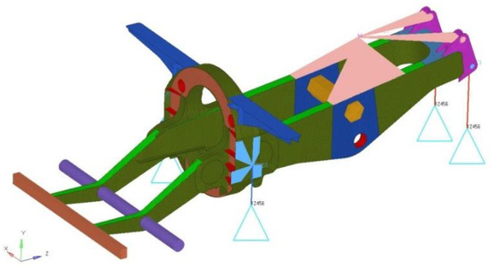
Figure 1.
Finite element model of frame.
Before estimating stiffness of the frame at intervals, the finite element model was testified. The stress due to dynamic loading in five measurement points at full load at the speed of 30 km/h on the mine road was measured, Figure 2. The strain gauge rosette was cemented in the selected zones of the frame, Figure 3 [20]. Both the results from the simulation and the road test are listed in Table 3 [20]. For point 4, the high relative error was caused by neglecting the loads at this region, because these masses from cooling system and cab were supposed to have little effect on bearing state. This high stress level could be produced by geometric mutation. The relative error of remaining measurement points all stayed within 10%, which showed that the simulated results agreed well with tested ones.
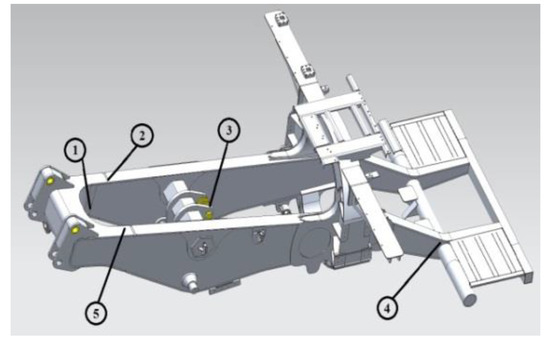
Figure 2.
Diagram of the five measurement points.
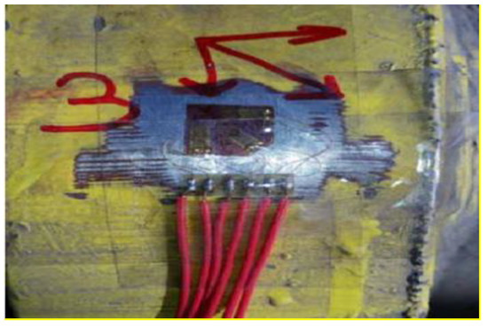
Figure 3.
The strain gauge rosette on the component.
Table 3.
Comparison of simulated results and experimental data.
The bending stiffness of frame at interval could be estimated as follows:
where expresses the interval concentrated bending load applied to the center of gravity of the goods, is wheelbase of this truck at interval, and is maximum deformation of frame in force center at interval [19]. Five finite element models and concentrated loading of frame on bending from the component project were determined. The degrees of freedom at suspensions were constrained. Then, the deformation of the frame under bending could be calculated, as listed in Table 4.
Table 4.
Initial interval values under bending.
According to Equation (7) and blind number algorithms, the total 125 probable values of bending stiffness and corresponding credibility values were obtained, and some of them are presented in Table 5. Then, the interval bending stiffness of the frame was defined by N·m2.
Table 5.
Probable values of bending stiffness and credibility.
The torsional stiffness of frame at interval could be evaluated by:
where represents concentrated torsional loading applied to the front suspension at interval, is wheelbase of this truck taking interval, is wheel-track of the truck connected with interval, and is deflection of the frame due to torsion at interval.
The other torsional condition was simulated applying to a pair of opposite loading at left and right front suspension with full constraints at rear suspension. Similarly, the torsional stiffness of frame at interval was defined by N·m2/rad.
3. Evaluation of Stress and Stiffness by Means of Latin Hypercube Sampling Method
3.1. Estimation of Stress Distribution under Three Loading Conditions
The stress state component of the frame was mainly caused by bending in horizontal plane and torsion. The stress value due to dynamic loading was evaluated using the dynamic loading coefficient [21]:
where and represent stiffness of front and rear spring systems, respectively. is self-weight, is road coefficient, is experience coefficient, is speed of truck.
This evaluation could be implemented by finite element analysis under different material parameters and dynamic coefficient. For the bending condition in horizontal plane, the weight of the full load was applied, Figure 1, and the maximum dynamic loading coefficient was calculated of 2.5 [21,22]. In order to cover all possibilities of variables, the Latin Hypercube sampling method was used. Thanks to this theory the 40 sample data were obtained. Some of them are listed in Table 6. The variables x1, x2, x3, x4 represented for the thicknesses of top longitudinal beam, stiffener, lateral longitudinal beam and hanging ear in the frame, respectively. x5, x6, n and S were deeded as Young’s modulus, Poisson’s ratio, dynamic loading coefficient and corresponding maximum equivalent stress. One of corresponding values is shown in Figure 4. The maximum equivalent stress is located at the bottom of lateral longitudinal beam around rear suspension. Then, according to the simulated maximum equivalent stress, the interval stress due to dynamic loading was calculated to be MPa. Then, these values were compared with the ultimate tensile strength at interval, Figure 5.
Table 6.
Sample data and corresponding responses.
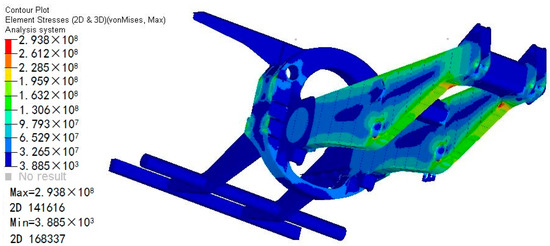
Figure 4.
Contour of vonMises stress under bending due to horizontal loading (unit: MPa).
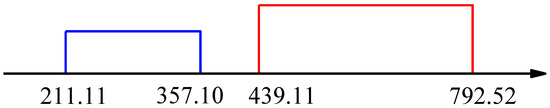
Figure 5.
Comparison of stress due to dynamic bending loading and the ultimate tensile strength at interval (unit: MPa).
The second significant condition was formulated in the following manner: an unexpected braking (fracturing) of the truck at full load. The frame is taken with a huge inertial force. Based on the distance to the fracture and time at the speed of 30 km/h for this electric wheel dump truck, the braking deceleration was calculated to be 3.816 m/s2 [21,22,23]. In this condition, the dynamic loading coefficient was equal to 1.5 [21,22,23]. The constraint was the same as the horizontal bending case. The maximum equivalent stress appeared at the same position as the bending one. Then, the stress caused by dynamic loading at interval was defined as follows , MPa, Figure 6. It was clearly seen that there was overlap between the stress and ultimate tensile strength. Therefore, the optimization design was needed.
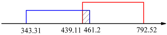
Figure 6.
Comparison of stress due to dynamic loading at breaking and ultimate tensile strength at the interval (unit: MPa).
When the truck passed pit pavement, the frame was under torsional loading. In this case, a pair of forces in opposite direction with 3.2 × 10⁶ N was applied to the left and the right front suspension [21,24]. The dynamic loading coefficient was the same as in the braking case, while only the translational degrees of freedom in vertical and longitudinal directions at rear suspensions were limited. Then, the stress due to dynamic torsion at interval was defined as , MPa, Figure 7.
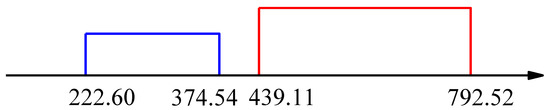
Figure 7.
Comparison of stress due to dynamic torsion and ultimate tensile strength at the interval (unit: MPa).
3.2. Estimation of Stiffness under Two Conditions at Interval
A deformation of the frame was the second aim of the analysis. It was reached basing on the frame stiffness. In order to estimate the component resistance on bending deformation, the weight of goods and carriage was applied as a kind of concentrated force in the frame, Figure 1. The translational degrees of freedom in vertical and lateral directions at front suspensions and the all translational degrees of freedom at rear suspensions were limited. Some of the 40 samples data are listed in Table 7. Fc and D are the applied force and the maximum deformation after loading, respectively. The contour of displacement in vertical direction for one sampling data is displayed in Figure 8. According to the simulated results of this bending condition and Equation (8), the bending stiffness of frame was of N·m2, Figure 9. They were exceeding the limit value and therefore the frame should be redesigned.
Table 7.
Sample data and the corresponding responses.
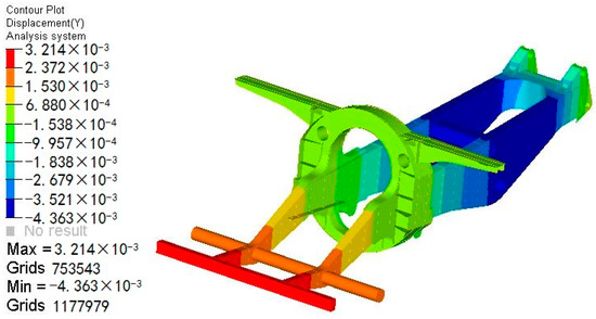
Figure 8.
Contour of displacement in vertical direction under bending (unit: m).
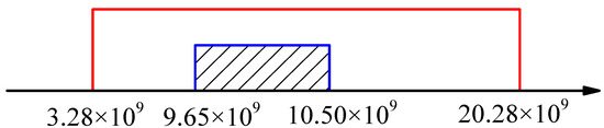
Figure 9.
Comparison of bending stiffness and its ultimate value at interval (unit: N·m2).
Similarly, the torsional stiffness assessment of frame was conducted as the approach mentioned above. The 40 sample data and their responses were obtained by finite element analysis. The contour of displacement in vertical direction for one sampling data is displayed in Figure 10. The working torsional stiffness of frame was calculated as follows: N·m2/rad, and compared with the ultimate torsional stiffness in an intersection number of axis, Figure 11. They were intersected, and thus some improvement of frame is needed.
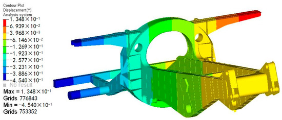
Figure 10.
Contour of displacement in vertical direction under torsion (unit: m).
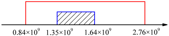
Figure 11.
Comparison of torsional stiffness and ultimate torsional stiffness at interval (unit: N·m2/rad).
4. Multi-Objectives Optimization of the Frame Based on Interval Analysis Method
An analysis of strength and stiffness of the frame under exploitation indicated that the mechanical responses under several conditions could be better. Taking uncertain factors related to manufacturing and working stages, the uncertain multi-objectives optimization design was conducted.
4.1. Interval Multi-Objectives Optimization Method
The uncertain parameters could be characterized as interval value, and the interval multi-objectives optimization function could be described as follows [25]:
where is objective function, represents constraint function. describes n-dimensional design variable within the range of , and is q-dimensional uncertain variable within the range of . and were used to mark upper and lower bound of the interval parameter, respectively. In order to ensure optimization efficiency and convergence, the uncertain objective could be transformed to the certain one and expressed by [25]:
where is the midpoint value of objective function, is the radius value of objective function. Optimizing the midpoint value could improve mean value of objective function, and optimizing the radius value could reduce the sensitivity on the uncertainties and enhance the stability and robustness for the objective function. The solution of multi-objectives optimization function could be transformed to search for the optimal result in the single-objective optimization problem, which was evaluated by [25]:
where is weight coefficient. Its range was within . In this paper, it was taken as 0.5 [25]. In this paper, the interval analysis method was utilized to optimize the frame structure for improving mechanical performances. The optimization process is shown in Figure 12.
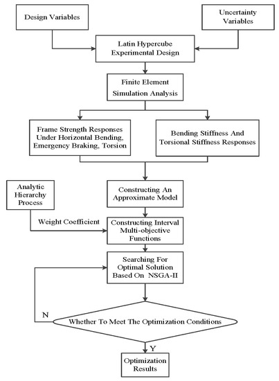
Figure 12.
Interval multi-objective optimization process.
4.2. Determination of Optimization Function and Parameters
According to the estimated results mentioned above, the strength under braking and the stiffness related to bending and torsion need to be improved. In order to avoid the conflict between optimized mechanical properties, all of them were considered as optimization objectives. In full consideration of uncertain factors during manufacturing and design stage, the thicknesses of top longitudinal beam, stiffener, lateral longitudinal beam and hanging ear in the frame were considered as design variables, and Young’s modulus and Poisson’s ratio were taken as uncertain variables [26,27]. Moreover, the constraint of design and uncertain variables was within the range of , while the range of variation for the optimization objective was ascertained from the interval allowable values.
The relationship between design variables and optimization objectives could be acquired through the response surface method. The 30 sample data for the four design variables and the six sample data for the uncertain variables were obtained by the Latin Hypercube sampling method. Some of them and their corresponding responses are listed in Table 8. The y1, y2, y3, y4 and y5 represent the stress under dynamic bending, related to dynamic braking, connected with dynamic torsion, bending stiffness and torsional stiffness, respectively.
Table 8.
Sample data and corresponding responses for constructing approximate model.
Then, according to the simulated results, the response surface model of optimization objective function was fitted by quadratic polynomial equation. Due to limited space, only model of strength in braking case was shown here:
The Pareto diagram analyzed from Equation (14) is shown in Figure 13. The design variable x3 and x1 had the most effect on optimization objective y2, and their influence ratios came to be –49.2% and –31.9%, respectively, which implied that they had negative correlation. The source item x1 – x2 had the most positive influence ratio. The main effect on optimization objective y2 is displayed in Figure 14, which shows that the variation of design variable x3 and x1 have the most influence on optimization objective y2. Then, the three-dimensional response surface between some of the design variables and optimization objective y1 is presented in Figure 15 and Figure 16. It is clearly seen that there is an approximately linear relationship between certain stress due to dynamic loading y1 and design variable x1 and x3, while there was a non-linear relationship between the stress y1 and design variables x2 and x4. Moreover, in order to testify the established response of the surface model, the other 10 sample data and their corresponding simulated results were selected to compare with the predicted ones obtained from the model. One of comparison results are shown in Figure 17 and Figure 18. Most of the points were around the equal line, which meant that the estimated results from the approximate response surface agreed well with the simulated results.
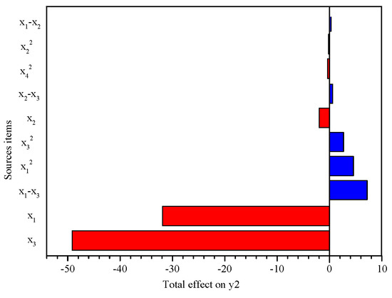
Figure 13.
Pareto diagram on y2.
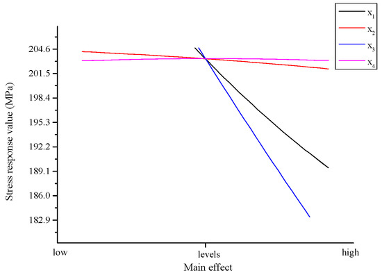
Figure 14.
Main effect on y2.
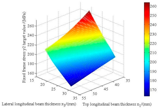
Figure 15.
Three-dimensional response model with x1 and x3.
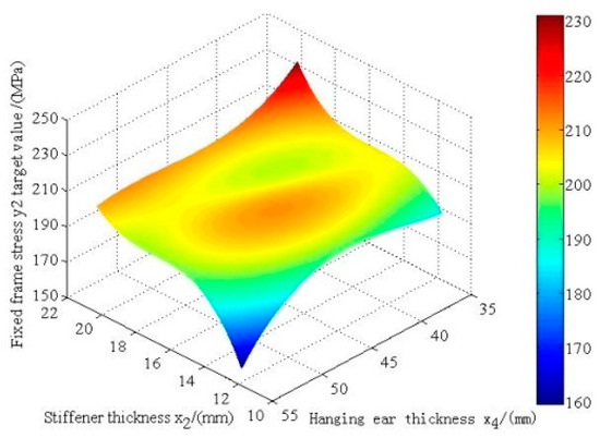
Figure 16.
Three-dimensional response model with x2 and x4.
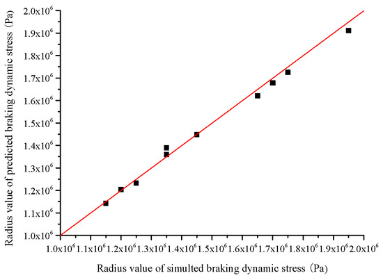
Figure 17.
Radius results between prediction and simulation.
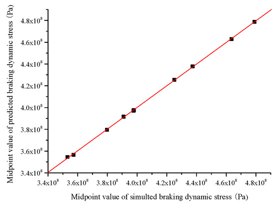
Figure 18.
Midpoint results between prediction and simulation.
4.3. Optimized Results
There were five optimization objectives for this frame, and thus the non-dominated sorting genetic algorithm was utilized to search for the optimal solution in the all sample space [28,29]. Before starting optimization design, the weight coefficient of every optimization objective had to ascertain firstly. The analytic hierarchy process method was used to calculate the coefficient. Its judgment matrix could be estimated by [30]:
where is the ratio of importance between two optimization objectives.
According to the analyzed results mentioned above and actual engineering problem, the matrix could be assigned by:
The matrix was processed to be normalized vector:
Therefore, , , , and were successively weight coefficient of five optimization objective. Then, the optimization design was implemented by software ISIGHT(Engineous, Los Angeles, CA, USA), based on the non-dominated sorting genetic algorithm. The number of populations was 200, and the number of iterations was equal to 1000. After calculating for 51 minutes, the final optimized results are listed in Table 9. Furthermore, the optimized objective values were also compared with the initial ones, Table 10. According to the optimized results, the thickness of four design variables increased, and the top longitudinal beam had the largest increase in thickness. Then, the optimization with respect to the stress related to dynamic horizontal bending, unexpected braking (fracturing) and torsion were decreased by 19.18%, 17.25% and 9.06%, respectively. The bending and torsional stiffness were improved by 21.53% and 15.88%. Obviously, the mechanical responses of this frame were enhanced with a slight increase in weight, which achieved the goal of optimization.
Table 9.
Comparison of the initial and optimized design variables.
Table 10.
Comparison of the initial and optimized certain objective values.
5. Conclusions
Based on the experimental data and finite element analysis results, the ultimate strength and stiffness of electric wheel dump truck frame at interval can be obtained through blind number theory. The stresses under dynamic horizontal bending, unexpected braking (fracturing) and torsion as well as the stiffness under bending and torsion were estimated. The thickness of main bearing beams in frame was considered as a design variable, and the material properties were regarded as uncertain variables caused by manufacturing process. Based on the response surface method, the interval multi-objectives optimization function was obtained. Finally, the non-dominated sorting genetic algorithm was used to search for the optimal solution. The specific conclusions are listed as follows:
- Based on the blind number theory, the ultimate strength of electric wheel dump truck welded frame at interval was MPa. The bending and torsional stiffness were N·m2 and N·m2/rad. Using Latin Hypercube method to acquire sample data, the stresses due to dynamic horizontal bending under horizontal bending, braking and torsional conditions were MPa, MPa and MPa, The stiffness under bending and torsion was N·m2 and N·m2/rad.
- In full consideration of the uncertain factors caused by the manufacturing process, Young’s modulus and Poisson’s ratio were considered as uncertain variables. The thickness of four main bearing beams was regarded as a design variable. Based on the non-dominated sorting genetic algorithm, the stresses due to dynamic horizontal bending in horizontal bending, unexpected braking (fracturing) and torsion were decreased by 19.18%, 17.25% and 9.06%, respectively. The bending and torsional stiffness were improved by 21.53% and 15.88%. In the meantime, all design variables were increased by approximately 15%.
Author Contributions
Conceptualization, C.M. and J.L. (Jinhua Liu); Methodology, C.M.; Software, W.L.; Validation, W.L., X.X. and J.L. (Jidong Liu); Formal analysis, C.M.; Investigation, C.M.; Resources, R.M.; Data Curation, X.X.; Writing—Original Draft Preparation, C.M.; Writing—Review & Editing, Q.Y.; Visualization, X.X.; Supervision, Q.Y.; Project Administration, C.M.; Funding Acquisition, C.M. and W.L.
Funding
This research was funded by Excellent Youth Project of Hunan Education Department (Grant No.: 18B301) and Postgraduate Research Innovation Project of Hunan Education Department (Grant No.: CX20190846) and National Natural Science Foundation of China (Grant No.: 51975192).
Acknowledgments
The authors gratefully thank for the support of Excellent Youth Project of Hunan Education Department (Grant No.: 18B301) and Postgraduate Research Innovation Project of Hunan Education Department (Grant No.: CX20190846) and National Natural Science Foundation of China (Grant No.: 51975192).
Conflicts of Interest
The authors declare no conflict of interest. The funders had no role in the design of the study; in the collection, analyses, or interpretation of data; in the writing of the manuscript, and in the decision to publish the results.
References
- Mi, C.J.; Gu, Z.Q.; Yang, Q.Q.; Nie, D.Z. Frame fatigue life assessment of a mining dump truck based on finite element method and multibody dynamics analysis. Eng. Fail. Anal. 2012, 23, 18–26. [Google Scholar] [CrossRef]
- Mi, C.J.; Li, W.T.; Wu, W.G.; Xiao, X.W. Fuzzy fatigue reliability analysis and optimization of A-type frame of electric wheel dump truck based on response surface method. Mechanika 2019, 25, 44–51. [Google Scholar] [CrossRef]
- Kim, J.; Chi, S.; Seo, J. Interaction analysis for vision-based activity identification of earthmoving excavators and dump trucks. Appl. Mech. Mater. 2018, 87, 297–308. [Google Scholar] [CrossRef]
- Mi, C.J.; Gui, Z.Q.; Zhang, Y.; Liu, S.C.; Zhang, S.; Nie, D.Z. Frame weight and anti-fatigue co-optimization of a mining dump truck based on Kriging approximation model. Eng. Fail. Anal. 2016, 66, 99–109. [Google Scholar] [CrossRef]
- Ma, X.F.; Li, T.J. Dynamic analysis of uncertain structures using an interval-wave approach. Int. J. Appl. Mech. 2018, 10, 1850021. [Google Scholar] [CrossRef]
- Tian, S.; Chen, J.H.; Dong, L.J. Rock strength interval analysis using theory of testing blind data and interval estimation. J. Cent. South Univ. 2017, 24, 168–177. [Google Scholar] [CrossRef]
- Dong, L.J.; Li, X.B. Interval parameters and credibility of representative values of tensile and compression strength tests on rock. Chin. J. Geotech. Eng. 2010, 32, 1969–1974. [Google Scholar]
- Zhang, J.; Yu, S.J. Risk analysis on groundwater resources carrying capacity based on blind number theory. Wuhan Univ. J. Nat. Sci. 2007, 12, 669–676. [Google Scholar] [CrossRef]
- Yan, H.; Zou, Z.H. Water quality evaluation based on entropy coefficient and blind number theory measure model. J. Netw. 2014, 9, 1868–1874. [Google Scholar] [CrossRef]
- Guo, P.Y.; Shi, B.Q.; Xiao, C.Y.; Yan, Y.Y.; Li, H.P. Computing-algorithm for time-dependent reliability of mechanical structure based on blind number. Trans. Chin. Soc. Agric. Mach. 2010, 198, 198–213. [Google Scholar]
- Wang, C.F.; Li, D.H.; Li, Z.; Jiang, X.Z. Optimization of controllers for gas turbine based on probabilistic robustness. J. Eng. Gas Turbines Power 2009, 131, 054502. [Google Scholar] [CrossRef]
- Zhao, Y.; Guo, Y.; Xie, K.G. Research on probability distribution characteristics of bulk power system reliability considering parameter uncertainty. Dianwang Jishu/Power Syst. Technol. 2013, 37, 2165–2172. [Google Scholar]
- Haghighi, A.; Asl, A.Z. Uncertainty analysis of water supply networks using the fuzzy set theory and NSGA-II. Eng. Appl. Artif. Intell. 2014, 32, 270–282. [Google Scholar] [CrossRef]
- Lü, H.; Shangguan, W.B.; Yu, D.J. Uncertainty quantification of squeal instability under two fuzzy-interval cases. Fuzzy Sets Syst. 2017, 328, 70–82. [Google Scholar] [CrossRef]
- Cheng, J.; Duan, G.F.; Liu, Z.Y.; Li, X.G.; Feng, Y.X.; Chen, X.H. Interval multiobjective optimization of structures based on radial basis function, interval analysis, and NSGA-II. J. Zhejiang Univ. Sci. A 2014, 15, 774–788. [Google Scholar] [CrossRef]
- Dong, J.H.; Gu, C.S.; Hao, Y.D.; Ma, F.W. Uncertainty analysis of high-frequency noise in battery electric vehicle based on interval model. SAE Pap. 2019, 3. [Google Scholar] [CrossRef]
- Fang, P.Y.; Chang, X.L.; Hu, K.; Lai, J.W.; Long, B. Reliability optimization design for turbine disk strength based on interval uncertainty. J. Propuls. Technol. 2013, 34, 962–967. [Google Scholar]
- Li, W.T.; Ni, Z.S.; Mi, C.J.; Xiao, X.W.; Liu, J.H. Interval fatigue strength analysis and optimization of A-type frame of electric wheel dump truck based on blind data theory. J. Hunan Univ. Technol. 2019. under review. [Google Scholar]
- Liu, K.D.; Wu, H.Q.; Pang, Y.J.; Wang, T.Y. The concept operations and properties of blind number. Oper. Res. Manag. Sci. 1998, 3, 16–19. [Google Scholar]
- Zhou, Y.X. Large-Tonnage Electric Wheel Dump Truck and Vibration Stress Testing and Analysis. Master’s Thesis, Hunan University of Science and Technology, Xiangtan, China, 2015; pp. 20–41. [Google Scholar]
- Yang, Q.Q.; Gu, Z.Q.; Mi, C.J.; Tao, J.; Liang, X.B.; Peng, G.P. An analysis on the fatigue life of frame in SF33900 mining dump truck. Automot. Eng. 2012, 11, 1015–1019. [Google Scholar]
- Li, Y.J. Finite element analysis of static-dynamic stress of heavy truck. Automot. Eng. 2012, 11, 35–43. [Google Scholar]
- Luo, C.L.; Zhong, X.J.; Wu, W.C. Research of blended braking characteristics of super-big electric wheels of mining dump truck. J. Guangxi Univ. (Nat. Sci. Ed.) 2012, 37, 252–258. [Google Scholar]
- Mi, C.J. Research on Frame Fatigue Reliability of Mining Dump Truck Based on the Strain Energy Method. Ph.D. Thesis, Hunan University, Changsha, China, 2014; pp. 31–76. [Google Scholar]
- Zhang, S. The Characteristics Analysis and Optimization of Heavy Duty Mining Dump Truck Vibration Reduction System Based on Interval Method. Ph.D. Thesis, Hunan University, Changsha, China, 2019; pp. 100–125. [Google Scholar]
- Li, X.L.; Jiang, C.; Han, X. An uncertainty multi-objective optimization based on interval analysis and its application. China Mech. Eng. 2011, 22, 1100–1106. [Google Scholar]
- Zhang, F.; He, X.D.; Nan, H.; Yao, H.J. Fatigue life generalized reliability analysis of the missile suspension structure considering gradual change destruction. J. Solid Rocket Technol. 2013, 5, 672–676. [Google Scholar]
- Srinivas, N.; Deb, K. Multi-objective function optimization using non-dominated sorting genetic algorithm. Evol. Comput. 1995, 2, 221–248. [Google Scholar] [CrossRef]
- Deb, K.; Agrawal, S.; Pratap, A.; Meyarivan, T. A fast and elitist multi-objective genetic algorithm: NSGA-II. IEEE Trans. Evol. Comput. 2002, 6, 182–197. [Google Scholar] [CrossRef]
- Zang, X.L.; Gui, Z.Q.; Mi, C.J.; Wu, W.G.; Jiang, J.X.; Wang, Y.T. Static/dynamic multi-objective topology optimization of the frame structure in a mining truck. Automot. Eng. 2015, 37, 566–570, 592. [Google Scholar]
© 2019 by the authors. Licensee MDPI, Basel, Switzerland. This article is an open access article distributed under the terms and conditions of the Creative Commons Attribution (CC BY) license (http://creativecommons.org/licenses/by/4.0/).