Pick and Place Operations in Logistics Using a Mobile Manipulator Controlled with Deep Reinforcement Learning

Abstract

Programming robots to perform complex tasks is a very expensive job. Traditional path planning and control are able to generate point to point collision free trajectories, but when the tasks to be performed are complex, traditional planning and control become complex tasks. This study focused on robotic operations in logistics, specifically, on picking objects in unstructured areas using a mobile manipulator configuration. The mobile manipulator has to be able to place its base in a correct place so the arm is able to plan a trajectory up to an object in a table. A deep reinforcement learning (DRL) approach was selected to solve this type of complex control tasks. Using the arm planner’s feedback, a controller for the robot base is learned, which guides the platform to such a place where the arm is able to plan a trajectory up to the object. In addition the performance of two DRL algorithms ((Deep Deterministic Policy Gradient (DDPG)) and (Proximal Policy Optimisation (PPO)) is compared within the context of a concrete robotic task.

1. Introduction

Logistics applications demand the development of flexible, safe and dependable robotic solutions for part-handling including efficient pick-and-place solutions.

Pick and place are basic operations in most robotic applications, whether in industrial setups (e.g., machine tending, assembling or bin picking) or in service robotics domains (e.g., agriculture or home). In some structured scenarios, picking and placing is a mature process. However, that is not the case when it comes to manipulating parts with high variability or in less structured environments. In this case, picking systems only exist at laboratory level, and have not reached the market due to factors such as lack of efficiency, robustness and flexibility of currently available manipulation and perception technologies. In fact, the manipulation of goods is still a potential bottleneck to achieve efficiency in the industry and the logistic market.

At the same time, the market demands more flexible systems that allow for a reduction of costs in the supply chain, increasing the competitiveness for manufacturers and bringing a cost reduction for consumers. The introduction of robotic solutions for picking in unstructured environments requires the development of flexible robotic configurations, robust environment perception, methods for trajectory planning, flexible grasping strategies and human–robot collaboration.

This study focused specifically on the development of adaptive trajectory planning strategies for pick and place operations using mobile manipulators. A mobile manipulator is a mobile platform carrying one or more manipulators. The typical configuration of mobile manipulators in industry is an anthropomorphic manipulator mounted on a mobile platform complemented with sensors (laser, vision, and ultrasonic) and tools to perform operations. The mobility of the base extends the work-space of the manipulator, which increases the operational capacity.

Currently, mobile manipulators implementation in industry is limited. One of the main challenges is to establish coordinated movements between the base and the arm in a unstructured environment depending on the application.

Although navigation and manipulation are fields where much work has been done, mobile manipulation is a less known area because it suffers from the difficulties and uncertainties of both previously mentioned fields. We propose to solve the path planning problem using a reinforcement learning (RL) strategy. The aim is to avoid explicit programming of hard-to-engineer behaviours, or at least to reduce it, taking into account the difficulty of foreseeing situations in unstructured environments. RL-based algorithms have been successfully applied to robotic applications [1] and enable learning complex behaviours only driven by a reward signal.

Specifically, this study focused on learning to navigate to such a place that the mobile manipulator’s arm is able to pick an object from a table. Due to the limited scope of the arm, not all positions near the table are feasible to pick the object and to calculate those positions analytically is not trivial. The goal of our work was to evaluate the performance of deep reinforcement learning (DRL) [2] to acquire complex control policies such as mobile manipulator positioning by learning only through the interaction with the environment. Specifically, we compared the performance of two model-free DRL algorithms, namely Deep Deterministic Policy Gradient (DDPG) and Proximal Policy Optimisation (PPO) algorithms, in two simulation tests.

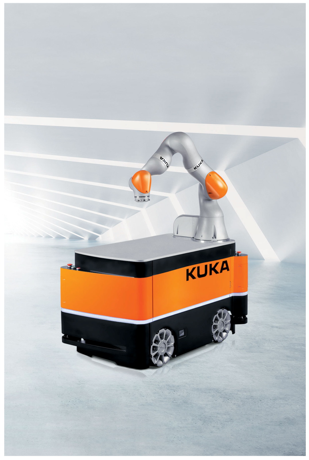
The simulated robot we used is the mobile manipulator miiwa, depicted in Figure 1, which has been used in industrial mobile manipulation tasks (e.g., [3]).

2. Literature Review

There are different approaches to establishing coordinated movements between the base and the arm depending on the application. Nassal et al. [4] specified three types of cooperation, which differ in the degree of cooperation, the associated complexity and the potential for manipulation capabilities: (1) Loose cooperation is when the mobile base and the manipulator are considered two separate systems, and the base serves as transport. There are several very well-known methods for navigation and trajectory planning [5]. (2) Full cooperation is when the two systems are seen as one (with nine degrees of freedom), and both the base and the arm move simultaneously to position the tool center. There are various approaches to solve the path planning problem [6,7], however, in these cases, the computational cost is very high. (3) Transparent cooperation is the combination of the previous two: the manipulator control compensates for the base and the base moves accordingly to maximise a cost function related to the positioning of the manipulator to perform the task. In [4], an approach to this type of control is proposed.

In general, current robotic solutions follow the loose cooperation approach. The coordination of the two subsystems for mobile manipulation depends on the task that needs to be solved. Berntorp et al. [8] addressed the issue of pick and place where the robotic system must take a can of a known position and place it in another combining the movement of the arm and the base. In [9], the problem of opening doors is considered where the movement of the arm and base are coupled by sensing the forces generated between the arm and the door, and coordinating the forward movement of the base.

One of the principal goals of artificial intelligence (AI) is to enable agents to learn from their experience to become fully autonomous. This experience is obtained by interacting with the environment. Thus, the agent should continue improving its behaviour through trial and error until it behaves optimally. Deep learning enables reinforcement learning to face decision-making problems that were previously infeasible. The union of both of them, namely DRL, makes it possible to learn complex policies guided by a reward signal and has been applied to learn multiple complex decision making tasks in a wide variety of areas. For instance, in [10], the authors learn a chess player agent by self playing that is able to defeat a world champion. In [11], DRL is used to learn an intelligent dialogue generator agent. It also has been successfully applied to computer vision, for example to train a 2D object tracker agent that outperforms state-of-the-art real-time trackers [12].

The field of DRL applied to robotics is becoming more and more popular, and the number of published papers related to that topic is increasing quickly. Applications extend from manipulation [13,14,15,16] to autonomous navigation [17,18] and locomotion [19,20].

DRL has been successfully applied in some robotic path planning and control problems. For example, Gu et al. [16] used DRL to learn a low-level controller that is able to control a robotic arm to perform door opening. On the one hand, 25 variables are used to represent the environment’s state. More specifically, those variables correspond to the joint angles and their time derivatives, the goal position and the door angle together with the handle angle. On the other hand, the action is represented by the torque for each joint. Robot navigation is another area where DRL also has been applied successfully; for example, in [18], DRL is applied to learn a controller to perform mapless navigation with a mobile robot. In this work, a low dimensionality state representation is also used, specifically 10-dimensional laser range findings, the previous action and the relative target position. The action representation includes linear and angular velocities of the differential robot.

Alternatively, several methods use 2D or 3D images instead of low-dimensional state representations. In [15], for example, 2D images are used with the goal of learning grasping actions. The authors tried to map images directly with low-level control actions and, in addition, the developed system is able to generalise and pick objects that the model has not been trained with. Moreover, other applications (e.g., [21]) use 3D depth images as state representation, but instead of learning directly from pixels, they encode the images to a lower dimensional space before training the model. This encoding enables to accelerate the training process.

Although there are multiple works about learning to control either robotic arms and mobile bases, to the best of our knowledge, references about DRL applied to mobile manipulation are few. The goal of this paper is to show that it is possible to use the arm path planner’s feedback to learn a low-level controller for the base. The learned controller is able to guide the robot to a feasible pose in the environment to do the picking trial. To do that, a low-dimensional state representation is used.

In [22], the authors proposed to learn, through interaction with the environment, which place is the best to locate the base of a mobile manipulator, in such a way that the arm is able to pick an object from a table. In that way, the robot takes into account its physical conditions and also the environment’s conditions to learn which is the optimal place to perform the grasping action. In this case, they acquire experience off-line, and, after applying some classifiers, such as support vector machines, they are able to learn a model that maps the state of the robot with some feasible places in the environment to do the picking trial. Then, the trained model is used on-line.

In comparison with the previous approach, the goal of the RL-based algorithms is to learn on-line, while the agent interacts with the environment, improving its policy until it reaches to the optimal behaviour. In addition, the goal of our work is to learn a controller, which gives a low-level control signal in each state to drive the mobile robot, while, in [22], instead of learning a controller to drive the robot up to the optimal pose, they tried to find directly which is the optimal pose.

3. Methodological Approach

According to Sutton and Barto [23], a reinforcement learning solution to a control problem is defined as a finite horizon Markov Decision Process (MDP). At each discrete time-step t, the agent observes the current state of the environment $s_t\in S$, takes an action $a_t\in A\left(s_t\right)$, receives a reward $r:S\times A\to \mathbb{R}$ and observes the new state of the environment $s_{t+1}$. At each episode of T time-steps, the environment and the agent are reset to their initial poses. The goal of the agent is to find a policy, deterministic ${\pi }_{\theta }\left(s\right)$ or stochastic ${\pi }_{\theta }\left(a\right|s)$, parameterised by $\theta$ under which the expected reward is maximised.

Traditional reinforcement learning algorithms are able to deal with discrete state and action spaces but, in robotic tasks, where both state and action spaces are continuous, discretising those spaces does not work well. Nevertheless, most state-of-the-art algorithms use deep neural networks to map observations with low-level control actions to be able to deal with continuous spaces. In our approach, a DRL algorithm is used to learn where to place the mobile manipulator to make a correct picking trial through the interaction with the environment. Those DRL algorithms need a huge amount of experience to be able to learn complex robotic behaviours and, thus, it is infeasible to train them acquiring experience in real world. In addition, the actions taken by the robot in the initial learning iterations are nearly random and both the robot and the environment might end up damaged as a result. Therefore, DRL algorithms are usually trained in simulation. Learning in simulation enables a faster experience acquisition and avoids material costs. Our study used a simulation-based approach, and we based it on open source robotic tools such as Gazebo simulator, Robot Operating System (ROS) middleware [24], OpenAI Baselines DRL library [25] and Gym/Gym-gazebo toolboxes [26,27].

DRL algorithms follow value-based, policy search or actor–critic architectures [28]. Value based-algorithms estimate the expected reward of an state or state–action pair and are able to deal with discrete action spaces, typically using greedy policies. To be able to deal with continuous action spaces, policy search methods use a parameterised policy and do not need a value function. Usually, those methods have the difficulty of not easily being able to evaluate the policy and they have high variance. Actor–critic architecture is the most used one in the state-of-the-art algorithms and combines the benefits of the two previous algorithm types. On the one hand, actor–critic-based methods use a parameterised policy (actor), and, on the other hand, use a value or action–value function that evaluates the quality of the policy (critic).

The proposed approach follows the actor–critic architecture. On the one hand, a parameterised policy ${\pi }_{\theta }$ is used to be able to deal with both continuous state and action spaces in stochastic environments, encoded by the parameter vector $\theta$. On the other hand, a parameterised value function is used to estimate the expected reward at each state or state–action pair, where w is the parameter vector that encodes the critic. The state value function $V_w\left(s\right)$ estimates the expected average reward of all actions in the state s. The action–value function $Q_w(s,a)$, instead, estimates the expected reward of executing action a in state s. Then, the critic’s information is used to update both actor and critic. In DRL algorithms, both actor and critic are parameterised by deep neural networks, and the goal is to optimise those parameters to get the agent’s optimal behaviour.

In addition, DRL algorithms are divided into two groups, on-policy and off-policy, depending on how they are able to acquire experience. On-policy algorithms expect that the experience used to optimise their behaviour policy is generated by the same policy. Off-policy methods, instead, can use experience generated by another policy to optimise its behaviour policy. Those methods are said to be able to better explore the environment than on-policy methods because they use a more exploratory policy to get experience. In this study, we compared an on-policy algorithm and an off-policy algorithm, to see which type of methods adjusts better to our mobile manipulation behaviour learning. Specifically, PPO and DDPG were used, being those on-policy and off-policy, respectively. The first one learns stochastic policies, which maps states with actions represented by Gaussian probability distributions. DDPG, instead, is able to deterministically map states with actions. Both algorithms follow actor–critic architecture.

3.1. Algorithms

In this section, we describe the theoretical basis of PPO and DDPG.

3.1.1. PPO

PPO [29] follows the actor–critic architecture and it is based on the trust-region policy optimisation (TRPO) [30] algorithm. This algorithm aims to learn a stochastic policy ${\pi }_{\theta }\left(a_t\right|s_t)$ that maps states with Gaussian distributions over actions. In addition, the critic is a value function $V_w\left(s_t\right)$ that outputs the mean expected reward in state $s_t$. This algorithm has the benefits of TRPO and in general of trust region based methods but it is much simpler to implement it. The intuition behind trust-region based algorithms is that, at each parameter update of the policy, the output distribution cannot diverge too much from the original distribution.

To update the actor’s parameters, a clipped surrogate objective is used. Although another loss function is also proposed, using a Kullback–Leibler (KL) divergence [31] penalty on the loss function instead of the clipped surrogate objective, the experimental results obtained are not as good as with the clipped one. Let $r_t\left(\theta \right)$ denote the probability ratio defined in Equation (1), so that $r_t\left({\theta }_{old}\right)=1$.

$$r_t\left(\theta \right)=\frac{{\pi }_{\theta }\left(a_t\right|s_t)}{{\pi }_{{\theta }_{old}}\left(a_t\right|s_t)}$$

(1)

${\theta }_{old}$ is the actor’s parameter vector before the update. The objective of TRPO is to maximise the objective function $L\left(\theta \right)$ defined in Equation (2). Here, $\mathbb{E}[\dots ]$ indicates the average over a finite batch of samples. The usage of the advantage ${\widehat{A}}_t$ in policy gradient algorithms was popularised by Schulman et al. [32] and indicates how good the performed action is with respect to the average actions performed in each state. To compute the advantages, the algorithm executes a trajectory of T actions and computes them as defined in Equation (3). Here, t denotes the time index $[0,T]$ in the trajectory of length T and $\gamma$ is the discount factor.

$$L\left(\theta \right)=\mathbb{E}\left[\frac{{\pi }_{\theta }\left(a_t\right|s_t)}{{\pi }_{{\theta }_{old}}\left(a_t\right|s_t)}{\widehat{A}}_t\right]$$

(2)

$${\widehat{A}}_t=-V_w\left(s_t\right)+r_t+\gamma r_{t+1}+\dots +{\gamma }^{T-t+1}{r}_{T-1}+{\gamma }^{T-t}{V}_w\left(s_T\right)$$

(3)

At each policy update, if the advantage has a positive value, the policy gradient is pushed in that direction because it means that the action performed is better than the average. Otherwise, the gradient is pushed in the opposite direction.

Without any constraint, the maximisation of the loss function $L\left(\theta \right)$ would lead to big changes in the policy at each training step. PPO modifies the objective function so that penalises big changes in the policy that move $r_t\left(\theta \right)$ away from 1. Maintaining $r_t\left(\theta \right)$ near to 1 ensures that, at each policy update, the new distribution does not diverge to much from the old one. The objective function is defined in Equation (4).

$$L^{CLIP}\left(\theta \right)=\mathbb{E}\left[min(r_t\left(\theta \right){\widehat{A}}_t,clip(r_t\left(\theta \right),1-ϵ,1+ϵ)){\widehat{A}}_t\right]$$

(4)

Here, $ϵ$ is a hyper-parameter that changes the clip range.

To update the value function $V_w\left(s\right)$ (the critic), the squared-error loss function is used (Equation (5)) between the current state value and a target value. The target value is defined in Equation (6).

$$J\left(w\right)={(V_w\left(s_t\right)-V_t^{targ})}^2$$

(5)

$$V_t^{targ}={\widehat{A}}_t+V_w\left(s_t\right)$$

(6)

The PPO algorithm is detailed in Algorithm 1. Although this algorithm is designed to be able to have multiple parallel actors getting experience, only one actor is being used.

Algorithm 1 Proximal Policy Optimisation (PPO).

1: for$e\in episodes$do 2:     for $a\in actors$ do 3:         Run policy ${\pi }_{{\theta }_{old}}$ in environment for T time-steps 4:         Compute advantage estimates ${\widehat{A}}_1\dots {\widehat{A}}_T$ 5:     end for 6:     Optimise actor’s loss function $L^{CLIP}$ with regard to $\theta$, with K epochs and minibatch size N $\le T·actors$ 7:     ${\theta }_{old}\leftarrow \theta$ 8: end for

3.1.2. DDPG

DDPG [33] combines elements of value function based and policy gradient based algorithms, following the actor–critic architecture. This algorithm aims to learn a deterministic policy ${\pi }_{\theta }\left(s\right)=a$ and it is derived from the deterministic policy gradient theorem [34].

Following the actor–critic architecture, DDPG uses an action–value function $Q_w(s,a)$ as critic to guide the learning process of the policy and it is based on the deep Q-network (DQN) [35]. Prior to DQN, it was believed that learning value functions with large and nonlinear function approximators was difficult. DQN is able to learn robust value functions due to two innovations: First, the network is trained off-policy getting experience samples from a replay buffer to eliminate temporal correlations. In addition, target networks are used, which are updated more slowly, and this gives consistent targets during temporal difference learning.

The critic is updated according to the gradient of the objective defined in Equation (7).

$$L\left(w\right)=\mathbb{E}\left[{(Q_w(s_t,a_t)-y_t)}^2\right]$$

(7)

where

$$y_t=r(s_t,a_t)+\gamma Q_w(s_{t+1},a_{t+1}){|}_{a_{t+1}={\pi }_{\theta }\left(s_{t+1}\right)}$$

(8)

The actor is updated following the deterministic policy gradient theorem, defined in Equation (9). The intuition is to update the policy in the direction that improves $Q_w(s,a)$ most.

$$\mathsf{\nabla }J\left(\theta \right)=\mathbb{E}\left[{\mathsf{\nabla }}_{\theta }{\pi }_{\theta }\left(s_t\right){\mathsf{\nabla }}_a{Q}_w(s_t,a_t){|}_{a={\pi }_{\theta }\left(s_t\right)}\right]$$

(9)

As mentioned before, the target value defined in Equation (8) is calculated using the target networks ${\pi }_{{\theta }^{\prime }}^{\prime }$ and $Q_{w^{\prime }}^{\prime }$, which are updated more slowly and this gives more consistent targets when learning the action–value function.

As DDPG is an off-policy algorithm, the policy used to get experience is different from the behaviour policy. Despite the behaviour policy being deterministic, typically, a stochastic policy is used to get experience, being able to better explore the environment. This exploratory policy is usually achieved adding noise to the behaviour policy. Although there are common noises such as normal noise or Ornstein–Uhlenbeck noise [36], which are added directly to the action generated by the policy, in [37], Plapperta et al. proposed adding noise to the neural network’s parameter space to improve the exploration and to reduce the training time. The DDPG algorithm is described in Algorithm 2.

Algorithm 2 Deep Deterministic Policy Gradient (DDPG).

1: Initialise the actor ${\pi }_{\theta }\left(s\right)$ and the critic $Q_w(s,a)$ networks. 2: Initialise the target networks $Q^{\prime }$ y ${\pi }^{\prime }$ with the weights ${\theta }^{\prime }\leftarrow \theta$, $w^{\prime }\leftarrow w$ 3: Initialise the replay buffer 4: for$e\in episodes$do 5:     Initialise noise generation process 6:     Get the first observation 7:     for $t\in steps$ do 8:         Select the action $a_t={\pi }_{\theta }\left(s_t\right)+N$ 9:         Execute the action $a_t$, get the reward $r_t$ and the observation $s_{t+1}$ 10:         Store the transition $<s_t,a_t,r_t,s_{t+1}>$ in replay buffer 11:         Get M experience samples $<s_i,a_i,r_i,s_{i+1}>$ from the replay buffer 12:         $y_i=r_i+\gamma Q_{w^{\prime }}^{\prime }(s_{i+1},{\pi }_{{\theta }^{\prime }}^{\prime }\left(s_{i+1}\right))$ 13:         Update the critic minimising the loss : $$L=\frac{1}{M}\sum _i{(y_i-Q_w(s_i,a_i))}^2$$ 14:         Update the policy of the actor: $${\mathsf{\nabla }}_{\theta }J\approx \frac{1}{M}\sum _i{\mathsf{\nabla }}_a{Q}_w(s,a){{|}_{s=s_i,a={\pi }_{\theta }\left(s_i\right)}{\mathsf{\nabla }}_{\theta }{\pi }_{\theta }\left(s\right)|}_{s=s_i}$$ 15:         Update target networks: $${\theta }^{\prime }\leftarrow \tau \theta +(1-\tau ){\theta }^{\prime }$$ $$w^{\prime }\leftarrow \tau w+(1-\tau )w^{\prime }$$ 16:     end for 17: end for

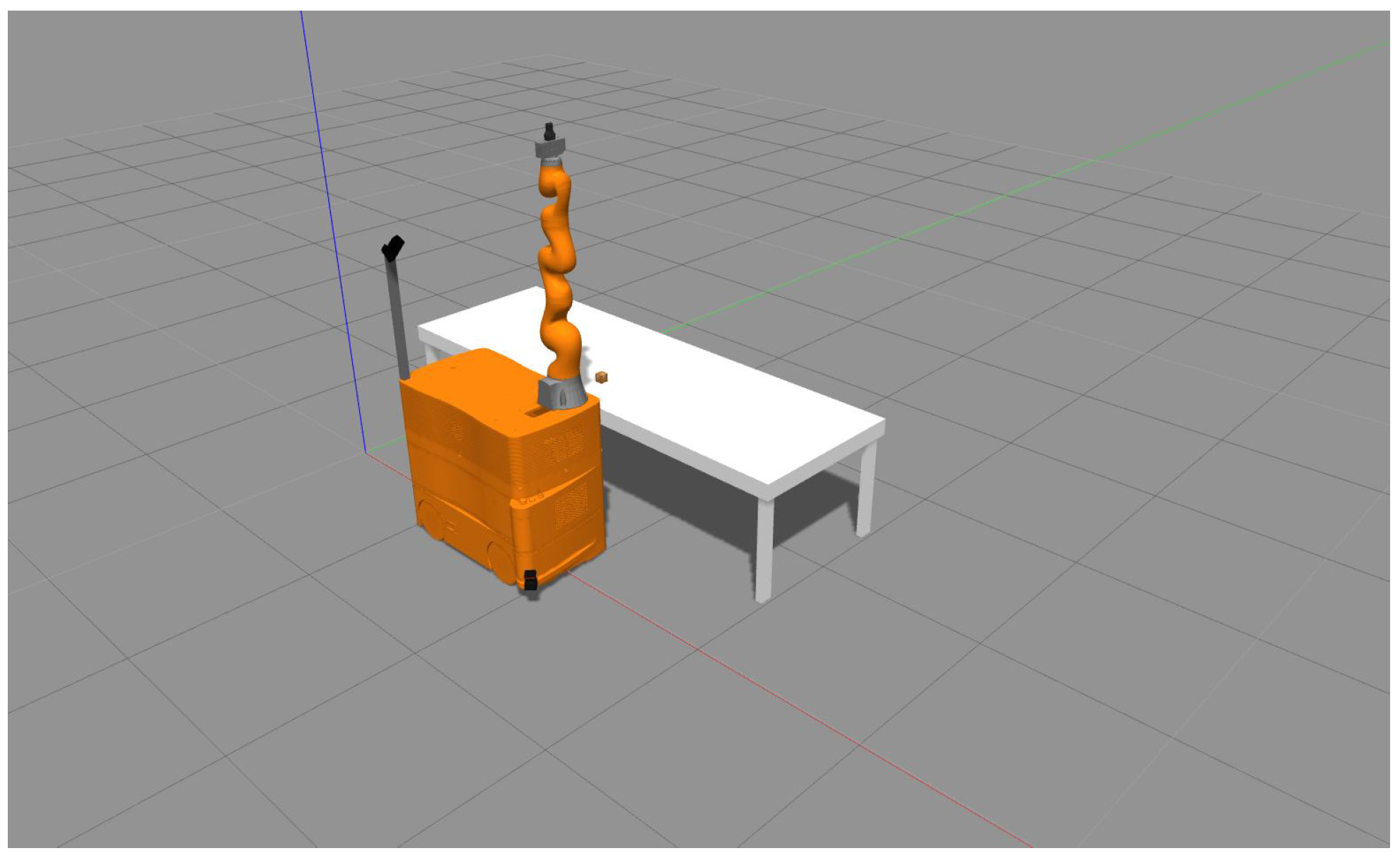
3.2. Simulated Layout

To model our world, we used the Gazebo model based simulator. The elements that are placed in this simulated world are the robot miiwa, the table and an object, which is on top of the table, as depicted in Figure 2.

The mobile manipulator miiwa is composed of a 7 DoF arm and a 3 DoF omnidirectional mobile base. To be able to control the mobile base, the gazebo planar move plugin was used.

To test if our environment was modelled correctly and to know if the algorithms could learn low-level control tasks in that environment, the learning process was divided into two simulation tests. In both, the algorithm must learn to control the mobile base with velocity commands, such that, at each discrete time-step, the algorithm gets the state of the environment and publishes a velocity command. The objective of those tests was to learn a low-level controller to drive the robot to a place where the arm can plan a trajectory up to the object on the table. To learn those controllers, the feedback of the arm’s planner was used. The summary of the tests is listed in

Table 1. Test setup summary.

Test	Robot Initial Pose	Box Initial Pose	Objective
Test 1	Variable	Variable	The arm to be able to plan a trajectory up to the box
Test 2	Variable	Constant	To plan a trajectory with an obstacle in the table

.

4. Implementation

The application was implemented in a modular way using ROS for several reasons. On the one hand, it enabled us to modularise the application and to parallelise processes. On the other hand, Gazebo is perfectly integrated with ROS and offers facilities to control the simulation using topics, services and actions.

OpenAI Gym is a toolkit to do research on DRL algorithms and to do benchmarks between DRL algorithms. This library includes some simulated environments that are used to test the quality of new algorithms and its use is widespread in the DRL community. Gym offers simple functions to interact with the environments, which are mostly modelled in the Mujoco [38] simulator. Due to the simplicity of the interface that Gym offers, it has become a standard way to interact with environments in DRL algorithms. Gym-gazebo is an extension of Gym that enables the user to create robotic environments in Gazebo and offers the same simple interface to the algorithm to be able to interact with the environment. All the environments we modelled were integrated with Gym-gazebo, which enabled us to straightforwardly use OpenAI Baselines DRL library, which is designed to work with Gym.

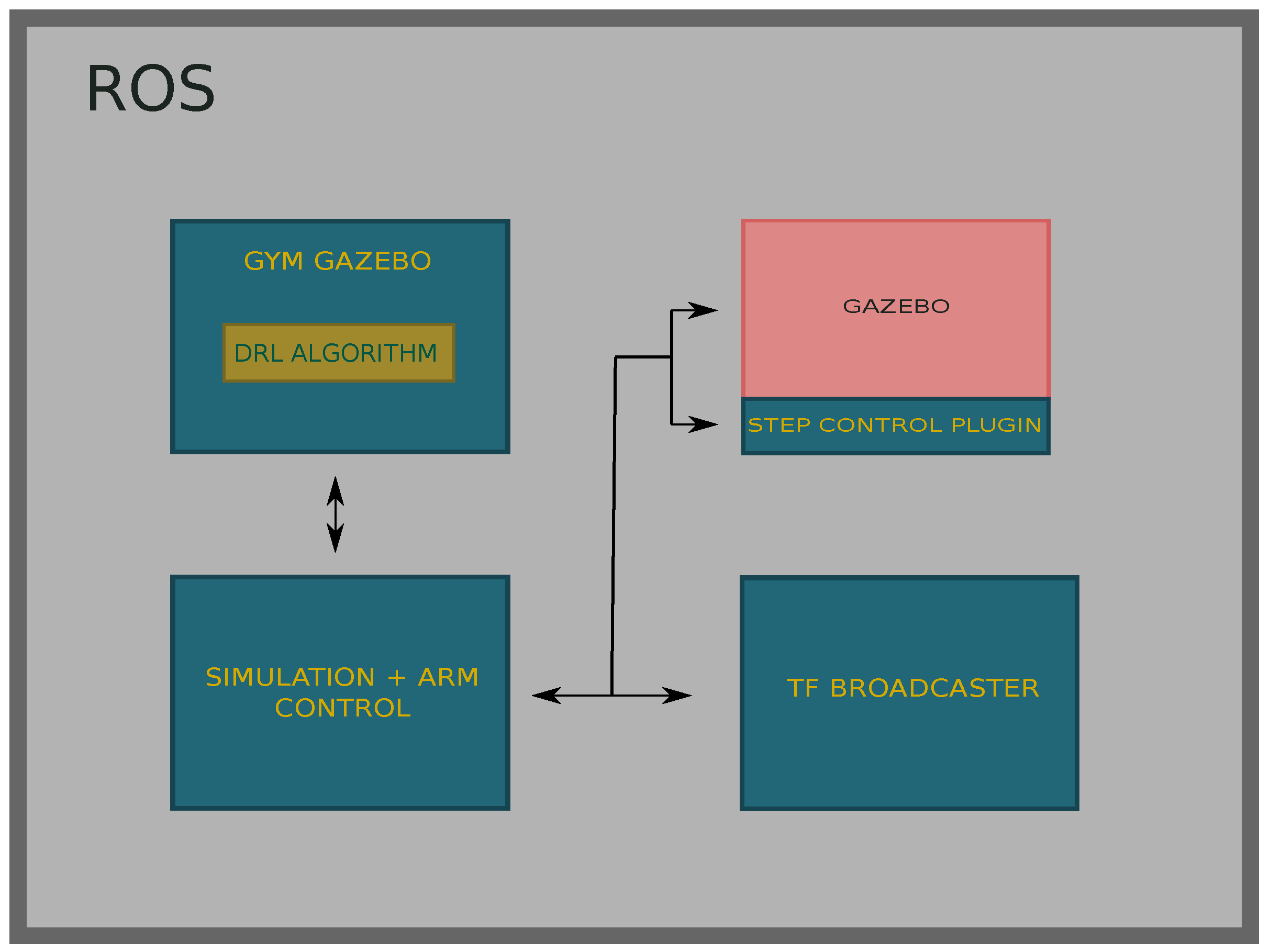
Gym-gazebo wraps the used DRL algorithms in ROS nodes and enables interaction with the environment. Nevertheless, another ROS node has been developed that is in charge with controlling all the elements of the simulation and works as bridge between the Gym-gazebo node and the simulator. To be able to control the simulation physic updates and to compute them as fast as possible, we developed a Gazebo plugin, which in turn is a ROS node. Thus, using ROS communication methods, we could control each simulated discrete time-step and we simulated those steps faster than real time. Specifically, this node takes care of all time-steps being of the same length, executing a fixed number of physic updates at each step.

The tf broadcaster node uses the tf tool that ROS offers to keep track of all the transformations between frames. We used this node to publish some transformations such as the transformation between the object and world frames. Consequently, the robot is always aware of where the object is in order to be able to navigate up to it. The implemented architecture is shown in Figure 3.

4.1. Simulation

The learning process was carried out during a fixed number of time-steps, which were divided into episodes of 512 time-steps. Gazebo’s max step size $T_m$ is an important parameter that indicates the time-step at which Gazebo computes successive states of the model. The default value is 1 ms, but, in this case, $T_m=2$ ms was used, which gave enough stability and enabled a faster simulation. Thus, each iteration of the physic engine meant 2 ms of simulated time and those iterations could be computed as quickly as possible to be able to accelerate the simulation. Besides, the real time update rate $U_r$ parameter indicates how many physic iterations will be tried in one second. The real time factor is defined in Equation (10) and indicates how much faster the simulation goes in comparison with the real time. Thus, $rtf=1$ indicates that the simulation is running on real time.

$$rtf=T_m·U_r$$

(10)

In addition, a frame-skip $N_{T_m}$ was defined to be able to get a reasonable control rate. In this application, $N_{T_m}=4$ was used so the discrete time-step size is defined in Equation (11) and doing that we achieve a control rate of 125 Hz.

$$T_s=T_m·N_{T_m}=8\mathrm{ms}$$

(11)

Thus, the length of each discrete time-step is 8 ms and those steps are computed faster than real time. Gazebo does not allow the control of the physics engine iterations, so a Gazebo plugin was developed to be able to execute the simulation for some iterations and to be able to compute those iterations as fast as possible. When the plugin was told to run a time-step, it ran $N_{T_m}$ physics iterations and the real time update rate was set to 0 to compute those iterations as quickly as possible. Doing this, the real time factor increased and enabled us to run the simulation about 5–10 times faster than in real time.

At each step, the learning algorithm generates an action, specifically a velocity command, which is sent to the mobile base. After executing it and at the end of the step, a reward signal is given evaluating the quality of the action performed by the base. The action is the same for all the experiments and is defined in Equation (12).

$$a=\left[v_x{v}_y{\omega }_z\right]$$

(12)

To be able to control the mobile base, the gazebo planar move plugin was used, which enabled the sending of velocity commands to the omnidirectional base. In addition, it published the odometry information, which was used to know where the robot is respect to a parent coordinate frame. The path planning and control of the arm was made using MoveIt! [39] and enabled us to plan collision free trajectories. Besides that, MoveIt! uses an internal planning scene where objects can be added to be taken into account when the trajectory is planned.

4.2. Network Architectures

The library of DRL algorithms used is OpenAI Baselines. This library offers high quality implementations of many state-of-the-art DRL algorithms implemented in Tensorflow [40]. Although the implementation offers complex networks such as convolutional neural networks (CNN) or recurrent neural networks (RNN), we used fully connected multi-layer perceptrons (MLP) to parameterise both policies and value functions.

4.2.1. PPO

The network architecture used in this algorithm is the one proposed by Schulman et al. [29] in the original paper. To parameterise both the policy ${\pi }_{\theta }\left(a_t\right|s_t)$ and the value function $V_w\left(s_t\right)$, a four layered MLP was used. In both actor and critic, the first layer’s size depends on the size of the state encoding, which was different in each test. The actor’s input layer is followed by two hidden layers of 64 neurons each. The output layer’s size depends on the action space’s size. In this case, the action was a vector of three elements representing the velocity command, which has to be sent to the mobile base. Specifically, the velocity command is composed of the linear velocities in x and y axes, and the angular velocity in z axis. As mentioned before, this algorithm uses a stochastic policy and, thus, each action is defined by a Gaussian distribution. Each distribution is characterised by a mean and a standard deviation. Hence, the neurons of the last hidden layer are fully connected with the mean of each action. In addition, three variables are used to store and update the standard deviation.

The activation function applied to the output of each neuron of the hidden layers is Tanh. Instead, no activation function is applied to the output of the neurons of the last layer.

Regarding the value function $V_w\left(s_t\right)$, the first three layers have the same architecture as the actor’s first three layers. The output layer, instead, is composed of a single neuron, which is fully connected with each neuron of the last hidden layer and outputs the expected average reward of a state. The activation function used in the hidden layers is Tanh as well.

4.2.2. DDPG

The network architecture used is the default implementation that the OpenAI Baselines library offers, which is very similar to the architecture proposed by Lillicrap et al. [33]. As in PPO, to parameterise both the policy ${\pi }_{\theta }\left(s_t\right)$ and the action–value function $Q(s_t,a_t)$, a four layered MLP was used. This algorithm aims to learn a deterministic policy so each state will be mapped with a concrete action. The actor’s input layer also depends on the state encoding and it is followed by two hidden layers, composed of 64 neurons each. Concerning the output layer, it is composed of three neurons, one per action, and each neuron is fully connected with each neuron of the last hidden layer.

With respect to the activation functions, the Rectified Linear Unit (ReLU) function is used in each neuron of the hidden layers. In the output layer, instead, Tanh is used to bound the actions between −1 and 1. In addition, a process called layer normalisation [41] is applied to the output of each hidden layer to simplify the learning process and to reduce the training time. DDPG is an off-policy algorithm, hence it uses a more exploratory policy to get experience. As explained in the algorithm’s description (Section 3.1.2), there are multiple types of noise but, in this application, the noise is added in the neural network’s parameter space.

The action–value function $Q_w(s,a)$ receives as input the state and the action and outputs the expected future reward of executing action $a_t$ in state $s_t$. The input layer depends on the size of the state codification. The input layer is followed by two hidden layers of 64 neurons each and actions are not included until the second hidden layer. The output layer only has one neuron and outputs the q-value. The activation function used in the critic network is ReLU for each neuron of the hidden layers. The last layer’s neurons do not have any activation function, because the action–value does not have to be bounded.

To minimise the complexity of the critic and to avoid over-fitting, a $L2$ regularisation term is added to the critic’s loss function [42]. This penalises the model for having parameters with high values.

4.3. Test Setup

Here, we describe the simulation setup in addition to the state codification and the reward function we used in each test. For both PPO and DDPG, the setup and reward functions were the same in all tests.

The robot’s work-space is limited and a new episode starts when it goes out of limits. Those limits are defined in Equation (13).

$$x_r^w=[-1.0,3.0]y_r^w=[-1.5,0.0]$$

(13)

In addition, although the robot was penalised by navigating with high speed, the environment bounds the velocities applied to the mobile base. The maximum linear velocity in x and y axes was 1 m/s and the maximum angular velocity in z axis was 1 rad/s. Thus, if the algorithm predicted velocities higher than those, the limit velocities were applied and the agent was penalised proportionally. Besides, high accelerations were also penalised proportionally, but in this case the environment did not bound them.

The learning process was divided into episodes where the robot had T time-steps to complete the task. The episode length was $T=512$ time-steps, which is about 4 s, and a discrete time-step t was terminal if:

• The robot collides with the table.
• Robot poses out of limits.
• $t=T$.

The tuning hyper-parameters used in each algorithm are described in

Table 2. Hyper-parameters.

PPO Setup Hyper-Parameters
Actor/Critic learning rate	$f\left(step\right)=step$·$3\times {10}^{-4}$
Clip-range	0.2
Discount factor $\gamma$	0.99
Batch size	512
Mini-batch size	64
Updates	${\displaystyle \frac{trainingtime\_steps}{batch\_size}}$
Training epochs per update	10
DDPG Setup Hyper-Parameters
Actor’s learning rate	$1\times {10}^{-4}$
Critic’s learning rate	$1\times {10}^{-3}$
Batch size	128
Discount factor $\gamma$	$0.99$
Critic l2 regularisation	$1\times {10}^{-2}$
Running epochs	500
Cycles per epoch	10
Rollouts per cycle	512
Updates	$epochs·cycles$
Training iterations per update	100

and were not changed across tests.

4.3.1. Test 1

Here, the objective was to learn a controller that guides the robot to a place near the table so that the arm could plan a trajectory up to the object. The robot and object initial poses were variable, which are defined in Equations (14) and (15). The robot’s initial $y_r^w$ coordinate was constant so that the robot always began at the same distance from the table. The state codification is defined in Equation (16) and it is composed of the following 10 variables:

• Robot’s position in world coordinate system: $x_r^w,x_r^w$
• Robot’s rotation on z axis in world coordinate system: $ya{w}_r^w$
• Robot’s linear velocities on x and y axes: $v_x,v_y$
• Robot’s angular velocity in z axis: ${\omega }_z$
• Object’s position in world coordinate system: $x_{obj}^w,y_{obj}^w$
• Distance between the robot and the object: $d(p_r,p_{obj})$
• Remaining time steps to end the episode: t

  $$x_r^w=[0.0,3.0]y_r^w=-1.5ya{w}_r^w=[-\pi ,\pi ]$$

  (14)

  $$x_{obj}^w=[0.5,2.5]y_{obj}^w=[0.5,0.75]z_{obj}^w=1.2$$

  (15)

  $$s=\left[x_r^w{y}_r^{w}ya{w}_r^w{v}_x{v}_y{\omega }_z{x}_{obj}^w{y}_{obj}^{w}d(p_r,p_{obj})t\right]\in {\mathbb{R}}^{10}$$

  (16)

The linear and the angular velocities included in the state were the velocities sent in the previous time-step to the robot (previous action). The reward function used is defined in Equation (17). A nonlinear function was used to give higher rewards when the robot was close to the object and high velocities and accelerations were penalised to encourage smooth driving. Here, $\Delta v$ means the velocity difference (acceleration) between current and previous action. Instead, v_high penalised each linear or angular velocity being higher than a threshold. As mentioned before, the maximum linear and angular velocities were 1 m/s and 1 rad/s, respectively. In addition, in the last time-step of the episode, an additional reward was given if the arm could plan a trajectory up to the object. The number of remaining time-steps was included in the state for robot to be aware when this last step was coming. The collision variable was equal to 1 when a collision occurred, and 0 otherwise.

$$r(s_t,a_t)=\frac{1}{d(p_r,p_{obj})}·(1-collision)-0.5·\Delta v-0.5·v\_high\left(a_t\right)+100·success$$

(17)

$$v\_high\left(a_t\right)=\sum _{i=1}^3{a}_{t_i},\mathrm{if}{a}_{t_i}>k$$

(18)

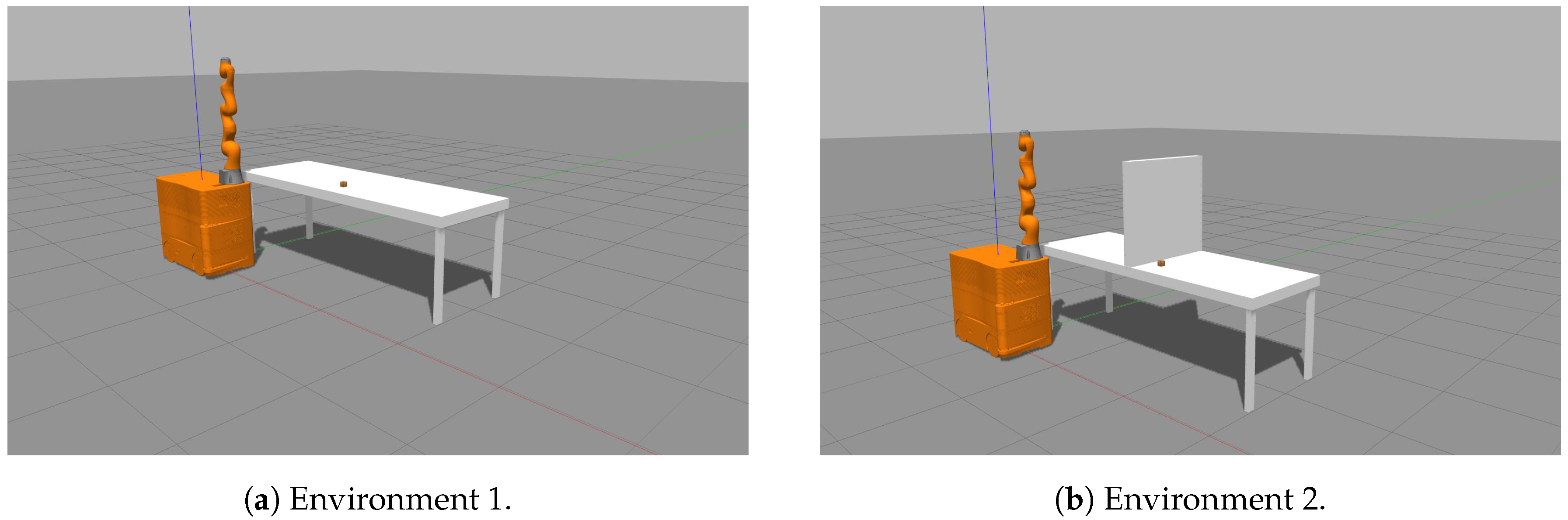
4.3.2. Test 2

In this test, as in the previous one, the robot had to navigate to a place near the table such that the arm could plan a trajectory up to the object in the table. In this case, a wall was placed near the object to see if the algorithm could discard poses that were behind the wall. The robot’s initial pose was variable (Equation (19)) and the object’s initial pose was constant (Equation (20)). As in the first test, the robot’s initial $y_r^w$ coordinate was constant so that the robot always began at the same distance from the table. The state codification defined in Equation (21) is composed of the following 8 variables:

• Robot’s position in object’s coordinate system: $x_r^{obj},x_r^{obj}$
• Robot’s rotation on z axis in object’s coordinate system: $ya{w}_r^{obj}$
• Robot’s linear velocities on x and y axes: $v_x,v_y$
• Robot’s angular velocity in z axis: ${\omega }_z$
• Distance between the robot and object’s coordinate system origin: $d(p_r,\mathbb{O})$
• Remaining time steps to end the episode: t

  $$x_r^w=[0.0,3.0]y_r^w=-1.5ya{w}_r^w=[-\pi ,\pi ]$$

  (19)

  $$x_{obj}^w=1.7y_{obj}^w=0.75z_{obj}^w=1.005$$

  (20)

  $$s=\left[x_r^{obj}{y}_r^{obj}ya{w}_r^{obj}{v}_x{v}_y{\omega }_{z}d(p_r,\mathbb{O})t\right]\in {\mathbb{R}}^8$$

  (21)

The used reward function is defined in Equation (22). In this case, the distance was computed between the robot’s position $p_r$ and object’s coordinate system origin $\mathbb{O}$.

$$r(s_t,a_t)=\frac{1}{d(p_r,\mathbb{O})}·(1-collision)-0.5·\Delta v-0.5·v\_high\left(a_t\right)+100·success$$

(22)

The environments used in the first and second tests are depicted in Figure 4a,b, respectively.

5. Results

The learning process was carried out during a fixed number of time-steps and, to be able to evaluate the performance of the algorithms, several evaluation periods of 10 episodes each were made. Specifically, 500 evaluation periods were made uniformly distributed over the learning process and the metrics used to evaluate the performance were the mean accumulated reward and the success rate, which are the most used ones in the DRL community.

5.1. Test 1

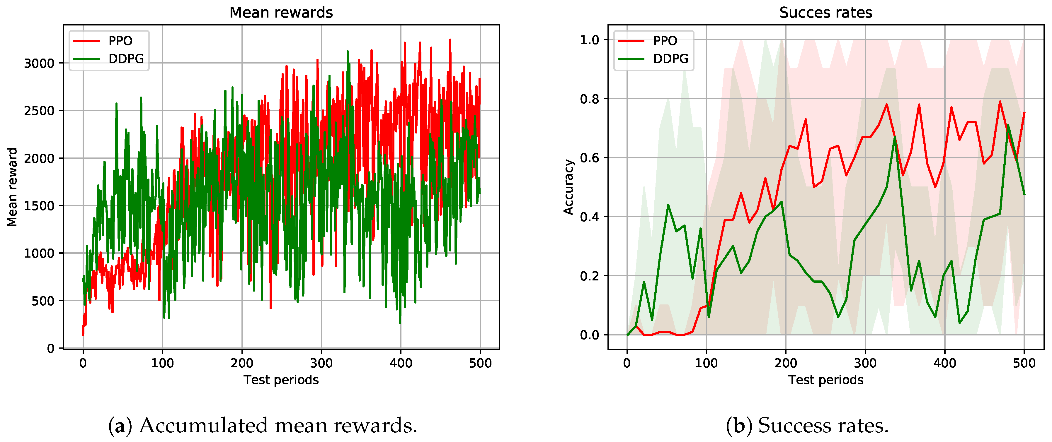
The goal of this test was to learn a low-level controller that could drive the mobile manipulator’s base close to the table, so that the arm could plan a trajectory up to the object. The learning process was carried out during 5M time-steps approximately, and an evaluation period was performed every 20 episodes. The results obtained with both PPO and DDPG algorithms are depicted in Figure 5. Figure 5a shows the mean accumulated rewards obtained in each of the 500 evaluation periods. The obtained success rates are depicted in Figure 5b. Due to the unstable nature of DRL algorithms, the obtained success rates vary considerably. Thus, to better understand the results, the mean value and the maximum/minimum values are shown per 10 test periods.

Concerning the accumulated mean rewards, DDPG converged faster than PPO but, when the learning process moved along, PPO obtained higher rewards. The fact that DDPG obtained higher initial rewards is explained by two main reasons: (1) The policy bounds the actions between −1 and 1 so that it is not penalised for high velocities. (2) From the initial learning steps, this algorithm predicts smooth velocity changes across consecutive time-steps and, thus, is not penalised for high accelerations. Instead, PPO does not bound the actions and that is why it is penalised for high velocities and accelerations in the initial learning steps. Nevertheless, this algorithm is able to understand that lower velocities/accelerations are not penalised and, once learned, it obtains higher rewards than DDPG.

Regarding the success rates, it can be seen clearly that DDPG approximated the goal faster than PPO. Although, in some evaluation periods, it succeeded 100% of the time, it presented an unstable behaviour. As explained before, PPO takes more time to approximate the goal but, when it learns to drive smoothly, it shows a more stable behaviour. Besides, it could get 100% success rate considerably more times than DDPG. Off-policy algorithms are said to be able to better explore the environment than on-policy algorithms. In our environment, due to the initial random poses and the limited work-space of the robot, the exploration problem decreased considerably. PPO is an on-policy algorithm and takes more time to explore the environment than DDPG and that is another reason DDPG approaches the goal faster than PPO. Nevertheless, PPO relatively quickly improves enough for its policy to be able to succeed.

DRL has been applied to goal reaching applications either in manipulation or in navigation. Typically, those goals are not surrounded by obstacles and this makes the learning process easier. In this case, the goal (the object) was on top of the table and the robot had to learn to approximate to it without colliding with the obstacle. The reward function defined in this test encouraged the robot approximating to the object as much as possible and the robot had to use the contact information to learn where the table was to not collide with it. Although an additional reward was given when the arm’s planning succeeded, it first tried to get as close as possible to the table, sometimes colliding with it and that is one of the reasons that caused the unstable behaviour of both algorithms.

Due to the variable pose of the object, in some episodes, if the object was near to table’s edge, it had the possibility to get closer, scoring higher rewards. In addition, the initial poses of both the robot and the object in every test period were totally random and thus the accumulated rewards and/or success rates varied considerably.

5.2. Test 2

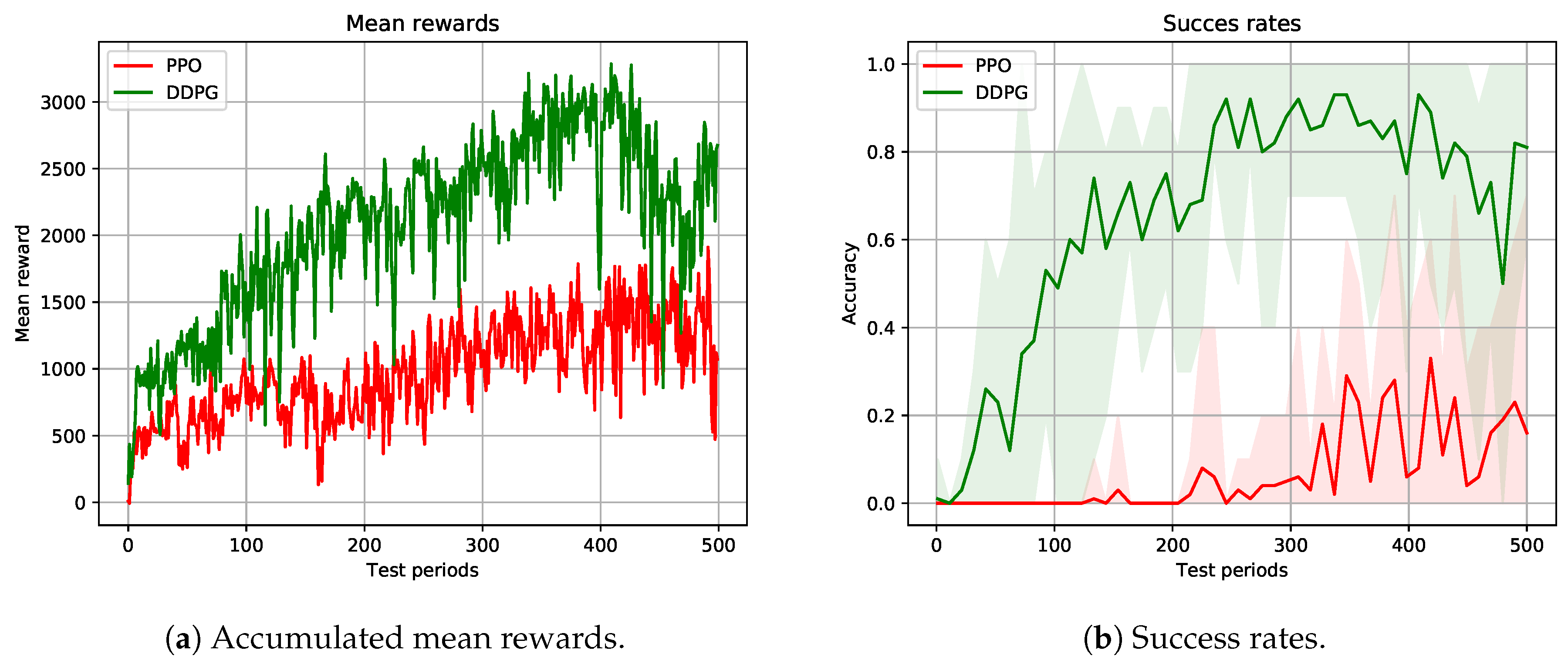
The goal of this test was to learn a low-level controller that could drive the mobile manipulator’s base close enough to the table for the arm to be able to plan a trajectory up to the object. In this case, a wall was placed near the object with the aim of making the decision making problem more difficult. The learning process was carried out during 2.5M time-steps and an evaluation period aws performed every 10 episodes. In Figure 6, the results obtained with both PPO and DDPG algorithms are depicted.

Concerning the accumulated mean rewards (Figure 6a), DDPG’s performance was better than PPO’s for the overall learning process. Due to the bounded actions and the smooth output of DDPG, it could get higher rewards in the initial learning steps. Thanks to the fact that this algorithm is off-policy, it is able to better explore the environment and, thus, it learns to locate the robot’s base much closer to the object than PPO. In addition, the constant pose of the box simplified the exploration problem, since the base always had to navigate to the same area of the environment and, consequently, the mean rewards were not as irregular as in the first test.

The success rates depicted in Figure 6b indicate that DDPG’s performance was much better than PPO’s, being the former able to score 100% success rate multiple times. DDPG could learn relatively quickly where the grasping zone is, discarding the poses over the wall. After navigating to the grasping zone, the learned policy stoped the robot sending near to zero velocities to the base. In addition, the deterministic behaviour of the algorithm enabled the robot to learn a more stable behaviour near the table, avoiding collisions. Even though PPO could learn to drive the robot near the correct grasping zone, it could not learn to stop it and continued sending velocities high enough to get the robot out of the grasping zone. Besides, due to the stochastic policy, the robot’s performance near the table was not as robust as DDPG’s, sometimes colliding with it.

6. Discussion and Future Work

In this work, we successfully implemented several DRL algorithms for learning picking operations using a mobile manipulator. It is shown that it is possible to use the arm’s feedback to learn a low-level controller that drives the base to such a place that the arm is able to plan a trajectory up to the object.

Two state-of-the-art DRL algorithms were applied and compared to learn a mobile manipulation task. Specifically, the arm planner’s feedback was used to learn to locate the mobile manipulator’s base. To the best of our knowledge, this is the first approach that uses the arm’s feedback to acquire a controller for the base.

Although DRL enables the learning of complex policies driven only by a reward signal, the unstable nature of those algorithms makes it difficult to obtain a robust behaviour. In addition, the sensitivity of DRL algorithms to hyper-parameters hinders finding the best parameter combination to get a robust and stable behaviour. Even though an optimisation over those hyper-parameters could be made, the large training times makes this process very expensive and commonly the default values proposed in the literature are used. Concerning the algorithms tested in this work, the results obtained show that the behaviour of the algorithms is dependant on several properties of the environment such as the state/action codification and the reward function definition. In addition, the network architecture used to encode either policies and the value-function has a large effect in the learning process. Even though the same network architecture and hyper-parameters were used in both tests, the results obtained are very different. Therefore, each environment needs the algorithm to be tuned in the best way to solve the problem, which is why the learned policies are not reproducible.

The reward function definition is another key point of the learning process, since it is entirely guided by this signal. A logical approach could be to give a reward to the robot in the last step only if the arm plans a trajectory, but, unfortunately, using only sparse rewards does not work well. In several goal reaching applications, either with arms or mobile bases, a distance dependant reward is proposed. In our application, this encourages the robot to navigate close to the object so the arm can plan a trajectory. After some tests, we saw that a nonlinear distance function accelerates the learning process.

Although DRL algorithms are typically trained in simulation, the experience acquisition is still the bottleneck of DRL based applications applied to robotics. Even though we accelerated the simulation, the entire learning process took several hours. Nevertheless, to be able to transfer the learned policy to a real robot and reduce the reality gap, the robot must be simulated accurately. Thus, a balance between simulation accuracy and training time acceleration should be found.

Moreover, it is complex to tune the algorithms to get a robust performance. We intend to increase the perception capabilities of the robot to be able to navigate in a more secure way and to be aware of the dynamical obstacles placed in the environment, using 2D/3D vision for example. Most of the applications in the literature map observations directly with low-level control actions and this black-box approach is not scalable. To be able to learn multiple behaviours and to combine them, hierarchical DRL proposes to learn a hierarchy of behaviours in different levels. In that vein, our goal is to learn a hierarchy of behaviours and, after training them in simulation, test those behaviours in a real robot.