Abstract
This study applies a decomposed method to determine adequate countermeasures against excessive fault current levels in power systems. A set of candidate locations for the countermeasures such as bus splitting and current limiting reactors are pre-defined and modeled using variable reactances. A decomposition method is applied for the decision-making on the selection of the location and type of countermeasures. The main problem is to identify the optimal settings of the variable reactances by considering the sensitivities of the bus fault currents and generation costs with respect to the incremental increase in the reactance values of each countermeasure. For the subproblem, the optimization tool of fuzzy fault level constrained optimal power flow (FFLC-OPF) is applied to obtain the optimal operating point for the system with the given reactance settings. The FFLC-OPF incorporates both traditional constraints and fault level constraints in solving for the power flow. In addition, illustrative examples using the modified 28-bus system are included to show the effectiveness of the decomposition method.
1. Introduction
Diverse concerns in terms of security arise in operating the modern power system. Operating points of the power system are frequently brought to the system’s operating limits [1]. This trend mainly comes from various reasons. One of them is the reduced system’s security margin by the competitive environment of modern electricity markets, and another reason is the usual compromise for new generation over system security investments resulting to stressed conditions of the system operation. Furthermore, system protective devices which are initially designed to meet the security needs of the old network are now subjected to increasingly unpredictable scenarios and therefore making it prone to malfunction. The trend seems to be more severe in those power systems with increased load and generation.
It is of paramount importance to achieve economic operation of the power system without violating the secure operating limits [2] such as thermal limits, voltage limits, and fault level limits. To efficiently obtain the solution for the problem, several formulation and solution techniques for optimal power flow (OPF) were proposed in the literatures [3,4,5,6]. The tool of OPF can be enhanced further to consider new operating limits for the secure operation of emerging power systems, and it is important to come up with the formulations for the specified OPFs and their solution techniques.
In the planning and operational planning stages for power systems, excessive fault current levels at some locations should be avoided using adequate countermeasures [7,8]. In the literature, there are several countermeasures for fault current security. When the expected fault currents are over the ratings of the corresponding circuit breakers (CB), the re-installation of circuit breakers with higher ratings is desirable. However, in the operational planning stage, that might not be viable, so other countermeasures are needed to be considered. Bus splitting and installing current limiting reactors (CLR) at critical lines are regarded as other options to maintain system operating limits [7]. This paper mainly deals with the problem of determining countermeasures against excessive fault currents in power systems using an optimization method.
Practically, line faults are mostly concerned in operation, and to evaluate the total fault current on the location, a dummy bus needs to be added in advance and bus fault currents are calculated. When it comes to line faults, one of important issues is how to locate faults. In [9], a fault location method based on traveling wave principle was developed and applied to BC Hydro 500 kV networks. The fault location algorithm in [10] employed Thévenin equivalents using measured voltage and current information at both sides of the faulty line. In [11], a direct method based on three phase circuit analysis for unbalanced distribution systems was proposed. However, when making decision on countermeasures against excessive fault currents, bus fault currents in the study area are determined for fault levels in the operational planning stage, because it is to come up with countermeasures to cover severest conditions.
In [12,13], the formulation by fault level constrained optimal power flow (FLC-OPF) was proposed. It was proposed to take into account the limits of protective devices. The FLC-OPF method directly incorporates the constraints of expected fault currents in the OPF. The primary purpose of this specified OPF was to determine the optimal locations and capacities of new generators that would not violate the existing network and fault level constraints. The advantage of the direct inclusion of fault level constraints in the optimal power flow is that shadow costs are produced, connecting the overall optimum of the objective function with operational and fault current constraints. Furthermore, this feature could also be used in the design of a reinforcement planning mechanism, which would assess the return of investments on both network and protection equipment. In [14], an allocation method of fault current limiters using OPF with fault current level constraints was proposed.
However, because of the crisp fault current constraints, some optimal solutions might not be achieved in some scenarios. In [15,16], network reconfigurations algorithm were proposed to reduce the expected fault currents in the power system. The network reconfiguration algorithm allowed countermeasures such as bus splitting and transmission line opening. The manipulation of the network topology might cause the reduction of fault currents allowing the satisfactions of CB limits and causing the method to eventually converge at an optimal solution. However, for the cases where the system’s initial condition have critically excessive fault current levels and the resource set of countermeasures is not enough to cover the initial fault current violation, the network reconfiguration algorithm might not be able to provide a set of feasible solutions. Fuzzy-based approaches in solving allocation and control problems in power systems are proven to be robust [17,18]. This paper adopts the fuzzy set theory to deal with the fault level constraints (FLCs) for the systems with critically excessive fault current levels. By applying the fuzzy enforcement [19,20,21] to the FLC-OPF, slight violations in the fault level constraints can be allowed to achieve adequate solutions even though there are not enough resources for reducing the fault current levels.
The purpose of this paper is to formulate and test a method that would aid in the decision-making of which countermeasure such as bus splitting and/or CLR will be applied to reduce the fault current level of the network. Consequently, given the set of pre-defined candidate locations for the two countermeasures, the optimal location and allocation of reactance values are determined. Furthermore, to model the two kinds of countermeasures at the same time, variable reactances are inserted on the candidate locations. In this paper, a decomposition method is employed for the purpose of simultaneously considering both countermeasures, while the variable reactances are the decision making variables. In the subproblem of this decomposition method, the optimization tool of fuzzy fault level constrained optimal power flow (FFLC-OPF) is performed to acquire the optimal operating point with the given network topology considering both traditional constraints and fault level constraints. On the other hand, the main problem is done to identify the optimal settings of the variable reactances for the countermeasures considering sensitivities of fault currents and generation costs with respect to the incremental of each reactance. These two problems are iteratively solved until the convergence tolerance in terms of fault current violations from the given FLCs is reached. This paper provides illustrative examples in applying the decomposition method to the modified 28-bus system.
The main features of the proposed method are (i) the use of a decomposed approach for determining adequate countermeasures and an OPF operating point that is within fault current levels, (ii) that of two types of fault current countermeasures such as bus splitting and current limiting reactors, (iii) that of FFLC-OPF that incorporates both traditional constraints and fault level constraints in solving for the power flow as well as the application of fuzzy concept to the FLCs that enhances the search for feasible solutions, and (iv) that of sensitivity analysis in determining which countermeasure contributes to the decrease of fault current levels.
2. Fuzzy Fault Level Constrained Optimal Power Flow (FFLC-OPF)
2.1. Fuzzy Fault Level Constraints
Fault current levels in the system should be within the breaking duties of circuit breakers (CBs). Several parameters in terms of fault current security are needed to be checked, but this paper focuses on initial symmetrical fault currents which can be used in the stage of operational planning. To obtain initial symmetrical fault currents for a 3-phase short circuit fault at a faulted bus i, the following formulation is usually used:
where is the pre-fault voltage at the faulted location. In Equation (1), represents the diagonal components of the bus impedance matrix or the driving point impedance. When the fault current level exceeds the corresponding CB’s rating, the faulted location cannot be isolated from the unaffected system and hence the fault can spread throughout the system and the affected region can be enlarged. Thus it is really important to maintain the fault current level within the CB’s rating. This can be explained with a constraint, which is called a fault level constraint (FLC), as follows:
where is for the CB’s breaking duty. In other words, the CB’s breaking duty is the FLC in that specific bus.
Assuming that FLCs are included in an optimization formulation and available control measures to reduce fault currents at critical locations, some of the FLCs might be violated and this can cause infeasibility of the optimization problem. For that reason, this paper comes up with the application of fuzzy concept to FLCs. For the purposes of this study, a triangular fuzzy membership function is introduced to define the fuzzy membership set as seen in Figure 1. This technique is called fuzzy enforcement, and this application can adequately deal with variables that slightly exceed their limits. In this paper, the technique of fuzzy enforcement is applied to FLCs, so that even when the initial condition of the system violates FLCs, the optimizer can provide the optimal solution.
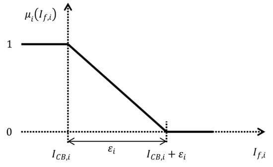
Figure 1.
Triangular fuzzy membership function of a fault level constraint.
The triangular membership function in Figure 1 can be expressed mathematically as follows:
where stands for the acceptable limit of fault current violation for bus during the solution process. The triangular fuzzy membership function represents a degree of certainty for each member.
2.2. Formulation of FFLC-OPF
Basically, OPF is an algorithm that determines the optimal dispatch of active power generation in the system and other parameter settings that meets the load demand and satisfies the feasibility within the operating limits. The state variables of the system are the voltage magnitude and the voltage phase angle at each bus. Active and reactive power injection, which are functions of the state variables, need to be balanced with the difference between generation and demand. The active and reactive power balance equations for each bus are expressed briefly as follows:
where and denote active and reactive power, respectively, and stand for the vectors for bus voltage magnitude and angle, respectively. In Equation (4), subscripts , , and stand for injection, generation and demand, respectively.
Additionally, the system’s operating limits need to be incorporated into OPF with the form of inequality constraints and they are formulated as follows:
where is apparent power flow on the branch connecting bus and . In Equation (5), and are the lower and upper limit of bus voltage angle at bus ; and are the lower and upper limit of the bus voltage magnitude; and are the lower and upper limit of the active power generation at bus i; and are the lower and upper limit of the reactive power generation at bus ; and are the lower and upper limit of apparent power flow of the branch to .
To include FLCs in the OPF, the magnitude of the fault current rather than its complex value is needed. The fault current of each bus and its corresponding upper limit is needed to be considered as in Equation (2). As in Equation (3), in this paper, a fuzzy membership function is applied to each FLC to properly deal with the initial infeasibility and the situations wherein the control measures are not enough to get a feasible solution. Instead of crisp constraints, the fuzzy FLCs are incorporated as follows:
where is the acceptable tolerance for fault current that will exceed the . Also, the value of the fuzzy membership function for the FLC of the faulted location is represented as . This membership function value is taken into account in the formulation of the algorithm’s objective function. In the FFLC-OPF, the augmented objective function should be used as follows:
where is the number of generators in service and is the number of fault current limits in the problem. The objective function in Equation (7) of the FFLC-OPF minimization problem consists of the summation of the generators’ cost functions and a secondary term containing the lower limit of the membership functions for FLCs. For the first term, the quadratic cost functions of the generators are used in this study, so in Equation (7), denotes the cost function for generator, . The second term is the product of a weighting factor , and the lowest value among the membership functions for the set of FLCs. As mentioned in the previous subsection, the value of the membership functions can range from 0 to 1. The value of the second term needs to be as close to the first term, so the value of is selected near the value of the first term. This formulation ensures that the feasible solution that can be obtained has the least FLC violations because of excessive fault currents.
3. Decomposition Method for Countermeasures against Excessive Fault Currents
3.1. Motivation
The increase in the load demand consequently results to increased levels of fault current that might exceed the breaking duty of CBs in the credible operating point. The critically excessive fault current levels can disrupt the proper operation of CBs, and hence they can lead to a widespread low voltage problem caused by sustained or permanent failures in some components in the system. The aim of this paper is to reduce the fault currents through applying bus splitting and installing CLRs in the power systems while keeping the fault current levels within the CB breaking duties. The countermeasures are not incorporated in the formulation of the FFLC-OPF in the previous section.
Several countermeasures can be implemented against excessive fault current levels, as in [22,23,24]. This paper concentrates on bus splitting and equipping CLR. The implementation of them can basically change fault current levels at the applied locations and neighboring buses. In addition, it is desirable to consider the two types of countermeasures at the same time in the decision making process because both of them need to be considered in the operational planning procedure and their applications affect each other. However, the two types of countermeasures might degrade the operational efficiency of transmission systems in terms of system loss and transient stability because of the increase of electrical distances between local generators and the external system. Thus it would be better to minimize the number of bus splitting locations and CLRs equipped in the system. For the purpose, then, a certain tool is needed for the optimal allocation of the countermeasures ensures adequate level of fault current reduction as well as system operational efficiency.
This paper adopts a decomposed approach to tackle the problem of decision making on bus splitting and equipping CLRs. Decomposition methods can be used for a complicated optimization problem which can be divided into a main problem and a subproblem. Decomposing the problem of application of appropriate countermeasures, in the paper, facilitates to deal with the discretized characteristic of them. The main decision variables of the original problem are integers. In the case of bus splitting, the variables are binary; in the case of placement of CLRs, they are also discrete values with a step increase of the reactance. The main problem is to decide whether to apply bus splitting and to install CLRs that would reduce fault currents further. That is, the main problem obtains the correction of the decision making variables. The subproblem is to evaluate the system operational efficiency in terms of fault current levels with the given decision variable settings from the optimal solution to FFLC-OPF. The main problem and subproblem are repeatedly performed until the final solution is obtained.
3.2. Main Problem
Instead of direct dealing with discrete main decision variables for bus splitting and CLRs, this paper adopts a way of modeling them by inserting continuous or intermediate reactances as shown in Figure 2. At the final stage of the main problem process, the solution needs to be discretized. The concept of the inserted reactance for bus splitting was originally proposed in [16], and it can be extended for current limiting reactors.
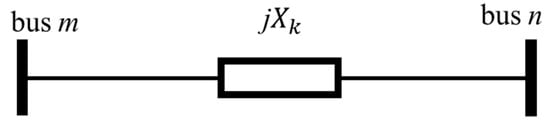
Figure 2.
Inserted X variable for bus splitting and current limiting reactor installations.
The formulation of the main problem can be expressed as follows:
where and denote the reactance at the k-th candidate location and its initial value. In Equation (8), and are the total number of candidate locations and fault level constraints, respectively; stands for the sensitivity of the fault current at bus i with respect to the change of the value of ; is the fault current level at bus i for every change in is the breaking duty of CB at bus i; and and are the lower and upper limit of . Lastly, is the acceleration coefficient. From the above formulation, one can notice that in the main problem the variables are determined to satisfy the CB limits of the FLCs, minimizing the deviation from their initial values.
As mentioned above, the aim of this paper is to deal with the two types of fault current countermeasures at one formulation and they are initially modeled with continuous reactances at candidate locations. In the case that the decision of main problem is made only by sensitivity information, it might cause infeasibility of constraints or a large increase in objective function values when applying the new X settings by main problem. The reason is that there exist nonlinear effects of transmission branch parameters. The nonlinearity in terms of branch parameter variations was investigated in [25]. In the preliminary simulation results of this paper, it was also noticed that there were some cases where inadequate settings of s from the main problem caused infeasibility such as divergence of the subproblem with FFLC-OPF. Therefore, such a way to prevent those infeasible situations need to be implemented, and it is done by modifying the sensitivity of the reactance causing a rather large change in the generation cost or infeasibility. The modified formulation of the sensitivity of i-th FLC with respect to the change in the k-th reactance () for the corresponding candidate countermeasure is as follows:
where denotes the change in fault current with respect to and is the binary variable representing whether to apply the -th candidate as a countermeasure. In addition, the binary variable, , is chosen by observing the change of the generation cost by OPF before solving the main problem as follows:
where is the threshold value of generation cost increase and NG is the total number of generators. In Equation (10), represents the change in the total generation cost after the calculation of OPF with the new value of . Using Equations (8)–(10), the recommended correction of X’s in the main problem can avoid rather large difference of generation cost or divergence of subproblem.
In the main problem, the s for candidate locations are intermediate, but in the final decision making, they should be discretized into , , and , because of their discrete features of bus splitting and CLRs in real application. The settings used in this paper are shown in Table 1. Since there are two countermeasures being considered in the problem, one set of discrete reactance values was considered for CLR and another one for bus splitting. The incremental increase, , in the reactance values for sensitivity calculation is 0.01 [pu]. Discrete additional reactance values for CLRs are 0.10 [pu]. And the discretized reactance values for bus splitting is either 0.0001 [pu] or 10 [pu] to represent a split or integrated bus, respectively. To discretize the continuous or intermediate reactances, a simple rounding method is used.

Table 1.
Parameter setting example for discretization. CLR: current limiting reactors.
3.3. Overall Procedure of the Proposed Method
The overall procedure of the proposed method is as follows, with Figure 3:
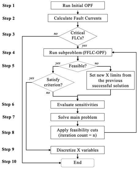
Figure 3.
Flowchart of the overall procedure. OPF: optimal power flow; FLCs: fault level constraints; FFLC-OPF: fuzzy fault level constrained optimal power flow.
- Step 1
- An initial OPF is done on the network base case.
- Step 2
- Bus fault currents are calculated.
- Step 3
- Fault currents are compared to the given upper limits of FLCs to identify the critical locations with excessive fault currents. The algorithm proceeds to the next step when there is a critical FLC that violates the CB limit; otherwise, the algorithm stops.
- Step 4
- The subproblem is solved by running the FFLC-OPF on the network.
- Step 5
- If the FFLC-OPF finds a feasible solution, the z value or the least among the FLC membership function values is checked if within the following stopping criterion:where is the tolerance of convergence equal to 0.01. If the stopping criterion is not satisfied, the algorithm proceeds to Step 6; otherwise, it goes to Step 8. On the other hand, if the FFLC-OPF cannot find a feasible solution, the previous variable limit that yielded a feasible solution is set as the maximum limit before the algorithm proceeds to Step 6.
- Step 6
- The sensitivities w.r.t. s using Equation (9) are evaluated.
- Step 7
- The main problem is solved to determine the main decision variables ( variables) that will remove (or reduce) the FLC violations. Subsequently, this network with new variables is passed on to the next step.
- Step 8
- The new set of variables is used as additional set of constraints such as in Equation (8c).
- Step 9
- The variables are discretized by simply rounding the intermediate values to the nearest reactance values that represents bus splitting and additional CLRs. This is the final output of the algorithm.
- Step 10
- The process stops.
In this paper, FFLC-OPF for the subproblem was implemented on the OPF module in MATPOWER [26], and it was chosen because of its extensible structure for a specified purpose with OPF. In addition, KNITRO solver was used to solve the AC OPF portion of the algorithm. Basically the proposed decomposition method is to the nonlinear optimization problem including binary and discrete decision variables, and obviously those variables have nonlinear effects on equality and inequality constraints. That is, there might be several local optima other than the solution of the proposed method, but it can provide practical solutions with the least deviation from the original network.
4. Numerical Examples
The proposed algorithm of this paper was tested on a modified 28-bus network as shown in Figure 4. The said network was derived from the sample case network in [27]. In Figure 4, there are six bus pairs with bus splitting, and twelve bus pairs with CLR pre-defined candidate locations. The decomposition method was applied to this medium-sized test system to determine the correct locations for the countermeasures. Table 2 shows the impedances and ratings of the respective generators. These values are inputs needed for the fault current calculations. The coefficients and constant term for each generator quadratic cost function are listed in Table 3. Furthermore, the list of bus pairs with bus splitting and CLR countermeasures are shown in Table 4.
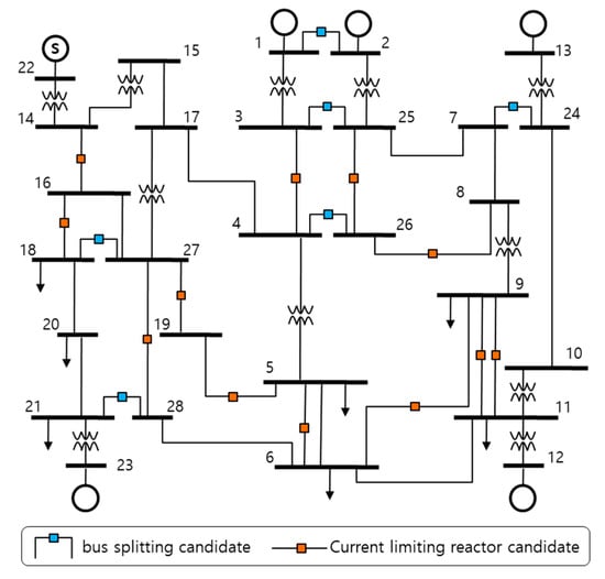
Figure 4.
Modified 28-bus network.
Table 2.
Generators’ impedances with the machine bases.
Table 3.
Generators’ quadratic cost function coefficients.
Table 4.
Candidate locations for countermeasures.
At each candidate location, a reactance was inserted between two bus pairs to represent a countermeasure. These continuous reactances (Xk) are the main variables in the decision making as described in Equation (8a). In addition, the range of minimum to maximum values for the reactance representing bus splitting (XBS) is 0.0001 to 10.000 [pu], while the reactance for CLR (XCLR) is 0.0001 to 0.3000 [pu]. In this simulation, two cases with different number of FLCs were tested. Case 1 deals with a network with three FLCs and Case 2 has twenty-six FLCs.
4.1. Case 1
In this section, a simple case was applied to test the functionalities of the algorithm. Three FLCs were selected and added as constraints to the FFLC-OPF. These FLCs are included to limit their corresponding bus fault currents levels. In this simulation, the FLC is the assigned maximum CB breaking duty () for each bus. The set of FLCs for Case 1 is listed in Table 5. Also, the acceptable limit of bus fault current violation () for the fuzzy membership function of each FLC is uniformly set as 20 [pu] for all three buses.
Table 5.
Circuit breaker limits in Case 1.
After executing the initial steps of the procedure in Section 3.3, the three FLCs were identified to be critical. Although the FFLC-OPF subproblem was able to find a feasible solution the calculated bus fault current levels in all three buses still exceeded their corresponding FLCs as listed in Table 6. The most excessive of the three fault current levels is at bus 1 which was 12.21% above its ICB,max which is 50 [pu]. Consequently, bus 1 has the lowest value among the three membership functions with 0.695. Buses 26 and 28 have better membership function values of 0.738 and 0.835, respectively. As stated in Equation (3), a value of 1.0 indicates a fault current level that is less than or equal to the ICB,max. Furthermore, since z is the value of the lowest membership function among the given set of FLCs, the algorithm’s stopping criterion is set such that all FLCs are satisfied Equation (11).
Table 6.
Fault current level at each iteration.
To further reduce the fault current levels at the three critical buses, adequate countermeasures should be applied to the existing network. The algorithm proceeds to Step 6, wherein the sensitivities of each critical fault current level with respect to the countermeasures in Table 4 are evaluated. The sensitivities in Equation (9b) was calculated using an increment of 0.01 [pu] for the variables ( Table 7 shows the FLC sensitivities with respect to the incremental increase in the variables particularly variables. For this case, the localized nature of the FLCs at buses 1, 26, and 28 resulted to negligible sensitivity values with respect to variables and were excluded in the Table 7. The sensitivity matrix also reflects the impact of each variables to the fault current levels at the FLC buses. Note that the negative value indicates a reduction in fault current level as modeled in Equation (9b). Hence, the FLCs at bus 1, 26, and 28 are more sensitive to the incremental increase in , and , respectively for this particular iteration.
Table 7.
Sensitivities with respect to the variables.
Afterwards, the algorithm proceeds to Step 7 where the main problem of minimizing the sum of all variables is solved Equation (8a). The sensitivity matrix from the previous step is utilized as part of the formulation of constraints for this linear programming problem Equation (8b). The sensitivity matrix, which is essentially the rate of change in fault current levels, multiplied by the optimal minimum set of variables must be less than or equal to the product of an acceleration coefficient ( 2.50) and the difference of its circuit breaking duties and existing fault currents. Table 8 shows the intermediate values of the variables after running the main problem. The calculated fault current level after the first iteration is shown in the third column of Table 6. Subsequently, the algorithm returned to Step 4 to run the FFLC-OPF to get a feasible operating point after the addition of the new variables from the first iteration.
Table 8.
X variables of each bus splitting candidate (Case 1). MFCC-OPF: modified fault current constrained optimal power flow.
The final fault current levels are shown in the last column of Table 6. Obviously, since all fault current levels are now below their , the least membership function is now equivalent to 1.0 and has satisfied the algorithm’s stopping criterion. The next step is to discretize the variables that were identified to cause the reduction of the fault current level of the network. Since the algorithm only took one complete iteration of the subproblem and main problem, the intermediate values are quite low. However, these intermediate values still indicate its effect on the identified FLCs that we aim to satisfy. In Table 8, variables with intermediate values are discretized and assigned with 10.0 [pu] for bus splitting. For comparison, the result applying the modified fault current constrained optimal power flow (MFCC-OPF) to the case with bus splitting candidates was shown in the last column of Table 8. MFCC-OPF adopted a soft-discretization technique within the solution procedure, and it is only applicable to the decision making on bus splitting and line opening The result of MFCC-OPF was the same as that of the proposed method.
Figure 5 below shows the initial and ICB,max fault current levels of each of the three buses with FLCs. Also shown in the graph are the effects on the fault current levels when countermeasures are applied on the network. From Table 8, priority in bus splitting countermeasures can be ranked according to their corresponding intermediate values: , , and . The countermeasure corresponds to splitting buses 21–28 and resulted to a fault level reduction in bus 28. Applying two bus splitting countermeasures involved and which resulted to a fault reduction in buses 28 and 1. Lastly, three bus splitting countermeasures resolved all excessive fault current levels in all three FLC buses.
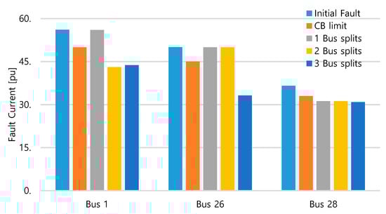
Figure 5.
Fault currents at each of the three FLC buses after applying countermeasures in Case 1.
4.2. Case 2
For this case, the proposed algorithm is tested using the same number and types of countermeasures from Table 4 but with more constraints than Case 1. Twenty-six FLCs are implemented in this simulation and the list of maximum CB breaking duties (ICB,max) is shown in Table 9. The goal of the proposed algorithm is to find a feasible solution that has the optimal type and allocation of countermeasure/s that would reduce the bus fault current levels within the FLCs which is the maximum CB breaking duties for each bus.
Table 9.
Circuit breaker limits in Case 2.
Similar with the previous case, all the initial fault current levels at the FLC buses exceed their corresponding ICB,max. The worst of which is at bus 27 that initially exceeds its ICB,max by 13.02% giving it the least membership function value of 0.772 as shown in Figure 6. In this case, the FLC buses are scattered throughout the network, therefore each incremental increase in the variables have varied effects on the fault current level calculations of each bus. To be able to reduce the fault current level in a wider scale, the sensitivity matrix must reflect which reduces the most bus fault current levels. The size of the sensitivity matrix for this case is twenty-six FLCs by eighteen variables. As discussed in Section 3.2, there were variables that were identified to be causing a rather large change in the generation cost and were causing infeasible solutions on the subproblem. In Case 2, it was identified that any increase in the settings of three variables namely, , and caused the divergence on the subproblem with twenty-six FLCs. The modified Equations (9a) and (10) were implemented so the sensitivity values of the FLCs from these variables were set to zero.
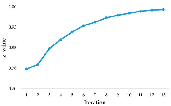
Figure 6.
Least membership functions value at each iteration Case 2.
Figure 6 shows the trajectory of the z values on each run. After 13 iterations within 50.34 seconds, the stopping criterion was satisfied. Also, the trajectories of the variables for all iterations are shown in Figure 7 and Figure 8. In Figure 7, only and have intermediate values which means that the incremental increase in the reactances of these bus splitting pairs contributed on the reduction of the fault current levels on the system. Both variables are considered for bus splitting while the other four bus pairs are kept integrated as indicated by the discrete points in Figure 7.
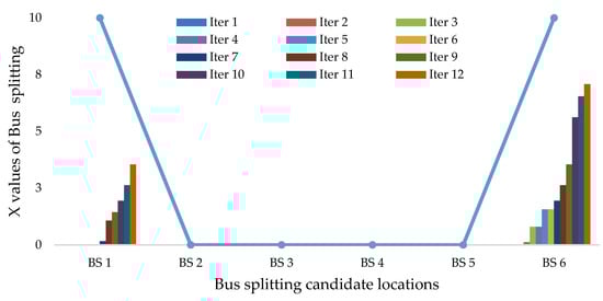
Figure 7.
Set of Bus splitting variables at each iteration in Case 2.
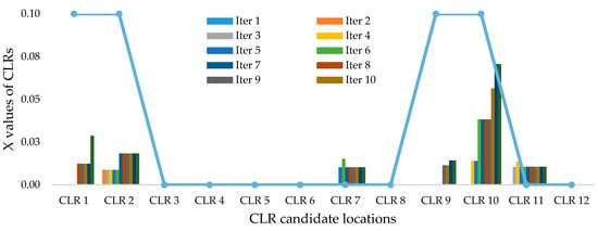
Figure 8.
Set of CLR variables at each iteration in Case 2.
During the simulation, there are also some instances wherein the subproblem diverges because of an variable that reaches a reactance value after some time which results to an infeasible solution. Whenever this happens, Step 5 of the algorithm sets the previous variables that yielded a feasible solution as the maximum limit before the algorithm proceeds to Step 6. In this way, the main problem algorithm can search for other feasible solutions for the decision variables. This instance is illustrated in Figure 8 wherein increased in value and resulted to divergence during the fourth iteration, and with during the sixth iteration. Both variables were limited to their previous variable values during Step 5 of their respective iterations.
Similarly, Figure 8 shows the intermediate values of the twelve variables per iteration. The graph shows that the FLCs were sensitive to the incremental increase of only six variables most especially with that reached a value of 0.0707 [pu] on the 13th iteration. All variables with intermediate values are considered as an additional 0.1 [pu] CLR countermeasures except for and variables since further increase in their values causes divergence on the subproblem. The discretization of variables is illustrated in Figure 8.
In summary, the list of variables that were considered as bus splitting and CLR countermeasures for Case 2 is shown in Table 10. The variables are also ranked based on their intermediate values and were applied on the network in the order as they were ranked. As seen in Figure 9, there is a general improvement in the z value as the number of applied countermeasures was increased. Also, the trend shows that applying one countermeasure and two countermeasures resulted to the same membership function. As discussed earlier, the z value is the least membership function in the given set of FLCs and this reflect the FLC bus with the highest excessive fault current level violation. Applying one and two bus splitting countermeasure have different effects on the fault current levels of different buses. However, in this specific case, a bus split between buses 21–28 and an additional bus split in buses 1–2 did not affect the fault current level at bus 27 which remained at 38.48 [pu] yielding a membership function value of 0.8258 in both applications. A deeper look at the data revealed that the fault current level at bus 27 was significantly reduced after the application of CLR2 and CLR9, where additional 0.1 [pu] reactances were inserted between bus pairs 5–19 and 25–26, respectively. Almost a similar incident happened between applying five and six countermeasures as seen in Figure 9.
Table 10.
X variables of the bus splitting and CLR candidates (Case 2).
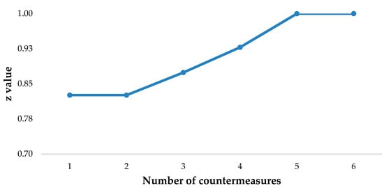
Figure 9.
Countermeasures and their corresponding least membership function values.
Applying six countermeasures resulted to more reduction on the fault current levels at the FLC buses compared to only applying five countermeasures, except at bus 7 where six countermeasures only reduced the fault current level by 0.003 [pu]. This explains the very minimal improvement on the z value between the application of five and six countermeasures. In addition, it is important to note that all of these countermeasures and their combinations resulted to feasible solutions to the FFLC-OPF. Ultimately, all twenty-six FLCs were satisfied after the application of the two bus splits (BS6 and BS1) and four current limiting reactors with 0.1 [pu] (CLR10, CLR1, CLR2, and CLR9). This is reflected with a z value equivalent to 1 as shown in Figure 9. Also, worth nothing that applying five countermeasures (BS6, BS1, CLR10, CLR1, and CLR2) is a good solution as well since it adequately satisfied the FLCs and has a z value of 0.9999. Lastly, the initial fault current levels and the fault current levels after the application of the six countermeasures are illustrated in Figure 10. Notice that all resulting fault current levels were reduced and are now within the maximum CB breaking duties. From an average initial fault current level excess of 5%, applying the six countermeasures resulted to a fault current level average of 12.85% reduction below CB limits in the twenty-six FLC buses.
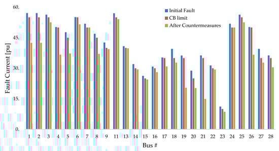
Figure 10.
Fault current levels before and after applying the six identified countermeasures in Case 2.
5. Conclusions
This paper presents a decomposed approach in determining adequate countermeasures for excessive fault current levels. The installation of current limiting reactors and bus splitting countermeasures are modeled as reactance variables, while the CB breaking duties are considered as the fault level constraints on the buses. The main problem of this method is the calculation of the minimum amount of reactance variables while the fault current level sensitivities are taken into account. The subproblem in this method is a Fuzzy Fault Level Constrained Optimal Power Flow which considers traditional OPF constraints and additional fault level constraints. The FFLC-OPF solves for a feasible operating point of the system after the application of the selected countermeasures from the main problem. The algorithm was tested on a medium-sized network and was proven to solve for an optimal set of countermeasures that satisfied multiple fault level current constraints throughout the network without compromising the feasibility of operation. The fuzzy treatment for the additional fault level constraints assigns a membership function on fault currents that exceeds the CB breaking duties. As a result, the ability of a set of countermeasures to reduce the fault current levels is reflected on the resulting fuzzy membership function. The decomposition of the problem allows the main problem to consider two countermeasures at the same time, while the subproblem preserves the feasibility of solution for every set of additional reactances at each iteration. The decomposed approach of solving the OPF and reactance values provide a better way of solving the problem by solving for minimum number of countermeasures without compromising the feasibility of operation.
Author Contributions
B.-H.F. designed the research, implemented the algorithm, conducted simulations and wrote the paper. H.S. conceived the study, improved the theoretical part and supervised the research.
Acknowledgments
This work has been supported by Seoul National University of Science & Technology.
Conflicts of Interest
The authors declare that there is no conflict of interests regarding the publication of this paper.
References
- Wood, A.J.; Wollenberg, B.F.; Sheblé, G.B. Power Generation Operation and Control, 3rd ed.; Wiley & Sons: Hoboken, NJ, USA, 2014. [Google Scholar]
- Stott, B.; Alsac, O.; Monticelli, A.J. Security analysis and optimization. Proc. IEEE 1987, 75, 1623–1644. [Google Scholar] [CrossRef]
- El-Hawary, M.E. Optimal Power Flow: Solution Techniques, Requirements, and Challenge; IEEE Publication: Piscataway, NJ, USA, 1996. [Google Scholar]
- Momoh, J.A.; Koessler, R.J.; Bond, M.S.; Stott, B.; Sun, D.; Papalexopoulos, A.; Ristanovic, P. Challenges to Optimal Power Flow. IEEE Trans. Power Syst. 1997, 12, 444–447. [Google Scholar] [CrossRef]
- Stott, B.; Alsac, O. Optimal Power Flow-Basic Requirements for Real-Life Problems and Their Solutions. Available online: http://www.ieee.hr/_download/repository/Stott-Alsac-OPF-White-Paper.pdf (accessed on 24 April 2018).
- Zhu, J. Optimization of Power System Operation, 2nd ed.; John Wiley & Sons, Inc.: Hoboken, NJ, USA, 2009. [Google Scholar]
- Mahmoudian, A.; Niasati, M.; Khanesar, M.A. Multi objective optimal allocation of fault current limiters in power system. Electr. Power Energy Syst. 2017, 85, 1–11. [Google Scholar] [CrossRef]
- Vasilj, J.; Sarajcev, P.; Goic, R. Modeling of current-limiting air-core series reactor for transient recovery voltage studies. Electr. Power Syst. Res. 2014, 117, 185–191. [Google Scholar] [CrossRef]
- Lee, H.; Mousa, A.M. GPS travelling wave fault locator systems: Investigation into the anomalous measurements related to lightning strikes. IEEE Trans. Power Deliv. 1996, 11, 1214–1223. [Google Scholar] [CrossRef]
- Takagi, T.; Yamakoshi, Y.; Yamaura, M.; Kondow, R.; Matsushima, T. Development of a new type fault locator using the one-terminal voltage and current data. IEEE Trans. Power Appar. Syst. 1982, PAS-101, 2892–2898. [Google Scholar] [CrossRef]
- Choi, M.-S.; Lee, S.-J.; Lee, D.-S. A new fault location algorithm using direct circuit analysis for distribution systems. IEEE Trans. Power Deliv. 2004, 19, 35–41. [Google Scholar] [CrossRef]
- Vovos, P.; Harrison, G. Optimal Power Flow as a Tool for Fault Level Constrained Network Capacity Analysis. IEEE Trans. Power Syst. 2005, 20, 734–741. [Google Scholar] [CrossRef]
- Vovos, P.; Bialek, J. Direct Incorporation of Fault Level Constraints in Optimal Power Flow as a Tool for Network Capacity Analysis. IEEE Trans. Power Syst. 2005, 20, 2125–2134. [Google Scholar] [CrossRef]
- Khazali, A.; Kalantar, M. Optimal power flow considering fault current level constraints and fault current limiters. Electr. Power Energy Syst. 2014, 59, 204–213. [Google Scholar] [CrossRef]
- Vovos, P.N.; Song, H.; Cho, K.W. A Network Reconfiguration Algorithm for the Reduction of Expected Fault Current. In Proceedings of the 2013 IEEE PES General Meeting, Vancouver, BC, Canada, 21–25 July 2013. [Google Scholar]
- Song, H.; Vovos, P.N.; Cho, K.W.; Kim, T.S. Decision Making on Bus Splitting Location Using a Modified Fault Current Constrained Optimal Power Flow. J. Electr. Technol. 2016, 11, 76–85. [Google Scholar] [CrossRef]
- Ramadan, H.A.; Wahab, M.A.A.; El-Sayed, A.M.; Hamada, M.M. A fuzzy-based approach for optimal allocation and sizing of capacitor banks. Electr. Power Syst. Res. 2014, 106, 232–240. [Google Scholar] [CrossRef]
- Vigneysh, T.; Kumarappan, N. Grid interconnection of renewable energy sources using multifunctional grid-interactive converters: A fuzzy logic based approach. Electr. Power Syst. Res. 2017, 151, 359–368. [Google Scholar] [CrossRef]
- Song, H. Fuzzy-Enforced Complementarity Constraints in Nonlinear Interior Point Method-Based Optimization. Int. J. Fuzzy Log. Intell. Syst. 2013, 3, 171–177. [Google Scholar] [CrossRef]
- Liu, W.H.E.; Guan, X. Fuzzy constraint enforcement and control action curtailment in an optimal power flow. IEEE Trans. Power Syst. 1996, 11, 639–644. [Google Scholar] [CrossRef]
- Zimmerman, H.J. Fuzzy Set Theory and Its Application; Kluwer: Norwell, MA, USA, 1985. [Google Scholar]
- Tleis, N. Power Systems Modelling and Fault Analysis: Theory and Practice; Newnes: Oxford, UK, 2008.
- Anderson, P.M. Analysis of Faulted Power Systems; Wiley-IEEE Press: Hoboken, NJ, USA, 1995. [Google Scholar]
- Andersson, G. Modelling and Analysis of Electric Power Systems; ETH Zurich: Zürich, Switzerland, 2008. [Google Scholar]
- Flueck, A.J.; Dondenti, J.R. A new continuation power flow tool for investigating the nonlinear effects of transmission branch parameter variations. IEEE Trans. Power Syst. 2000, 15, 223–227. [Google Scholar] [CrossRef]
- Zimmerman, R.D.; Murillo-Sanchez, C.E.; Thomas, R.J. Matpower: SteadyState Operations, Planning and Analysis Tools for Power Systems Research and Education. IEEE Trans. Power Syst. 2011, 26, 12–19. [Google Scholar] [CrossRef]
- Power Technologies International. PSS/E 31.0 Users Guide; Siemens PTI: Schenectady, NY, USA, 2007. [Google Scholar]
© 2019 by the authors. Licensee MDPI, Basel, Switzerland. This article is an open access article distributed under the terms and conditions of the Creative Commons Attribution (CC BY) license (http://creativecommons.org/licenses/by/4.0/).