Coordinated Control of Multiple Euler–Lagrange Systems for Escorting Missions with Obstacle Avoidance

Abstract

This study investigates the coordinated control problem of Euler–Lagrange systems with model uncertainties in environments containing obstacles when escorting a target. Using an outer–inner loop control structure, a null-space-based behavioral (NSB) control architecture was proposed in the outer loop considering obstacles. This architecture generates the desired velocity for the inner loop. The adaptive proportional derivative sliding mode control (APD-SMC) law was applied to the inner loop to ensure fast convergence and robustness. All the robots were distributed around the target evenly and escorted the target at a specified distance while avoiding obstacles in a $p-$ dimensional space (where $p\ge 2$ is a positive integer). Stability and convergence analyses were conducted rigorously using a Lyapunov-based approach. The simulation results of three scenarios verified the effectiveness and high-precision performance of the proposed control algorithm compared to that of the adaptive sliding mode control (ASMC) in both two-dimensional and three-dimensional space. It is shown that all the robots can move into appropriate positions on the surface of a sphere/circle during an escort mission and reconfigure the formation automatically when an obstacle avoidance mission is active.

1. Introduction

In recent years, the control of multirobot systems has attracted a considerable amount of attention as these systems can overcome the main limitations associated with using a single robot. Many scholars have focused on the coordinated control of multi-agent systems [1], nonlinear dynamics with uncertainties [2,3], nonholonomic mobile robots [4,5], and general multiple mechanical systems [6]. An increasing number of studies have found that it is unacceptable to use only single- or double-integrator dynamics while neglecting the nonlinear dynamics to model some practical applications.

Many researchers have begun to study Lagrange systems because of their generic representation of many mechanical systems, for example, the attitude dynamics of rigid bodies, robot manipulators, mobile robots, and walking robots [7,8,9,10,11,12,13]. However, most existing results can only be applied to ideal environments. They are not suitable for use in complex environments, for example, in the presence of obstacles. Therefore, research on the coordinated control of multiple Euler–Lagrange systems is essential and critical, especially when considering obstacles, model uncertainties, external disturbances, parameter uncertainties, and unknown nonlinear dynamics.

An escort mission involves robots surrounding and maintaining a formation around a target. As the target moves, the formation also moves to ensure that the target is at the center. A specified distance is maintained between the robots and the target, and the robots are distributed around the target evenly [5]. An escort mission with multirobot systems has previously been studied [14,15,16]. However, most of the strategies proposed were only applied to a planar case, and they cannot be easily extended to Euler–Lagrange systems in three-dimensional cases. Thus, designing a suitable controller for escort missions in $p-$ dimensional space (where $p\ge 3$ is a positive integer) while avoiding obstacles and providing rigorous proof of convergence and stability is more meaningful.

Among the many coordinated control frameworks for multirobot systems, behavior-based approaches have been extensively investigated [17,18,19,20]. One of the behavioral methods is null-space-based behavioral (NSB) control. This strategy, proposed by Gianluca Antonelli, is a task-priority inverse kinematic control approach [21]. The main feature of NSB control is that elementary tasks are arranged in priority and assembled to compose the final behaviors using null space projection matrices of a higher-priority task so that multiple tasks are simultaneously activated. Moreover, unlike classical behavior-based approaches, the NSB approach has an analytical structure that allows it to elaborate the stability properties of robotic missions. The escort mission considered in this study is discussed in the NSB control scheme, which has the advantages of flexibility and versatility. However, NSB control still has some unanswered questions, e.g., how to achieve more precise nonlinear dynamic control under this behavioral control architecture.

Sliding mode control (SMC), which was introduced in the early 1960s, has been considered a powerful technique to aid nonlinear systems with system uncertainties, external disturbances, and so on [22,23,24]. However, the SMC control law consists of an equivalent control term and robust term. An equivalent control term requires certain knowledge of the system dynamics, which may be difficult to obtain in practice for complicated systems. The control signal of an SMC controller exhibits high-frequency oscillations, also called chattering, which leads to rapid oscillation about the sliding manifold.

Lee et al. [25] proposed a hybrid control law that could switch between proportional derivative (PD) control and SMC for the tracking control of robotic manipulators. The PD control was proposed to replace the equivalent control part of the SMC, and the proposed control scheme does not require a precise dynamic model of the manipulators, which implies that the proposed scheme is model-independent. Although this control scheme exhibits quite good performance, switching between PD and SMC is a problem that needs to be considered carefully in practice. Ouyang et al. [26,27,28] proposed a method based on a PD controller and SMC for linear robotic systems, and the SMC gain was assumed to be greater than the upper limit of the dynamics system. However, in most cases, the gains are over-estimated because it is difficult to obtain an upper bound for the uncertainty of the dynamics [29]. To solve this problem, the adaptive proportional derivative sliding mode control (APD-SMC) technique was developed. This technique uses an adaptive law in PD-SMC to estimate the uncertain system dynamics and proposes the dynamic adaptation of the SMC gain as small as possible to overcome the uncertainties and disturbances [30,31].

Motivated by the requirement for a simple controller that has strong robustness to model uncertainties, external disturbances, parameter uncertainties, and unknown nonlinear dynamics, we proposed a robust hierarchical controller scheme of multiple Euler–Lagrange systems for an escort mission with obstacle avoidance. An outer–inner loop structure was proposed in the proposed control scheme. NSB control was used in the outer loop to produce a velocity vector as a reference value to the inner loop. The APD-SMC technique was designed for the dynamic structure of the robots to follow the reference velocity in the inner loop.

The main contributions of this paper are stated as follows:

• NSB control applied in $p-$ dimensional space (where $p\ge 2$ is a positive integer) realizes multiple Euler–Lagrange systems to execute the escorting mission while avoiding obstacles.
• NSB control was extended to combine with APD-SMC, which is robust to model uncertainties, external disturbances, parameter uncertainties, and unknown nonlinear dynamics. The PD control part was based only on the tracking errors and tracking velocity errors, and it is model-free and intensive to model uncertainties; the SMC part has strong robustness for the external disturbances and unknown nonlinear dynamics; the adaptive control part was utilized to estimate the unknown system parameters so that the need for large control gains of PD-SMC was avoided.
• Both the position control and the behavioral control method were proven to be stable by Lyapunov theory for nonconflicting tasks, while for conflicting tasks, it was shown that conflicts will not occur. Compared with ASMC, the proposed control algorithm can drive the tracking errors and tracking velocity errors to reach small regions at a faster rate in both two-dimensional and three-dimensional space.

The rest of this paper is organized as follows. Section 2 introduces the models of multiple Euler–Lagrange systems and four properties. The NSB control architecture is detailed in Section 3. APD-SMC, the main results, and stability analysis are presented in Section 4. Simulation results for different conditions are given in Section 5, and the final section concludes the article.

2. Preliminaries

We consider a group of $n$ mobile robots whose dynamics can be described as Euler–Lagrange systems, represented by

$$M_i(q_i){\ddot{q}}_i+C_i\left(q_i,{\dot{q}}_i\right){\dot{q}}_i+g_i\left(q_i\right)={\tau }_i+{\tau }_i^d,i=1,\dots ,n$$

(1)

where $M_i(q_i)\in R^{p\times p}$ is the positive definite inertia matrix, $q_i\in R^p$ is the vector of generalized coordinates, $C_i\left(q_i,{\dot{q}}_i\right){\dot{q}}_i\in R^p$ is the vector of the Coriolis and centrifugal torques, $g_i\left(q_i\right)$ is the gravity vector, ${\tau }_i$ is the control input vector on the $i$ th robot, and ${\tau }_i^d$ stands for the unknown disturbance force.

Assume that the Euler–Lagrange systems possess the following properties.

Property 1.

Boundedness. For any $i$, positive constants ${\overline{m}}_i$, ${\underset{\_}{m}}_i$, $k_{Ci}$, and $k_{gi}$ exist such that $0<{\underset{\_}{m}}_i{I}_p\le M_i\left(q_i\right)\le {\overline{m}}_i{I}_p$ and $\Vert C_i(x,y)\Vert \le k_{Ci}\Vert y\Vert$ for all vectors $x,y\in {ℝ}^p$, and $\Vert g_i\left(q_i\right)\Vert \le k_{gi}$.

Property 2.

Skew symmetry. ${\dot{M}}_i\left(q_i\right)-2C_i\left(q_i,{\dot{q}}_i\right)$ is skew symmetric.

Property 3.

Linearity in the dynamic parameters. $M_i(q_i)x+C_i\left(q_i,{\dot{q}}_i\right)y+g_i\left(q_i\right)=Y_i(q_i,{\dot{q}}_i,x,y){\mathsf{\Theta }}_i$ for all vectors $x,y\in {ℝ}^p$, where $Y_i(q_i,{\dot{q}}_i,x,y)$ is the regressor vector, and ${\mathsf{\Theta }}_i$ is the constant parameter vector associated with the $i$ th robot.

Property 4.

The disturbance force ${\tau }_i^d$ is assumed to be bounded as $\Vert {\tau }_i^d\Vert \le {\xi }_i$, where ${\xi }_i>0$.

3. Outer Loop Controller Design

This section presents the outer loop controller design. To conduct escort and obstacle avoidance missions, NSB control was proposed in the outer loop to merge the behaviors to define the final motion of robots. APD-SMC was employed in the inner loop for multiple Euler–Lagrange systems to compensate for unknown disturbances, parameter uncertainties, etc. A block diagram of the overall control system is shown in Figure 1.

3.1. NSB Control

With the NSB control approach introduced in [16,17,18], three different tasks for the escort mission with obstacle avoidance should be considered in this study, namely, the obstacle avoidance mission, a task for scattering robots around the target evenly, and a task for maintaining a platoon on the surface of a sphere/hypersphere. The latter two tasks belong to the escort mission. According to [32], the desired velocity for the escort mission with obstacle avoidance is designed as

$${\dot{q}}_d={\dot{q}}_1+\left(I-J_1^{†}{J}_1\right)[{\dot{q}}_2+(I-J_2^{+}{J}_2){\dot{q}}_3]$$

(2)

where ${\dot{q}}_d={\left[{\dot{q}}_{1d}^T,\dots {\dot{q}}_{nd}^T\right]}^T\in {ℝ}^{pn}$ and ${\dot{q}}_1={\left[{\dot{q}}_{1,1}^T,\dots {\dot{q}}^T{}_{n,1}\right]}^T\in {ℝ}^{pn}$ represent the desired velocity of the obstacle avoidance mission and ${\dot{q}}_2={\left[{\dot{q}}_{1,2}^T,\dots {\dot{q}}^T{}_{n,2}\right]}^T\in {ℝ}^{pn}$ and ${\dot{q}}_3={\left[{\dot{q}}_{1,3}^T,\dots {\dot{q}}^T{}_{n,3}\right]}^T\in {ℝ}^{pn}$ are the desired velocity vectors of the escort mission.

The priority order depends on practical considerations (e.g., safety behaviors, such as obstacle avoidance, always have a higher priority) or on design choices in which a behavior in the case of conflict needs to be achieved [33].

The sketch of NSB control architecture with three different tasks is depicted in Figure 2, in which the supervisor can arrange the priority of each task. The supervisor may change the priority (and weighting) of the different tasks throughout the mission if new requirements are given.

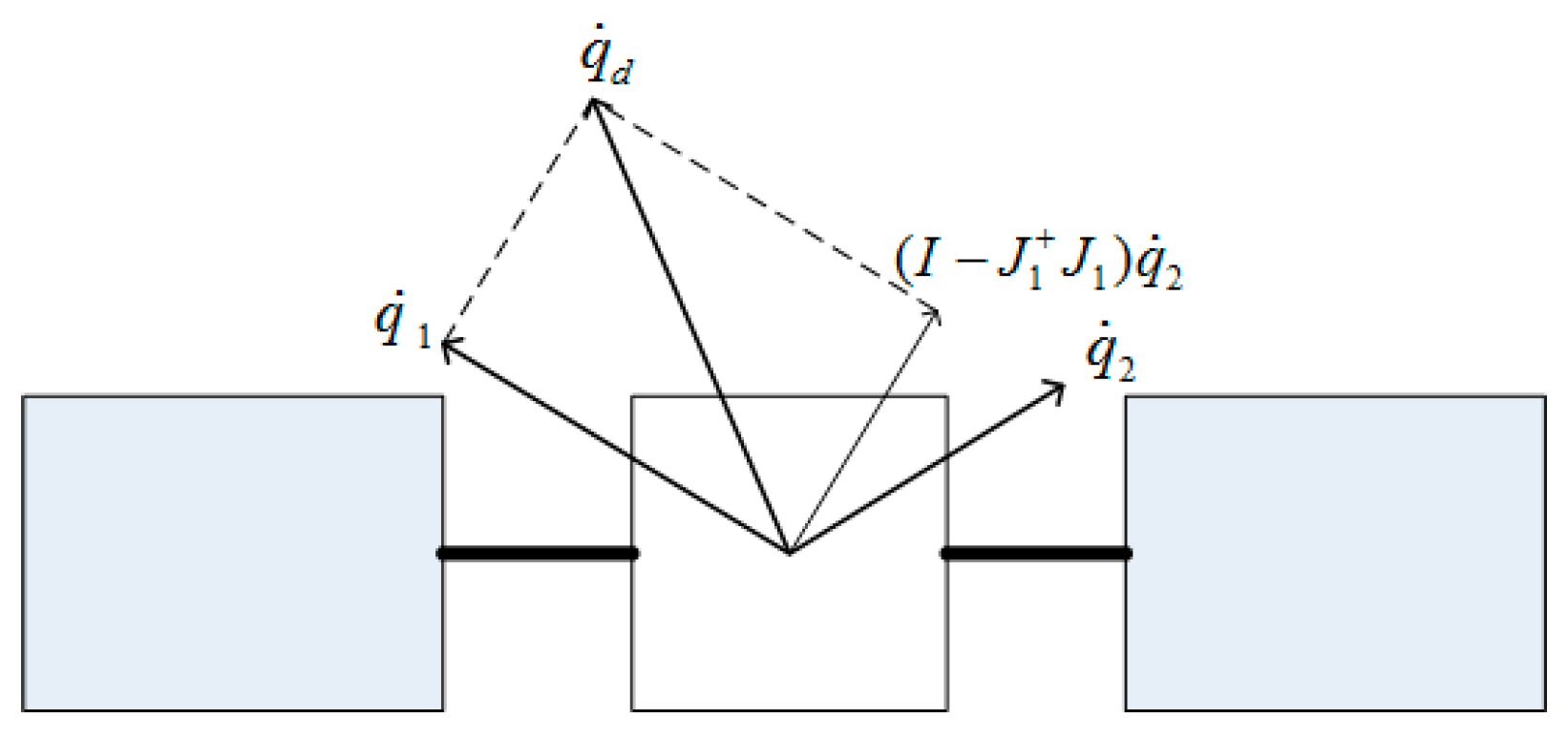
In order to eliminate the conflicting components, the different task velocities need to project onto the null space created by the Jacobian matrices of higher prioritized tasks in NSB control architecture. As shown in Figure 3, ${\dot{q}}_2$ needs to be projected onto the null space of ${\dot{q}}_1$. This means that the effective element of each task is combined to construct the integrated velocity command to drive the robot [34].

3.2. Obstacle Avoidance Mission

The obstacle avoidance mission maintains a specified distance between a robot and an obstacle. Each robot is surrounded by a virtual sphere $B_{i,o}=\left\{q_i,q_i^o\in {ℝ}^p:\Vert q_i-q_i^o\Vert \le d_i\right\}$, where $q_i^o$ indicates the position of the current obstacle for the $i$ th robot, and $B_{i,o}$ indicates the sphere ${\sigma }_{i,1d}=d_i$, where $d_i$ is the minimum allowed safe distance between the $i$ th robot and an obstacle [33].

The obstacle avoidance task function and the error of the task function are represented as

$${\sigma }_{i,1}=\max \left\{\Vert q_i-q_i^o\Vert ,d_i\right\}$$

$${\tilde{\sigma }}_{i,1}={\sigma }_{i,1d}-{\sigma }_{i,1}$$

(3)

Furthermore, we denote $J_1=\left[J_{1,1},\dots J_{n,1}\right]\in {ℝ}^{1\times pn}$, ${\dot{q}}_{i,1}=J_{i,1}^{†}{\lambda }_{i,1}{\tilde{\sigma }}_{i,1}={\lambda }_{i,1}\left(\max \left\{d_i-\Vert q_i-q_i^o\Vert ,0\right\}\right){\widehat{r}}_i$, where $J_{i,1}={\widehat{r}}_i^T$ is the Jacobian matrix, a unity vector pointing at the nearest obstacle is ${\widehat{r}}_i=\left(q_i-q_i^o\right)/\Vert q_i-q_i^o\Vert$, ${\lambda }_{i,1}>0$ is a state-dependent gain to be defined in the next section, and $J_{i,1}^{†}=J_{i,1}^T$. Note that ${\tilde{\sigma }}_{i,1}={\sigma }_{i,1d}-{\sigma }_{i,1}\ge 0$ only if the robot is close enough to the obstacle, and ${\tilde{\sigma }}_{i,1}=0$ when the mission is inactive. This task is built individually for each robot and not as an aggregate task function.

3.3. Escort Mission

In an escort mission, all of the robots scatter around the target evenly. The movements are not known a priori but can be measured in real time. The robots escort the target at a fixed distance in the $p-$ dimensional case (where $p\ge 2$ is a positive integer). Two tasks must be defined: A task for evenly scattering the robots around the target, and a task for maintaining the platoon on the surface of a sphere/hypersphere.

3.3.1. Task for Scattering Robots Around the Target Evenly

With reference to the planar case, the requirement of evenly scattering the robots around the target is satisfied by letting $n$ robots stay at the vertices of a regular polygon of order $n$, in which the distances between adjacent vertices are equal.

In the planar case, a vector $k$ is defined as the index that identifies the robots in their order along the circle. Thus, $k_j$ is the index that identifies the robot at the $j$ th place along the circle, which is not necessarily the $j$ th robot, and $k_j$ and $k_{j+1}$ are indexes that identify two consecutive robots along the circle. Obviously, any robot can be chosen as $k_1$, and $k_1$ and $k_n$ are consecutive indexes [17].

This task function, the desired task function, and the error of the task function are defined as

$${\sigma }_2={\left[\frac{1}{2}{\left(p_{k_1}-p_{k_n}\right)}^T\left(p_{k_1}-p_{k_n}\right),\dots \frac{1}{2}{\left(p_{k_j}-p_{k_{j-1}}\right)}^T\left(p_{k_j}-p_{k_{j-1}}\right),\dots \right]}^T$$

$${\sigma }_{2d}={\left[\frac{l_i{}^2}{2},\dots \frac{l_i{}^2}{2}\right]}^T$$

$${\tilde{\sigma }}_2={\sigma }_{2d}-{\sigma }_2$$

(4)

where $l_i$ is the proper distance between two neighboring robots.

The desired velocity of this task is ${\dot{q}}_2=J_2^{†}{\mathsf{\Lambda }}_2{\tilde{\sigma }}_2$. The corresponding Jacobian matrix is $J_2=block\begin{array}{c}\end{array}diag\left\{{\left(p_{k_1}-p_{k_n}\right)}^T,\dots {\left(p_{k_j}-p_{k_{j-1}}\right)}^T,\dots \right\}\in {ℝ}^{n\times pn}$, whose pseudoinverse is $J_2^{†}=block\begin{array}{c}\end{array}diag\left\{\frac{\left(p_{k_1}-p_{k_n}\right)}{{\left(p_{k_1}-p_{k_n}\right)}^T\left(p_{k_1}-p_{k_n}\right)},\dots \frac{{\left(p_{k_j}-p_{k_{j-1}}\right)}^{}}{{\left(p_{k_j}-p_{k_{j-1}}\right)}^T\left(p_{k_j}-p_{k_{j-1}}\right)},\dots \right\}\in {ℝ}^{pn\times n}$. ${\mathsf{\Lambda }}_2\in {ℝ}^{n\times n}$ represents a constant positive definite matrix of gains.

3.3.2. Task for Maintaining a Platoon on the Surface of a Sphere/Hypersphere

This task function, the desired task function, and the error of the task function are

$${\sigma }_3={\left[\frac{1}{2}{\left(q_1-c\right)}^T\left(q_1-c\right),\dots \frac{1}{2}{\left(q_n-c\right)}^T\left(q_n-c\right)\right]}^T$$

$${\sigma }_{3d}={\left[\frac{R^2}{2},\dots \frac{R^2}{2}\right]}^T$$

$${\tilde{\sigma }}_3={\sigma }_{3d}-{\sigma }_3$$

(5)

${\dot{q}}_3$ is the desired velocity vector for maintaining the robots on the surface of a sphere/hypersphere at a given distance $R$ from the target $c$. ${\dot{q}}_3=J_3^{†}{\mathsf{\Lambda }}_3{\tilde{\sigma }}_3$, where the corresponding Jacobian matrix is $J_3=block\begin{array}{c}\end{array}diag\left\{{\left(q_1-c\right)}^T,\dots {\left(q_n-c\right)}^T\right\}\in {ℝ}^{n\times pn}$ and its pseudoinverse is $J_3^{†}=block\begin{array}{c}\end{array}diag\left\{\frac{\left(q_1-c\right)}{{\left(q_1-c\right)}^T\left(q_1-c\right)},\dots \frac{{\left(q_n-c\right)}^{}}{{\left(q_n-c\right)}^T\left(q_n-c\right)}\right\}\in {ℝ}^{pn\times n}$, and ${\mathsf{\Lambda }}_3\in {ℝ}^{n\times n}$ which is defined similar to ${\mathsf{\Lambda }}_2$ is also a constant positive definite matrix of gains [33].

Remark 1.

In the planar case, robots are distributed at the vertices of a regular polygon, and $l_i$ can be designated as $2R\cos \left(\frac{\pi }{2}-\frac{\pi }{n}\right)$ [17]. However, in three-dimensional and $p-$ dimensional space $\left(p>3\right)$, the problem of how to distribute points on the sphere/hypersphere is treated as a Thomson problem [35,36]. Many scholars have studied this problem and the proper distance does indeed exist.

Remark 2.

If a robot goes out of control and enters another robot’s virtual sphere ${{\rm B}}_{i,o}$, it will be considered as an obstacle, and the rest of the robots must avoid it. If two or more obstacles are considered at the same time, the closest one will be dealt with first [33].

4. Inner Loop Controller Design

The inner loop control is a combination of linear PD control and nonlinear SMC with adaptive control. The PD control part is used to stabilize the nominal model, the SMC part is used to compensate the external disturbances and system uncertainties, and the adaptive control part is utilized to estimate the unknown system parameters.

4.1. APD-SMC Law

The control problem involves designing controllers such that each robot tracks the desired trajectory $q_d\left(t\right)={[q_{1,d}^T(t),\dots q_{n,d}^T(t)]}^T\in {ℝ}^{pn}$, which can be calculated by integrating ${\dot{q}}_d\left(t\right)$ in Equation (2). ${\ddot{q}}_d\left(t\right)$ is defined similarly, and they are all bounded functions. $e={\left[e_1^T,\dots e_n^T\right]}^T=q_d(t)-q(t)\in {ℝ}^{pn}$ and $\dot{e}={\left[{\dot{e}}_1^T,\dots {\dot{e}}_n^T\right]}^T={\dot{q}}_d(t)-\dot{q}(t)\in {ℝ}^{pn}$ are the tracking error and tracking velocity error, respectively.

The nominal reference states ${\dot{q}}_r$ are defined as

$${\dot{q}}_r={\dot{q}}_d+\gamma e$$

$${\ddot{q}}_r={\ddot{q}}_d+\gamma \dot{e}$$

(6)

where ${\dot{q}}_r={\left[{\dot{q}}_{1,r}^T,\dots {\dot{q}}_{n,r}^T\right]}^T$, and $\gamma =diag\left({\gamma }_1,{\gamma }_2\dots {\gamma }_n\right)$ which is positive diagonal matrix, is defined as the sliding constant. Then, the sliding surface is

$$s={\dot{q}}_r-\dot{q}={\dot{q}}_d-\dot{q}+\gamma e=\dot{e}+\gamma e$$

(7)

where $s={\left[s_1^T,\dots s_n^T\right]}^T$. Based on Property 3, the following reference torque is described as follows:

$${\rho }_i=M_i({\mathrm{q}}_i){\ddot{\mathrm{q}}}_{i,r}+C_i(q_i,{\dot{q}}_i){\dot{q}}_{i,r}+g_i\left(q_i\right)=Y_i(q_i,{\dot{q}}_i,{\dot{q}}_{i,r},{\ddot{q}}_{i,r}){\mathsf{\Theta }}_i$$

(8)

For the coordinated control of multiple Euler–Lagrange systems, the APD-SMC law is proposed as

$${\tau }_i={\widehat{\rho }}_i+k_{pi}{e}_i+k_{di}{\dot{e}}_i+k_{i}sign(s_i)$$

(9)

where $k_{pi}$ and $k_{di}$ are the proportional and derivative gains of the PD control, respectively, and $k_i$ is the gain of the robust term. All three gain matrices are selected to be positive definite. ${\widehat{\rho }}_i$ is the estimation of the reference torque ${\rho }_i$ that will be updated using an adaptive law. Owing to the use of APD-SMC, the need for large control gains of PD-SMC to compensate for the unknown term ${\rho }_i$ is avoided.

$${\dot{\widehat{\rho }}}_i={\mu }_i{s}_i$$

$${\widehat{\rho }}_i(0)={\widehat{\rho }}_{i,0}$$

(10)

where ${\mu }_i$ represents the diagonal matrix adaptation rate and ${\widehat{\rho }}_{i,0}$ is the initial value of the estimated torque vector.

Remark 3.

It can be seen that the APD-SMC law in Equation (9) is only related to the tracking error $e_i$ and tracking velocity error ${\dot{e}}_i$. Therefore, the control law is model-free and easy to implement in practice.

4.2. Stability Analysis

From Equation (7), we have

$${\dot{s}}_i={\ddot{e}}_i+{\gamma }_i{\dot{e}}_i$$

$${\ddot{q}}_i={\ddot{q}}_{i,r}-{\dot{s}}_i$$

(11)

According to Equations (1), (8) and (11), the following equation can be obtained:

$$M_i(q_i){\dot{s}}_i+C_i\left(q_i,{\dot{q}}_i\right)s_i+{\tau }_i={\rho }_i-{\tau }_i^d,i=1,\dots ,n$$

(12)

Theorem 1.

Consider the errors of task functions in Equations (3)–(5), the Euler–Lagrange system in Equation (1) with the proposed APD-SMC law in Equation (9), and adaptation update law in Equation (10). Suppose that Properties 1–4 hold. We can conclude that

• If there is no conflict between the three tasks, then they can be fulfilled simultaneously. The system is globally asymptotically stable, and the tracking error $e_i$ can converge to zero.
• If an obstacle avoidance mission is active and conflicts with an escort mission, then the gain is chosen as ${\lambda }_{i,1}\left(\Vert e_i\Vert ,\Vert {\dot{q}}_i\Vert \right)={\lambda }_{i,1}^{★}\left(\Vert e_i\Vert ,\Vert {\dot{q}}_i\Vert \right)+{\varrho }_i$, where ${\varrho }_i$ is designed based on robustness to noise, for example, measurement noise. Then, the obstacle avoidance mission is fulfilled first. Furthermore, the system is globally asymptotically stable, and the tracking error $e_i$ can converge to zero.

Proof. 

The overall Lyapunov function candidate $V$ is considered as

$$V=V_1+V_2$$

$$V_1=\frac{1}{2}\left({\displaystyle \sum _{i=1}^n{s}_i{}^T{M}_i{s}_i}+{\displaystyle \sum _{i=1}^n{e}_i{}^T(k_{p_i}+{\gamma }_i{k}_{di})e_i}+{\displaystyle \sum _{i=1}^n\frac{1}{{\mu }_i}{\tilde{\rho }}_i^T{\tilde{\rho }}_i}\right)$$

$$V_2=\frac{1}{2}\left({\tilde{\sigma }}_1^T{\eta }_1{\tilde{\sigma }}_1+{\tilde{\sigma }}_2^T{\eta }_2{\tilde{\sigma }}_2+{\tilde{\sigma }}_3^T{\eta }_3{\tilde{\sigma }}_3\right)$$

(13)

where ${\tilde{\rho }}_i={\rho }_i-{\widehat{\rho }}_i$. ${\eta }_1$, ${\eta }_2$, and ${\eta }_3$ are design parameters, and ${\tilde{\sigma }}_1={\displaystyle \sum _{i=1}^n{\tilde{\sigma }}_{i,1}}$. The inertia matrix $M_i$ is positive definite. $k_{pi}$, $k_{di}$, ${\eta }_1$, ${\eta }_2$, and ${\eta }_3$ are selected as positive definite. It can be easily proven that $V$ is a positive definite function. Based on Equations (9) and (12), the following equation can be obtained:

$$M_i(q_i){\dot{s}}_i={\rho }_i-C_i(q_{i,}{\dot{q}}_i)s_i-{\tau }_i^d-{\widehat{\rho }}_i-k_{pi}{e}_i-k_{di}{\dot{e}}_i-k_{i}sign(s_i)$$

(14)

Differentiating $V_1$ with respect to time yields

$${\dot{V}}_1={\displaystyle \sum _{i=1}^n{s}_i^T{M}_i\left(q_i\right){\dot{s}}_i}+{\displaystyle \sum _{i=1}^n\frac{1}{2}}{s}_i^T{\dot{M}}_i\left(q_i\right)s_i+{\displaystyle \sum _{i=1}^n{e}_i^T(k_{pi}+{\gamma }_i{k}_{di}){\dot{e}}_i}-{\displaystyle \sum _{i=1}^n\frac{1}{{\mu }_i}}{\tilde{\rho }}_i^T{\dot{\widehat{\rho }}}_i$$

(15)

Applying Equations (7), (10), and (14) to Equation (15), we have

$$\begin{array}{l}{\dot{V}}_1={\displaystyle \sum _{i=1}^n{\tilde{\rho }}_i^T{s}_i-{\displaystyle \sum _{i=1}^n\frac{1}{{\mu }_i}}}{\tilde{\rho }}_i^T{\dot{\widehat{\rho }}}_i+{\displaystyle \sum _{i=1}^n{s}_i^T\left(\frac{1}{2}{\dot{M}}_i(q_i)-C_i(q_{i,}{\dot{q}}_i)\right)}{s}_i-{\displaystyle \sum _{i=1}^n{s}_i^T{k}_{i}sign(s_i)}\\ -{\displaystyle \sum _{i=1}^n({\dot{e}}_i^T+{\gamma }_i{e}_i^T)(k_{pi}{e}_i+k_{di}{\dot{e}}_i)+}{\displaystyle \sum _{i=1}^n{e}_i^T(k_{pi}+{\gamma }_i{k}_{di}){\dot{e}}_i}-{\displaystyle \sum _{i=1}^n{s}_i^T{\tau }_i^d}\\ ={\displaystyle \sum _{i=1}^n{\tilde{\rho }}_i^T{s}_i-{\displaystyle \sum _{i=1}^n\frac{1}{{\mu }_i}}}{\tilde{\rho }}_i^T{\dot{\widehat{\rho }}}_i+{\displaystyle \sum _{i=1}^n{s}_i^T\left(\frac{1}{2}{\dot{M}}_i(q_i)-C_i(q_{i,}{\dot{q}}_i)\right)}{s}_i-{\displaystyle \sum _{i=1}^n{s}_i^T{k}_{i}sign(s_i)}\\ -{\displaystyle \sum _{i=1}^n{\gamma }_i{e}_i^T{k}_{p_i}{e}_i}-{\displaystyle \sum _{i=1}^n{\dot{e}}_i^T{k}_{di}{\dot{e}}_i}-{\displaystyle \sum _{i=1}^n{s}_i^T{\tau }_i^d}\\ =-{\displaystyle \sum _{i=1}^n{s}_i^T{k}_{i}sign(s_i)}-{\displaystyle \sum _{i=1}^n{\gamma }_i{e}_i^T{k}_{pi}{e}_i}-{\displaystyle \sum _{i=1}^n{\dot{e}}_i^T{k}_{di}{\dot{e}}_i}-{\displaystyle \sum _{i=1}^n{s}_i^T{\tau }_i^d}\le 0\end{array}$$

(16)

The Lyapunov function $V_1$ is positive definite, and its time derivative ${\dot{V}}_1$ is negative definite. It is concluded that the inner loop subsystem is globally asymptotically stable, and the tracking error $e_i$ could converge to zero with APD-SMC according to the Lyapunov method. In the above equation, the equality ${\dot{V}}_1=0$ is satisfied only if $e_i={\dot{e}}_i=0$. □

Remark 4.

In practice, the discontinuous term $sign(\cdot )$ function in Equation (9) may cause chattering problems. To avoid the chattering problems, a saturation function $tanh(\cdot )$ is introduced to replace the discontinuous $sign(\cdot )$ function [31].

Then, the control law in Equation (9) is modified to

$${\tau }_i={\widehat{\rho }}_i+k_{pi}{e}_i+k_{di}{\dot{e}}_i+k_{i}tanh(s_i)$$

(17)

where $tanh(s_i)=\frac{e_i^{s_i}-e_i^{-s_i}}{e_i^{s_i}+e_i^{-s_i}}$.

Using Equation (13), we obtain

$$\begin{array}{l}{\dot{V}}_2=-{\eta }_1{\tilde{\sigma }}_1^T{\dot{\sigma }}_1-{\eta }_2{\tilde{\sigma }}_2^T{\dot{\sigma }}_2-{\tilde{\sigma }}_3^T{\eta }_3{\dot{\sigma }}_3\\ =-{\tilde{\sigma }}_1^T{\eta }_1{J}_1{\dot{q}}_d-{\tilde{\sigma }}_2^T{\eta }_2{J}_2{\dot{q}}_d-{\tilde{\sigma }}_3^T{\eta }_3{J}_3{\dot{q}}_d\\ =-{\eta }_1{\tilde{\sigma }}_1^T\left(J_1{J}_1^{+}{\lambda }_1{\tilde{\sigma }}_1+J_1(I-J_1^{+}{J}_1)(J_2^{+}{\mathsf{\Lambda }}_2{\tilde{\sigma }}_2+(I-J_2^{+}{J}_2)J_3^{+}{\mathsf{\Lambda }}_3{\tilde{\sigma }}_3)\right)\\ -{\eta }_2{\tilde{\sigma }}_2^T\left(J_2{J}_1^{+}{\lambda }_1{\tilde{\sigma }}_1+J_2(I-J_1^{+}{J}_1)(J_2^{+}{\mathsf{\Lambda }}_2{\tilde{\sigma }}_2+(I-J_2^{+}{J}_2)J_3^{+}{\mathsf{\Lambda }}_3{\tilde{\sigma }}_3)\right)\\ -{\eta }_3{\tilde{\sigma }}_3^T\left(J_3{J}_1^{+}{\lambda }_1{\tilde{\sigma }}_1+J_3(I-J_1^{+}{J}_1)(J_2^{+}{\mathsf{\Lambda }}_2{\tilde{\sigma }}_{12}+(I-J_2^{+}{J}_2)J_3^{+}{\mathsf{\Lambda }}_3{\tilde{\sigma }}_3)\right)\\ =-{\tilde{\sigma }}_1^T{\eta }_1{\lambda }_1{\tilde{\sigma }}_1-{\tilde{\sigma }}_2^T{\eta }_2{\mathsf{\Lambda }}_2{\tilde{\sigma }}_2-{\tilde{\sigma }}_3^T{\eta }_3{\mathsf{\Lambda }}_3{\tilde{\sigma }}_3-{\tilde{\sigma }}_2^T{\eta }_2{\lambda }_1{J}_2{J}_1^{+}{\tilde{\sigma }}_1-{\tilde{\sigma }}_3^T{\eta }_3{\lambda }_1{J}_3{J}_1^{+}{\tilde{\sigma }}_1\\ -{\tilde{\sigma }}_3^T{\eta }_3{\mathsf{\Lambda }}_2{J}_3{J}_2^{+}{\tilde{\sigma }}_2+{\tilde{\sigma }}_2^T{\eta }_2{\mathsf{\Lambda }}_2{J}_2{J}_1^{+}{J}_1{J}_2^{+}{\tilde{\sigma }}_2+{\tilde{\sigma }}_2^T{\eta }_2{J}_2{J}_1^{+}{J}_1{J}_3^{+}{\mathsf{\Lambda }}_3{\tilde{\sigma }}_3+{\tilde{\sigma }}_3^T{\eta }_3{J}_3{J}_2^{+}{J}_2{J}_3^{+}{\mathsf{\Lambda }}_3{\tilde{\sigma }}_3\\ +{\tilde{\sigma }}_3^T{\eta }_3{\mathsf{\Lambda }}_2{J}_3{J}_1^{+}{J}_1{J}_2^{+}{\tilde{\sigma }}_2+{\tilde{\sigma }}_3^T{\eta }_3{J}_3{J}_1^{+}{J}_1{J}_3^{+}{\mathsf{\Lambda }}_3{\tilde{\sigma }}_3-{\tilde{\sigma }}_2^T{\eta }_2{J}_2{J}_1^{+}{J}_1{J}_2^{+}{J}_2{J}_3^{+}{\mathsf{\Lambda }}_3{\tilde{\sigma }}_3-{\tilde{\sigma }}_3^T{\eta }_3{J}_3{J}_1^{+}{J}_1{J}_2^{+}{J}_2{J}_3^{+}{\mathsf{\Lambda }}_3{\tilde{\sigma }}_3\end{array}$$

(18)

Next, two different cases will be discussed separately: Conflicting and nonconflicting tasks. Assuming there is no conflict between each pair of tasks, an interesting property of the Jacobian matrices is utilized so that the nonconflicting relationship between three tasks can be expressed as

$$J_2{J}_1^{+}=0$$

$$J_3{J}_1^{+}=0$$

$$J_3{J}_2^{+}=0$$

(19)

It means that the three tasks projected onto the robot velocity space are orthogonal. Therefore, they may be fulfilled simultaneously [37]. Inserting Equation (19) into Equation (18), we obtain

$${\dot{V}}_2=-{\tilde{\sigma }}_1^T{\eta }_1{\lambda }_1{\tilde{\sigma }}_1-{\tilde{\sigma }}_2^T{\eta }_2{\mathsf{\Lambda }}_2{\tilde{\sigma }}_2-{\tilde{\sigma }}_3^T{\eta }_3{\mathsf{\Lambda }}_3{\tilde{\sigma }}_3\le 0$$

(20)

Accordingly, from the above analysis, we find that if there is no conflict between every pair of tasks, then the outer loop subsystem is globally asymptotically stable. Meanwhile, if the obstacle avoidance mission is active and conflicts with the escort mission, then ${\dot{V}}_2$ is in the form

$${\dot{V}}_2=-X^{T}PX$$

(21)

where $X={\left[{\tilde{\sigma }}_1^T,{\tilde{\sigma }}_2^T,{\tilde{\sigma }}_3^T\right]}^T$ and $P=\left[p_{ij}\right],i,j=1,2,3$ with submatrices given by $p_{11}={\eta }_1{\lambda }_1$, $p_{21}={\eta }_2{\lambda }_1{J}_2{J}_1^{+}$, $p_{22}={\eta }_2{\mathsf{\Lambda }}_2-{\eta }_2{\mathsf{\Lambda }}_2{J}_2{J}_1^{+}{J}_1{J}_2^{+}$, $p_{23}=-{\eta }_2{J}_2{J}_1^{+}{J}_1{J}_3^{+}{\mathsf{\Lambda }}_3+{\eta }_2{J}_2{J}_1^{+}{J}_1{J}_2^{+}{J}_2{J}_3^{+}{\mathsf{\Lambda }}_3$, $p_{31}={\eta }_3{\lambda }_1{J}_3{J}_1^{+}$, $p_{32}={\eta }_3{\mathsf{\Lambda }}_2{J}_3{J}_2^{+}-{\eta }_3{\mathsf{\Lambda }}_2{J}_3{J}_1^{+}{J}_1{J}_2^{+}$, and $p_{33}={\eta }_3{\mathsf{\Lambda }}_3-{\eta }_3{J}_3{J}_2^{+}{J}_2{J}_3^{+}{\mathsf{\Lambda }}_3-{\eta }_3{J}_3{J}_1^{+}{J}_1{J}_3^{+}{\mathsf{\Lambda }}_3+{\eta }_3{J}_3{J}_1^{+}{J}_1{J}_2^{+}{J}_2{J}_3^{+}{\mathsf{\Lambda }}_3$. We apply $2\left|ab\right|\le a^2+b^2$ for any $a,b\in ℝ$ to obtain

$$\begin{array}{l}{X}^{T}PX\ge \left(p_{11,m}-p_{12,M}-p_{13,M}\right){\Vert {\tilde{\sigma }}_1\Vert }^2\\ +\left(p_{22,m}-p_{21,M}-p_{22,M}\right){\Vert {\tilde{\sigma }}_2\Vert }^2\\ +\left(p_{33,m}-p_{31,M}-p_{32,M}\right){\Vert {\tilde{\sigma }}_3\Vert }^2\end{array}$$

(22)

where $p_{ij,m}$ and $p_{ij,M}$ denote the lower and upper bounds, respectively, on the induced norms of subblocks $p_{ij}$ of $P$.

$X^{T}PX\ge \frac{1}{2}\left(p_{11,m}{\Vert {\tilde{\sigma }}_1\Vert }^2+p_{22,m}{\Vert {\tilde{\sigma }}_2\Vert }^2+p_{33,m}{\Vert {\tilde{\sigma }}_3\Vert }^2\right)$. We see that since $\Vert J_1\Vert =\Vert J_2\Vert =\Vert J_3\Vert =1$, $p_{22,m}=p_{22,M}=0$, and $p_{33,m}=p_{33,M}=0$, we lose control of ${\tilde{\sigma }}_2$ and ${\tilde{\sigma }}_3$. $V_2$ should be reselected as $V_2=\frac{1}{2}{\tilde{\sigma }}_1^T{\eta }_1{\tilde{\sigma }}_1$ in this situation. Then, we obtain ${\dot{V}}_2=-{\tilde{\sigma }}_1^T{\eta }_1{\lambda }_1{\tilde{\sigma }}_1\le 0$. Similarly, the outer loop subsystem is globally asymptotically stable.

In this situation, the solution in Theorem 1, which implies that obstacle avoidance mission has a higher priority and will be fulfilled first when it conflicts with the escort mission, is achieved. Then, the escort mission can be accomplished when there is no conflict. As the NSB method is kinematic, acting on the dynamics through the desired velocity and not the desired position, it is necessary to design ${\lambda }_{i,1}$ properly to make the velocity error dominate the position error.

The sliding surface (7) contains both position and velocity errors. By inserting Equation (2) into Equation (7) and considering the fact that if every two tasks conflict, then the contributions from ${\tilde{\sigma }}_2$ and ${\tilde{\sigma }}_3$ can be removed, thus ${\dot{q}}_d={\dot{q}}_1$. We require that

$$\begin{array}{l}{\left({\dot{q}}_i-J_{i,1}^{+}{\lambda }_{i,1}{\tilde{\sigma }}_{i,1}\right)}^T{k}_{di}\left({\dot{q}}_i-J_{i,1}^{+}{\lambda }_{i,1}{\tilde{\sigma }}_{i,1}\right)\\ >k_{di}{e}_i^T{\gamma }_i{}^2{e}_i+k_{di}{\gamma }_i{e}_i{\left({\dot{q}}_i-J_{i,1}^{+}{\lambda }_{i,1}{\tilde{\sigma }}_{i,1}\right)}^T+k_{di}{\gamma }_i{e}_i^T\left({\dot{q}}_i-J_{i,1}^{+}{\lambda }_{i,1}{\tilde{\sigma }}_{i,1}\right)\end{array}$$

(23)

By manipulating Equation (23) as an equality and taking the norm on both sides of it, we obtain

$${\lambda }_{i,1}^{★}\left(\Vert e_i\Vert ,\Vert {\dot{q}}_i\Vert \right)=\frac{b_i+\sqrt{b_i^2+4a_i{c}_i}}{2a_i}$$

$$a_i={\tilde{\sigma }}_{i,1}^2$$

$$b_i=2{\tilde{\sigma }}_{i,1}\left(\Vert {\dot{q}}_i\Vert -2{\gamma }_i\Vert e_i\Vert \right)$$

$$c_i={\gamma }_i^2{\Vert e_i\Vert }^2+2{\gamma }_i\Vert e_i\Vert \Vert {\dot{q}}_i\Vert -{\Vert {\dot{q}}_i\Vert }^2$$

(24)

Thus, by choosing ${\lambda }_{i,1}\left(\Vert e_i\Vert ,\Vert {\dot{q}}_i\Vert \right)={\lambda }_{i,1}^{★}\left(\Vert e_i\Vert ,\Vert {\dot{q}}_i\Vert \right)+{\varrho }_i$, where ${\varrho }_i>0$ is chosen based on the robustness to noise, this constant ensures that the robot moves away from the obstacle.

Remark 5.

If just the two tasks of the escort mission are in conflict, then each robot fulfills only the first two higher-level tasks. Conflicts will not occur where ${\dot{q}}_d={\dot{q}}_1+(I-J_1^{+}{J}_1){\dot{q}}_2$.

Remark 6.

Following [17,38], if a robot is going to frontally collide with an obstacle and the projection along the tangential direction is null, the robot will stop. Measurement noise ${\varrho }_i$ can avoid the local minimum which is caused by this situation.

5. Simulations

Simulation experiments were performed to demonstrate the effectiveness of the proposed algorithm with the adaptation law compared with ASMC in two-dimensional and three-dimensional space in three scenarios.

The dynamic equation of each robot is selected as

$$M_i{\ddot{q}}_i+C_i{\dot{q}}_i={\tau }_i+{\tau }_i^d$$

(25)

The definitions of the parameters are similar to Equation (1). The noise is considered to be contained in a compact set $\sigma {\mathbb{B}}^n=\left\{x\in {ℝ}^n:\Vert x\Vert \le \sigma \right\}$, and the measured states are ${\tilde{q}}_i=\tilde{q}+0.02{\mathbb{B}}^n$ and ${\dot{\tilde{q}}}_i=\dot{\tilde{q}}+0.01{\mathbb{B}}^n$. The control forces are assumed to saturate at $\Vert {\tau }_i\Vert \le 10N$. All parameters of controller are adjusted with a trial and error method to achieve the best performance.

Consider five robots in two-dimensional space. The system parameters are assumed to be $M_i=1$ and $C_i=0$, where $i=1,\dots ,5$. The parameters of the proposed controller and adaptation law are $k_{pi}=30$, $k_{di}=50$, $k_i=1$, $\gamma =diag(20,\dots ,20)$, ${\widehat{\rho }}_{i,0}={[0.1,0.1]}^T$, and ${\mu }_i=20$, where $i=1,\dots ,5$. The mission parameters are $R=5$, $d_i=2$, $l_i=2R\cos \left(\frac{\pi }{2}-\frac{\pi }{5}\right)$, ${\mathsf{\Lambda }}_2={\mathsf{\Lambda }}_3=0.8I$, and ${\varrho }_i=0.1$, where $i=1,\dots ,5$. The external disturbance parameters are ${\tau }_i^d=0.5{[\sin (0.5t),\sin (0.7t)]}^T$, where $i=1,\dots ,5$. The initial positions of the five robots are $q_1(0)={[5,10]}^T$, $q_2(0)={[-5,5]}^T$, $q_3(0)={[-5,-5]}^T$, $q_4(0)={[5,-10]}^T$, and $q_5(0)={[5,0]}^T$.

In three-dimensional space, six robots are considered in the simulations. The corresponding parameters and initial positions are set as $l_i=\sqrt{2}R$, ${\widehat{\rho }}_{i,0}={[0.1,0.1,0.1]}^T$, ${\tau }_i^d=0.5{[\sin (0.5t),\sin (0.7t),cos(0.5t)]}^T$, $i=1,\dots ,6$, $q_1(0)={[-10,1,0]}^T$, $q_2(0)={[-1,-10,0.3]}^T$, $q_3(0)={[10,0,1]}^T$, $q_4(0)={[0,0.5,10]}^T$, $q_5(0)={[0,10,0.3]}^T$, and $q_6(0)={[0,0,-10]}^T$. The other parameters are similar to those in the two-dimensional case.

For literature completeness, an ASMC scheme can be designed as ${\tau }_i={\widehat{\rho }}_i+k_{ai}sign(s_i)$ with the adaptive control law (10). The controller parameter of ASMC is given as $k_{ai}=80$.

In three-dimensional space, the six robots reach the vertices of the regular octahedron, while the target is the centroid, as in Figure 4. The edges of the regular octahedron are the distances between the adjacent robots. Thus, the task function and pseudoinverse of the Jacobian matrix can be rewritten as

$$\begin{array}{l}{\sigma }_{21}=[\frac{1}{2}{\left(p_{k_1}-p_{k_2}\right)}^T\left(p_{k_1}-p_{k_2}\right),\frac{1}{2}{\left(p_{k_2}-p_{k_5}\right)}^T\left(p_{k_2}-p_{k_5}\right),\frac{1}{2}{\left(p_{k_3}-p_{k_4}\right)}^T\left(p_{k_3}-p_{k_4}\right)\\ \frac{1}{2}{\left(p_{k_4}-p_{k_1}\right)}^T\left(p_{k_4}-p_{k_1}\right),\frac{1}{2}{\left(p_{k_5}-p_{k_6}\right)}^T\left(p_{k_5}-p_{k_6}\right),\frac{1}{2}{\left(p_{k_6}-p_{k_3}\right)}^T\left(p_{k_6}-p_{k_3}\right)]\end{array}$$

(26)

$$\begin{array}{l}{\sigma }_{22}=[\frac{1}{2}{\left(p_{k_1}-p_{k_3}\right)}^T\left(p_{k_1}-p_{k_3}\right),\frac{1}{2}{\left(p_{k_2}-p_{k_6}\right)}^T\left(p_{k_2}-p_{k_6}\right),\frac{1}{2}{\left(p_{k_3}-p_{k_2}\right)}^T\left(p_{k_3}-p_{k_2}\right)\\ \frac{1}{2}{\left(p_{k_4}-p_{k_5}\right)}^T\left(p_{k_4}-p_{k_5}\right),\frac{1}{2}{\left(p_{k_5}-p_{k_1}\right)}^T\left(p_{k_5}-p_{k_1}\right),\frac{1}{2}{\left(p_{k_6}-p_{k_4}\right)}^T\left(p_{k_6}-p_{k_4}\right)]\end{array}$$

(27)

$$\begin{array}{l}{J}_{21}^{†}=block\begin{array}{c}\end{array}diag\{\frac{\left(p_{k_1}-p_{k_2}\right)}{\frac{1}{2}{\left(p_{k_1}-p_{k_2}\right)}^T\left(p_{k_1}-p_{k_2}\right)},\frac{\left(p_{k_2}-p_{k_5}\right)}{\frac{1}{2}{\left(p_{k_2}-p_{k_5}\right)}^T\left(p_{k_2}-p_{k_5}\right)},\frac{\left(p_{k_3}-p_{k_4}\right)}{\frac{1}{2}{\left(p_{k_3}-p_{k_4}\right)}^T\left(p_{k_3}-p_{k_4}\right)}\\ \frac{\left(p_{k_4}-p_{k_1}\right)}{\frac{1}{2}{\left(p_{k_4}-p_{k_1}\right)}^T\left(p_{k_4}-p_{k_1}\right)},\frac{\left(p_{k_5}-p_{k_6}\right)}{\frac{1}{2}{\left(p_{k_5}-p_{k_6}\right)}^T\left(p_{k_5}-p_{k_6}\right)},\frac{\left(p_{k_6}-p_{k_3}\right)}{\frac{1}{2}{\left(p_{k_6}-p_{k_3}\right)}^T\left(p_{k_6}-p_{k_3}\right)}\}\end{array}$$

(28)

$$\begin{array}{l}{J}_{22}^{†}=block\begin{array}{c}\end{array}diag\{\frac{\left(p_{k_1}-p_{k_3}\right)}{\frac{1}{2}{\left(p_{k_1}-p_{k_3}\right)}^T\left(p_{k_1}-p_{k_3}\right)},\frac{\left(p_{k_2}-p_{k_6}\right)}{\frac{1}{2}{\left(p_{k_2}-p_{k_6}\right)}^T\left(p_{k_2}-p_{k_6}\right)},\frac{\left(p_{k_3}-p_{k_2}\right)}{\frac{1}{2}{\left(p_{k_3}-p_{k_2}\right)}^T\left(p_{k_3}-p_{k_2}\right)}\\ \frac{\left(p_{k_4}-p_{k_5}\right)}{\frac{1}{2}{\left(p_{k_4}-p_{k_5}\right)}^T\left(p_{k_4}-p_{k_5}\right)},\frac{\left(p_{k_5}-p_{k_1}\right)}{\frac{1}{2}{\left(p_{k_5}-p_{k_1}\right)}^T\left(p_{k_5}-p_{k_1}\right)},\frac{\left(p_{k_6}-p_{k_4}\right)}{\frac{1}{2}{\left(p_{k_6}-p_{k_4}\right)}^T\left(p_{k_6}-p_{k_4}\right)}\}\end{array}$$

(29)

Equation (2) can be rewritten as

$${\dot{q}}_d={\dot{q}}_1+\left(I-J_1^{†}{J}_1\right)[{\dot{q}}_{21}+(I-J_{21}^{+}{J}_{21}){\dot{q}}_3+{\dot{q}}_{22}+(I-J_{22}^{+}{J}_{22}){\dot{q}}_3]$$

(30)

All simulation experiments were conducted in MATLAB R2016a on a PC with Intel^® Core I5-4590 and a 3.6-GHz CPU, 12 GB of RAM, and 1000-GB solid-state disk drive.

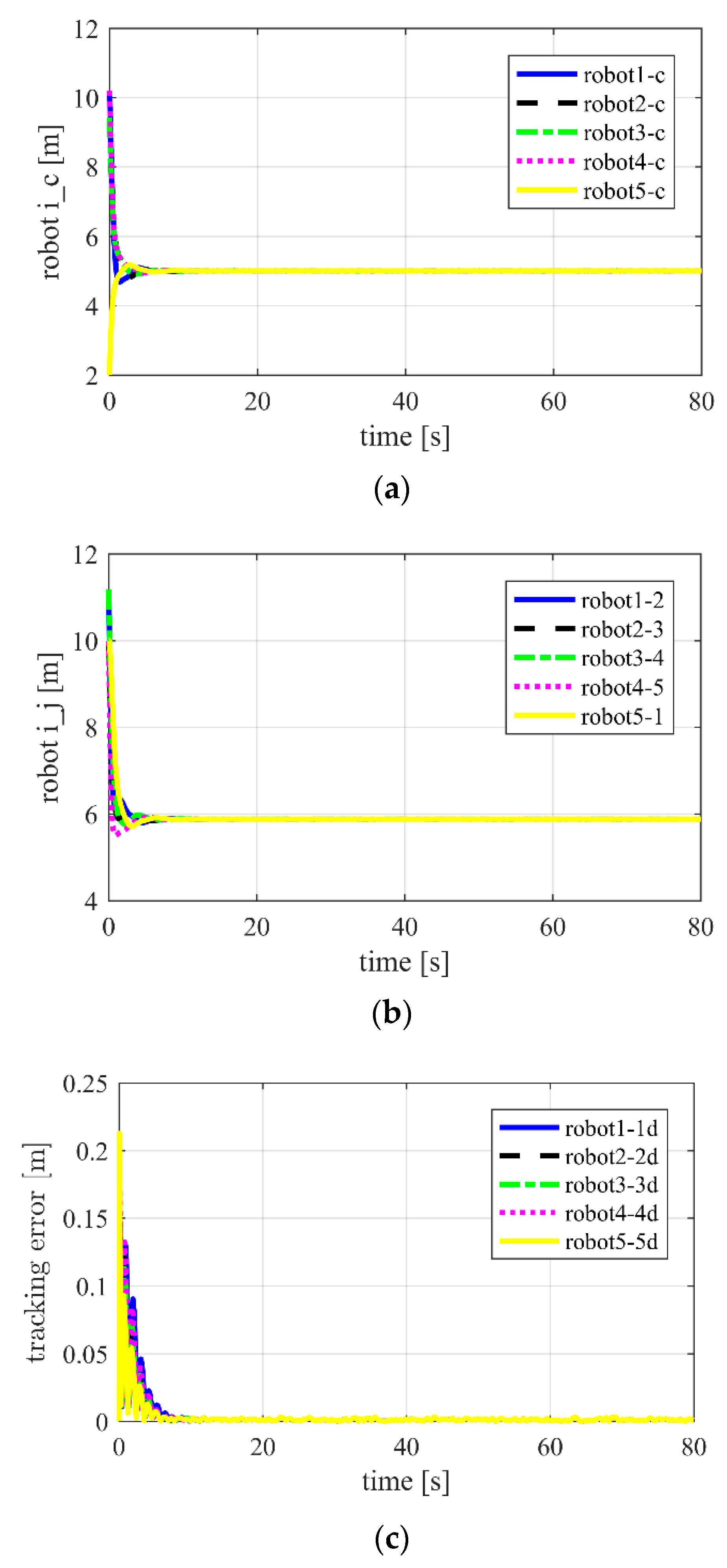
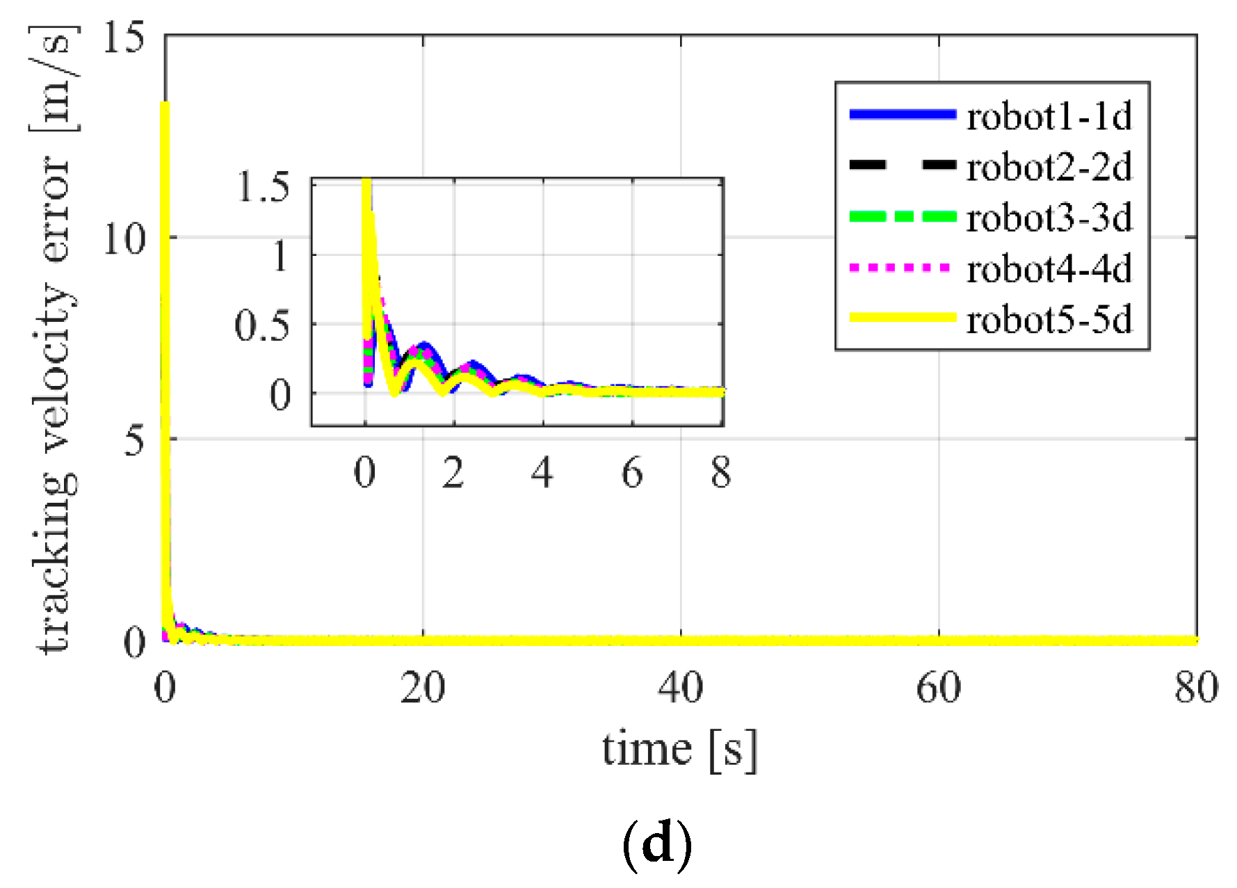
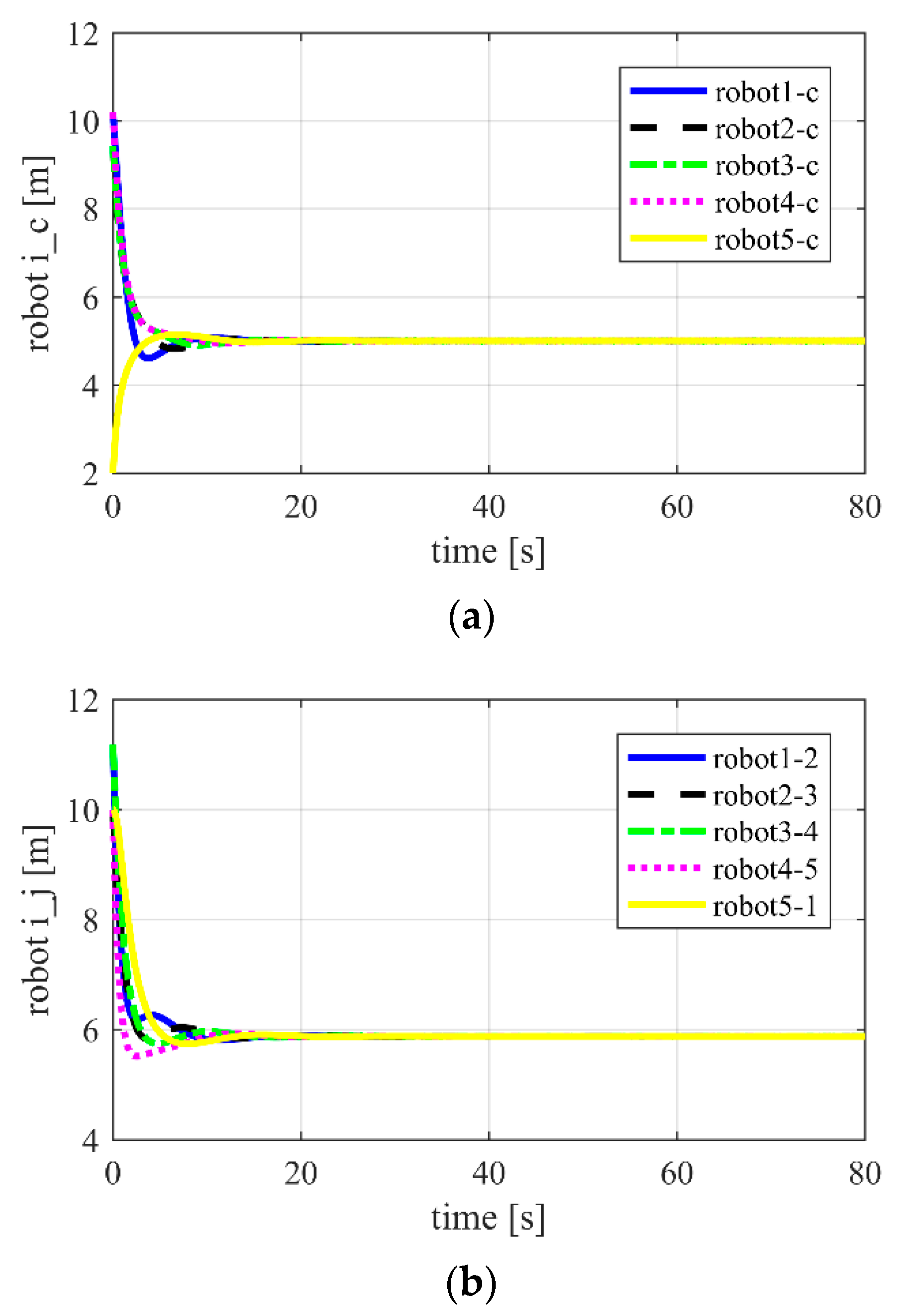
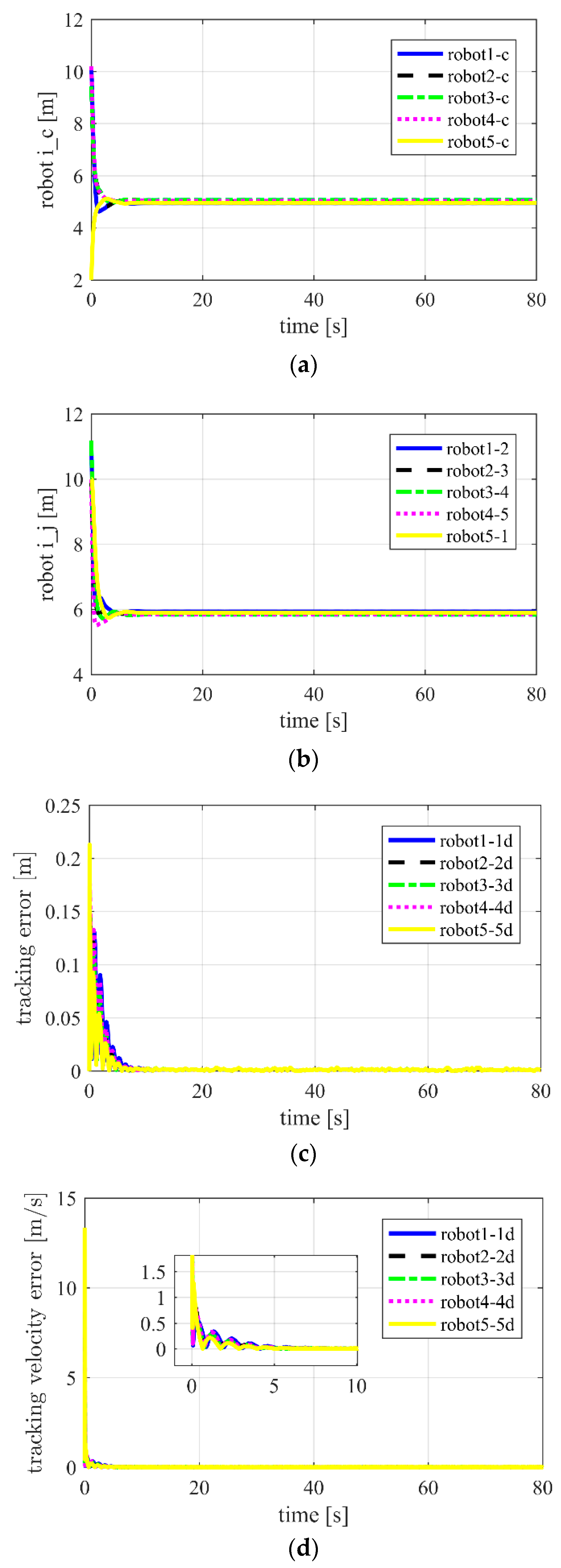
5.1. Case 1: Escorting a Stationary Target

5.1.1. In Two-Dimensional Space

Five robots escort a stationary target $c={[3,0]}^T$ in this scenario. Figure 5 shows the distances between the robot and target, the distances between the neighboring robots, and position tracking errors with APD-SMC.

It is shown that all of the robots can maintain the fixed distance from the target and surround it evenly. Figure 6 shows much worse control performance compared with using APD-SMC. This further verifies that convergence can be achieved faster and with higher control precision than ASMC.

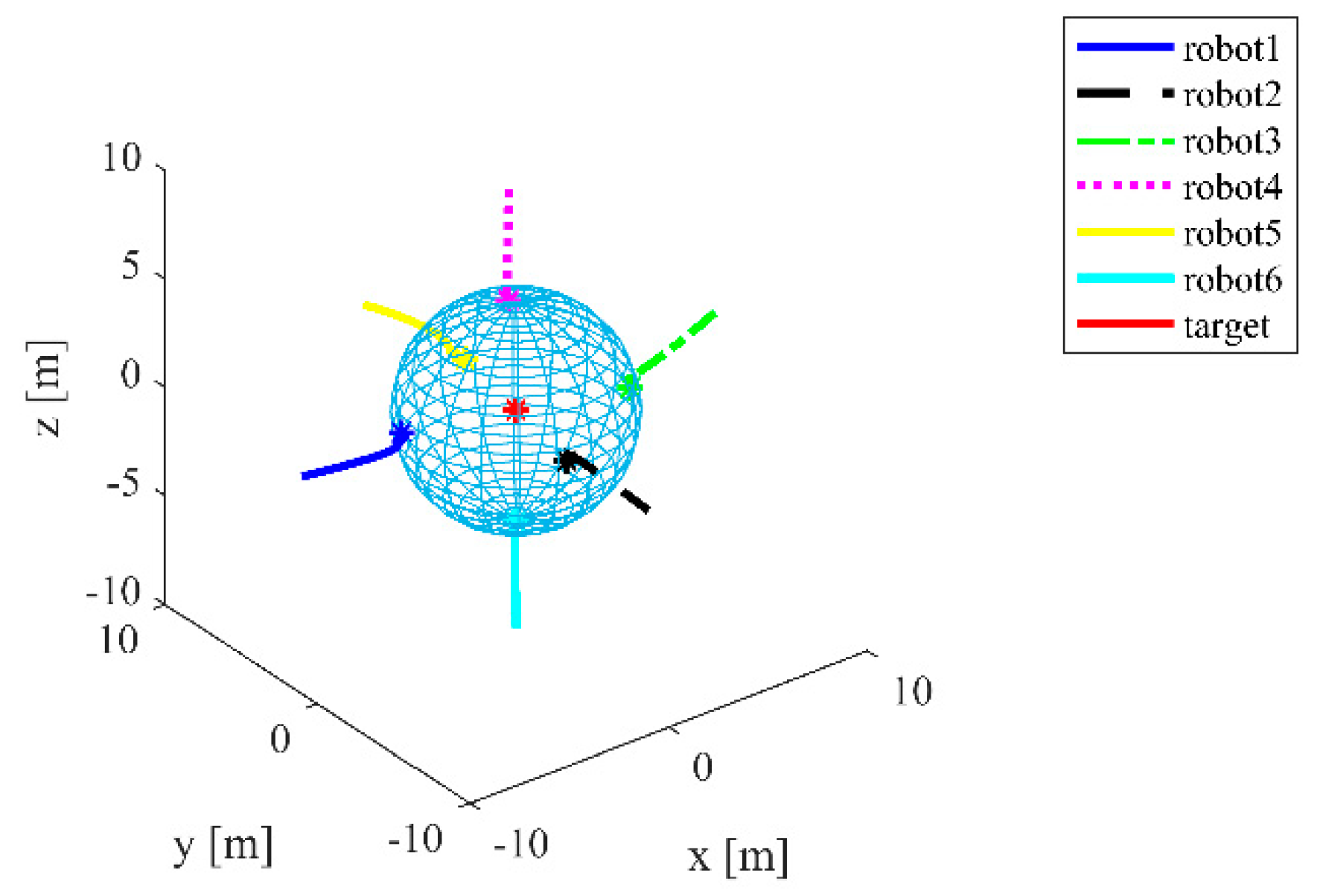
5.1.2. In Three-Dimensional Space

Figure 7 shows the robot trajectories in three-dimensional space with the target $c={[0,0,0]}^T$. This validates the effectiveness of the APD-SMC control algorithm in three-dimensional space.

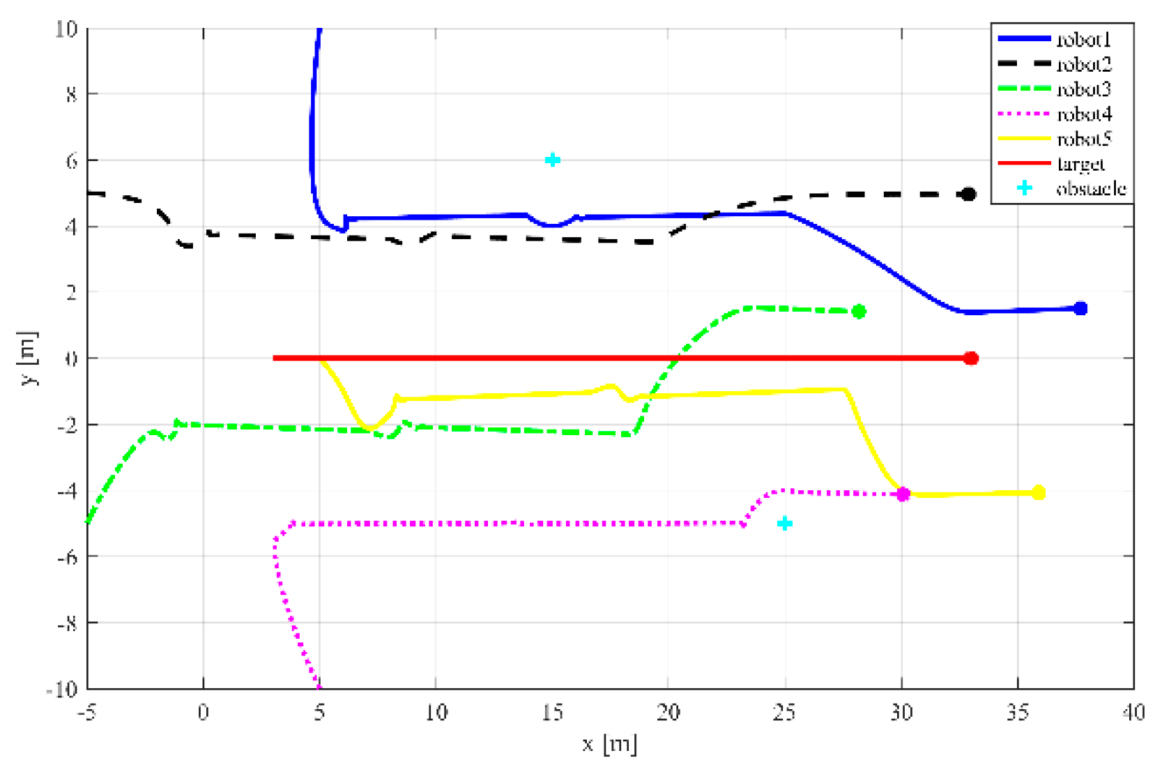
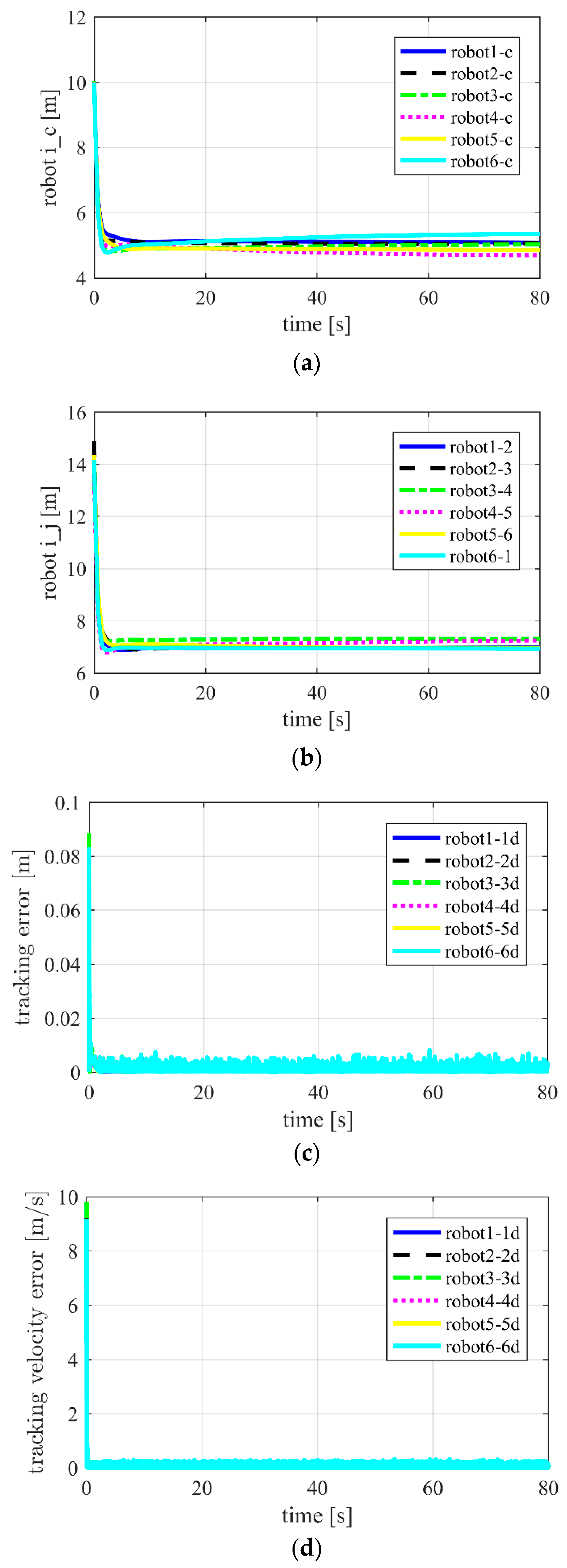
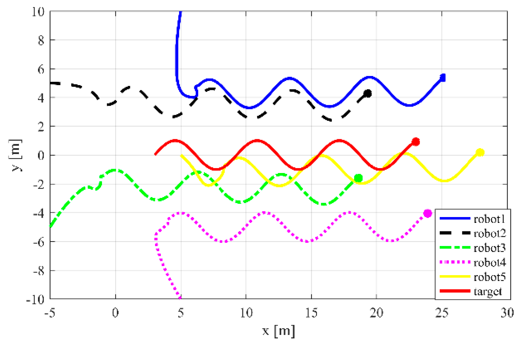
5.2. Case 2: Escorting a Dynamic Target with Constant Velocity

5.2.1. In Two-Dimensional Space

Figure 8 demonstrates the performance of the proposed control algorithm for escorting the target $c={[3+0.1t,0]}^T$.

Next, the effectiveness of the proposed control law is examined when there are two obstacles. The simulation results are presented in Figure 9 and Figure 10, showing that when two obstacles $q_{01}={[15,6]}^T$ and $q_{02}={[25,-5]}^T$ enter the threshold circles of robots 1 and 4, respectively, all of the robots change their positions to avoid the obstacles and collisions.

5.2.2. In Three-Dimensional Space

The simulation experiment results for escorting a target $c={[0.1t,0,0]}^T$ using the proposed law in three-dimensional space are shown in Figure 11 and Figure 12. Figure 13 shows the results when using ASMC. A slower convergence speed and lower control precision are observed compared to when using APD-SMC.

5.3. Case 3: Escorting a Dynamic Target with Time-Varying Velocity

5.3.1. In Two-Dimensional Space

Figure 14 and Figure 15 demonstrate the simulation results for escorting a target $c={[3+0.1t,\sin (0.1t)]}^T$ in two-dimensional space.

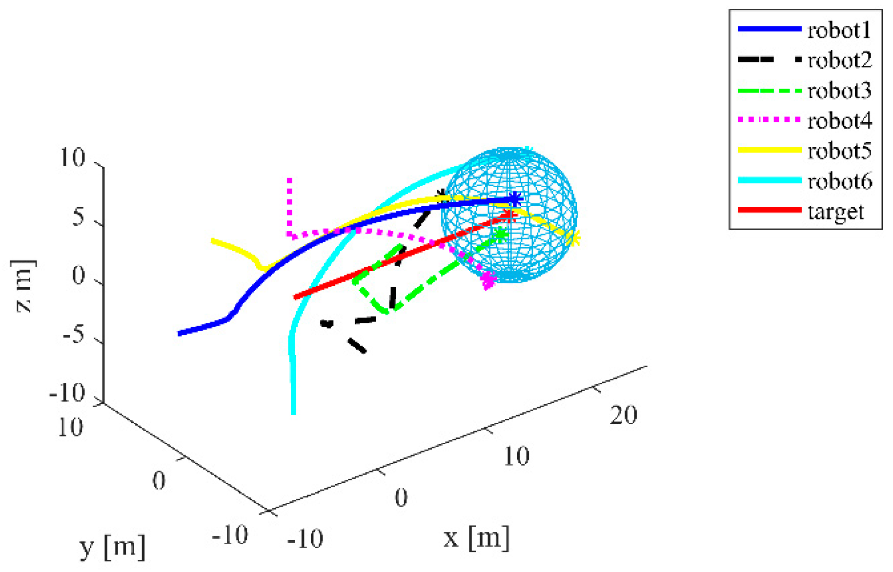
5.3.2. In Three-Dimensional Space

The simulation results for escorting a target $c={[0.1t,\sin (0.1t),0]}^T$ with an obstacle $q_0={\left[15,3,-4.5\right]}^T$ in three-dimensional space as shown in Figure 16 and Figure 17.

In summary, the above simulation results show that the proposed control strategy shows faster and higher control performance than ASMC, and it also provides superior capability while avoiding obstacles.

6. Conclusions

In this study, the coordinated control of multiple Euler–Lagrange systems for escorting missions was investigated in the presence of model uncertainty, disturbances, and obstacles. Our main contribution is the proposal of a robust hierarchical control structure. The NSB controller was proposed in the outer loop to avoid obstacles and escort the target, thus generating the desired velocity for the inner loop. The APD-SMC law was employed in the inner loop to track the desired velocity and ensure fast convergence and robustness. The feasibility of the control scheme was illustrated through Lyapunov theorems and simulation experiment results. Further work will focus on the fault-tolerant coordinated control of multiple Euler–Lagrange systems and the event-based control mechanism for multi-agent systems.

References

1. Huang, J.; Fang, H.; Dou, L.; Chen, J. An overview of distributed high-order multi-agent coordination. IEEE CAA J. Autom. Sin. 2015, 1, 1–9. [Google Scholar]
2. Liu, Y.H.; Xu, Y.S.; Bergerman, M. Cooperation control of multiple manipulators with passive joints. Robot. Autom. IEEE Trans. 1999, 15, 258–267. [Google Scholar]
3. Cheng, L.; Hou, Z.G.; Tan, M. Decentralized adaptive consensus control for multi-manipulator system with uncertain dynamics. In Proceedings of the 2008 IEEE International Conference on Systems, Singapore, 12–15 October 2008; pp. 2712–2717. [Google Scholar]
4. Desai, J.P.; Ostrowski, J.P.; Kumar, V. Modeling and control of formations of nonholonomic mobile robots. IEEE Trans. Robot. Autom. 2002, 17, 905–908. [Google Scholar] [CrossRef]
5. Song, G.; Rui, S.; Li, Y. Cooperative control of multiple nonholonomic robots for escorting and patrolling mission based on vector field. IEEE Access 2018, 6, 41883–41891. [Google Scholar]
6. Yang, Q.; Hao, F.; Mao, Y.; Jie, H. Distributed tracking for networked Euler-Lagrange systems without velocity measurements. J. Syst. Eng. Electron. 2014, 25, 671–680. [Google Scholar] [CrossRef]
7. Mina, H.; Sun, F.; Gao, Z.; Zhang, J. Decentralized adaptive attitude synchronization of spacecraft formation. Syst. Control Lett. 2012, 61, 238–246. [Google Scholar] [CrossRef]
8. Wang, H. Flocking of networked uncertain Euler–Lagrange systems on directed graphs. Automatica 2013, 49, 2774–2779. [Google Scholar] [CrossRef]
9. Mei, J.; Ren, W.; Chen, J.; Guangfu, M.A. Distributed adaptive coordination for multiple Lagrangian systems under a directed graph without using neighbors’ velocity information. Automatica 2013, 49, 1723–1731. [Google Scholar] [CrossRef]
10. Nuño, E.; Ortega, R.; Jayawardhana, B.; Basañez, L. Coordination of multi-agent Euler–Lagrange systems via energy-shaping: Networking improves robustness. Automatica 2013, 49, 3065–3071. [Google Scholar] [CrossRef]
11. Chen, F.; Feng, G.; Liu, L.; Ren, W. Distributed Average Tracking of Networked Euler-Lagrange Systems. Autom. Control IEEE Trans. 2015, 60, 547–552. [Google Scholar] [CrossRef]
12. Meng, Z.; Wei, R.; Zheng, Y. Distributed finite-time attitude containment control for multiple rigid bodies. Automatica 2010, 46, 2092–2099. [Google Scholar] [CrossRef]
13. Ren, W. Distributed leaderless consensus algorithms for networked Euler–Lagrange systems. Int. J. Control 2009, 82, 2137–2149. [Google Scholar] [CrossRef]
14. Antonelli, G.; Arrichiello, F.; Chiaverini, S. The entrapment/escorting mission for a multi-robot system: Theory and experiments. In Proceedings of the IEEE/ASME International Conference on Advanced Intelligent Mechatronics, Zurich, Switzerland, 4–7 September 2007; pp. 1–6. [Google Scholar]
15. Mas, I.; Li, S.; Acain, J.; Kitts, C. Entrapment/escorting and patrolling missions in multi-robot cluster space control. In Proceedings of the IEEE/RSJ International Conference on Intelligent Robots & Systems, St. Louis, MO, USA, 11–15 October 2009; pp. 5855–5861. [Google Scholar]
16. Antonelli, G.; Arrichiello, F.; Chiaverini, S. Stability analysis for the Null-Space-based Behavioral control for multi-robot systems. In Proceedings of the IEEE Conference on Decision & Control, Cancun, Mexico, 9–11 December 2008; pp. 2463–2468. [Google Scholar]
17. Antonelli, G.; Chiaverini, S. Kinematic Control of Platoons of Autonomous Vehicles. IEEE Trans. Robot. 2006, 22, 1285–1292. [Google Scholar] [CrossRef]
18. Antonelli, G.; Arrichiello, F.; Chiaverini, S. The null-space-based behavioral control for autonomous robotic systems. Intell. Serv. Robot. 2008, 1, 27–39. [Google Scholar] [CrossRef]
19. Marino, A.; Parker, L.E.; Antonelli, G.; Caccavale, F. A Decentralized Architecture for Multi-Robot Systems Based on the Null-Space-Behavioral Control with Application to Multi-Robot Border Patrolling. J. Intell. Robot. Syst. 2013, 71, 423–444. [Google Scholar] [CrossRef]
20. Chen, J.; Gan, M.; Huang, J.; Dou, L.; Fang, H. Formation control of multiple Euler-Lagrange systems via null-space-based behavioral control. Sci. China (Inf. Sci.) 2016, 59, 1–11. [Google Scholar] [CrossRef]
21. Antonelli, G.; Arrichiello, F.; Chiaverini, S. The NSB control: A behavior-based approach for multi-robot systems. Paladyn J. Behav. Robot. 2010, 1, 48–56. [Google Scholar] [CrossRef]
22. Slotine, J.J.E.; Li, W. Applied Nonlinear Control; Prentice Hall: Upper Saddle River, NJ, USA, 1991. [Google Scholar]
23. Utkin, V.I. Variable structure systems with sliding modes. IEEE Trans. Autom. Control. 2003, 22, 212–222. [Google Scholar] [CrossRef]
24. Utkin, V.I. Sliding mode control design principles and applications to electric drives. IEEE Trans. Ind. Electron. 2002, 40, 23–36. [Google Scholar] [CrossRef]
25. Lee, K.; Choi, J.; Kim, J. A proportional-derivative-sliding mode hybrid control scheme for a robotic manipulator. Proc. Inst. Mech. Eng. Part 1 J. Syst. Control Eng. 2004, 218, 667–674. [Google Scholar]
26. Ouyang, P.R.; Acob, J.; Pano, V. PD with sliding mode control for trajectory tracking of robotic system. Robot. Comput. Integr. Manuf. 2014, 30, 189–200. [Google Scholar] [CrossRef]
27. Ouyang, P.R.; Pano, V.; Hu, Y.Q. Position domain PD sliding mode control for contour tracking. In Proceedings of the IEEE International Conference on Advanced Intelligent Mechatronics, Busan, Korea, 7–11 July 2015; pp. 1020–1025. [Google Scholar]
28. Yue, W.H.; Pano, V.; Ouyang, P.R.; Hu, Y.Q. Model-independent position domain sliding mode control for contour tracking of robotic manipulator. Int. J. Syst. Sci. 2017, 48, 190–199. [Google Scholar] [CrossRef]
29. Cong, B.L.; Chen, Z.; Liu, X.D. On adaptive sliding mode control without switching gain overestimation. Int. J. Robust Nonlinear Control 2014, 24, 515–531. [Google Scholar] [CrossRef]
30. Ouyang, P.R.; Tang, J.; Yue, W.H.; Jayasinghe, S. Adaptive PD plus sliding mode control for robotic manipulator. In Proceedings of the IEEE International Conference on Advanced Intelligent Mechatronics, Banff, AB, Canada, 12–15 July 2016; pp. 930–934. [Google Scholar]
31. Li, Z.; Ma, X.; Li, Y. Model-free control of a quadrotor using adaptive proportional derivative-sliding mode control and robust integral of the signum of the error. Int. J. Adv. Robot. Syst. 2018, 15, 1–15. [Google Scholar] [CrossRef]
32. Antonelli, G.; Arrichiello, F.; Chiaverini, S. Experiments of Formation Control with Multirobot Systems Using the Null-Space-Based Behavioral Control. IEEE Trans. Control Syst. Technol. 2009, 17, 1173–1182. [Google Scholar] [CrossRef]
33. Zhou, N.; Xia, Y. Coordination control of multiple Euler-Lagrange systems for escorting mission. Int. J. Robust Nonlinear Control 2015, 25, 3596–3616. [Google Scholar] [CrossRef]
34. Huang, J.; Zhou, N.; Cao, M. Adaptive Fuzzy Behavioral Control of Seconde-Order Autonomous Agents with Prioritized Missions: Theory and Experiments. IEEE Trans. Ind. Electron. 2019, 66, 9612–9622. [Google Scholar] [CrossRef]
35. Altschuler, E.L.; Pérez-Garrido, A. Global minimum for Thomson’s problem of charges on a sphere. Phys. Rev. E 2005, 71, 047703. [Google Scholar] [CrossRef]
36. Schwartz, R.E. The five-electron case of Thomson’s problem. Exp. Math. 2013, 22, 157–186. [Google Scholar] [CrossRef]
37. Chiaverini, S. Singularity-robust task-priority redundancy resolution for real-time kinematic control of robot manipulators. Robot. Autom. IEEE Trans. 1997, 13, 398–410. [Google Scholar] [CrossRef] [Green Version]
38. Schlanbusch, R.; Kristiansen, R.; Nicklasson, P.J. Spacecraft formation reconfiguration with collision avoidance. Automatica 2011, 47, 1443–1449. [Google Scholar] [CrossRef]
Figure 1. Block diagram of the overall control system.
Applsci 09 04144 g001
Figure 2. Sketch of null-space-based behavioral (NSB) control with three different tasks.
Applsci 09 04144 g002
Figure 3. Velocity command composition of two tasks.
Applsci 09 04144 g003
Figure 4. The location of six robots and the target in three-dimensional space.
Applsci 09 04144 g004
Figure 5. Using adaptive proportional derivative sliding mode control (APD-SMC) for Case 1 in two-dimensional space. (a) Distances between robot and target q i c ; (b) distances between neighboring robots q i q j ; (c) position tracking error q i q i d ; (d) tracking velocity error q ˙ i q ˙ i d .
Applsci 09 04144 g005aApplsci 09 04144 g005b
Figure 6. Using ASMC for Case 1 in two-dimensional space. (a) Distances between robot and target q i c ; (b) distances between neighboring robots q i q j ; (c) position tracking errors q i q i d ; (d) tracking velocity error q ˙ i q ˙ i d .
Applsci 09 04144 g006aApplsci 09 04144 g006b
Figure 7. The positions of six robots and the target for Case 1 in three-dimensional space.
Applsci 09 04144 g007
Figure 8. Using APD-SMC for Case 2 in two-dimensional space. (a) Distances between robot and target q i c ; (b) distances between neighboring robots q i q j ; (c) position tracking errors q i q i d ; (d) tracking velocity error q ˙ i q ˙ i d .
Applsci 09 04144 g008
Figure 9. The positions of five robots and the target while avoiding obstacles.
Applsci 09 04144 g009
Figure 10. Relative distances between robots and obstacles.
Applsci 09 04144 g010
Figure 11. The positions of six robots and the target for Case 2 in three-dimensional space.
Applsci 09 04144 g011
Figure 12. Using APD-SMC for Case 2 in three-dimensional space. (a) Distances between robot and target q i c ; (b) distances between neighboring robots q i q j ; (c) position tracking error q i q i d ; (d) tracking velocity error q ˙ i q ˙ i d .
Applsci 09 04144 g012
Figure 13. Using ASMC for Case 2 in three-dimensional space. (a) distances between robot and target q i c ; (b) distances between neighboring robots q i q j ; (c) position tracking errors q i q i d ; (d) tracking velocity error q ˙ i q ˙ i d .
Applsci 09 04144 g013
Figure 14. The positions of five robots and the target for Case 3 in two-dimensional space.
Applsci 09 04144 g014
Figure 15. Using APD-SMC for Case 3 in two-dimensional space. (a) Distances between robot and target q i c ; (b) distances between neighboring robots q i q j ; (c) position tracking error q i q i d ; (d) tracking velocity error q ˙ i q ˙ i d .
Applsci 09 04144 g015aApplsci 09 04144 g015b
Figure 16. The positions of six robots and the target while avoiding obstacles.
Applsci 09 04144 g016
Figure 17. Relative distance between the robot and obstacle.
Applsci 09 04144 g017