Featured Application
The constructed Naive Bayes classifier can be used to determine whether or not a tunnel face is stable based on the calculated posterior probability of the stable state with a set of values of the influencing features, making it possible to perform a large number of predictions of tunnel face stability with great efficiency.
Abstract
This paper develops a convenient approach for facilitating the prediction of tunnel face stability in the framework of Bayesian theorem. First, a number of values of the features influencing the face-stability of tunnels are chosen according to the full factorial design. Secondly, the software OptumG2 is utilized to performed strength reduction analyses to obtain safety factors regarding tunnel face stability. Based on the simulated safety factors, the chosen samples are labeled as stable () or unstable samples (). Thirdly, the model parameters that characterize the distribution of the random variables are then estimated by maximizing the well-known likelihood function. After that, the probability density functions (PDF) of the features are identified, and a naive Bayes classifier is constructed with the prior probabilities of the stable and the unstable state. The so-called type I and type II errors are estimated with stable and unstable samples, respectively. The model parameters are then calibrated with additional stable samples to obtain the second classifier. Finally, the two classifiers are evaluated using independent samples that have not been seen in the training dataset. The proposed method allows geotechnical engineers to predict the stability of tunnel faces with great efficiency. It is applicable for general cases of tunnels where the parameters are within the ranges bounded by the specified values.
1. Introduction
Face-stability analysis of tunnels has developed rapidly in recent years. At the construction stage, encountering face collapse is very likely for the tunnels driven in weak ground, such as clay [1], silt, and sand [2,3], and for tunnels with large cross-sectional area [4]. The collapse of the tunnel face threatens the safety of workers, equipment, and adjacent structures, including buildings, bridges, piles [5], underground pipelines, and existing tunnels [6,7]. Design work on the tunnel face involves the evaluation of its stability, the choice of reinforcement measures and the determination of related parameters [8,9,10].
The evaluation process should be conducted primarily to provide suggestions for subsequent design work. If the evaluation result indicates that the tunnel face cannot keep stable itself, it is necessary to take stabilization measures to prevent the collapse. Publications have presented various stabilization measures. For the close face tunneling method, support pressure can be applied via an earth pressure balance machine [11]. For the open face tunneling method, support pressure can be applied by longitudinally installed face bolts [10]. Advanced reinforcement measures, such as forepoling [12] can be used to serve as a beam to reduce the vertical stress acting above the tunnel face. Ground improvement measures are also frequently used to improve the stiffness or strength of soil, aimed at improving the stability of the soil itself [13]. Beyond that, the cross-sectional area is regarded as a crucial factor that influences the stability of a tunnel face. Partial face excavation methods, such as center diaphragm (CD) method, center cross diaphragm (CRD) method, and pile-beam-arch (PBA) method [14], are more favorable than the full-face excavation method regarding the stability of a tunnel face.
The existing methods that have been used for evaluations of tunnel face stability include limit equilibrium [15], limit analysis [16,17], the displacement finite-element method [18], the discrete numerical method [19], scale model test [20,21,22], and centrifuge model test [23,24,25]. These methods have been proven to be useful in determining the limit support pressure and evaluating the effects of reinforcement measures.
However, if the main concern is to figure out whether a tunnel face is stable or not, these methods are either too complicated, or too time-consuming, or both. In fact, there exists an easy-to-use indicator called the stable number, , which can be used to estimate the stability of a tunnel face. In this equation, denotes the surcharge acting on the ground surface, is the unit weight of the soil, H is the depth to tunnel axis, is the support pressure applied at the tunnel face, is the undrained cohesive strength of the ground prior to excavation [26,27,28]. Observations suggested that the tunnel face is deemed to be stable if the stable number is less than or equal to 3 and deemed unstable if the stable number is larger than 6. For cases where the stable number is within the range of 3 to 6, the tunnel faces can be regarded to be in a short-term stable state. Nevertheless, this method is only applicable for purely cohesive soil.
As a result, an easy-to-use and more applicable method is expected to meet the demands of practical engineering, which usually requires a number of evaluations of tunnel face stability with great efficiency due to the varying values of the factors that influence tunnel face stability. Essentially, the task that aims to find out whether a tunnel face is stable or not can be treated as a classification problem, which can be solved by various machine learning algorithms like naive Bayes classifier. This algorithm greatly simplifies learning by assuming that features are independent of each other. Although this assumption may be unrealistic, naive Bayes has found to be effective in practice due to the fact that the classification accuracy may often be correct even if its probability estimates are incorrect [29]. Previous studies proved that the performance of naive Bayes is not directly correlated with the degree of feature dependence [29,30]. This is mainly because the dependencies between features can be ignored when they do not provide information about class [29]. Thus, naive Bayes has been successfully applied to solve various classification problems such as text categorization and automatic medical diagnosis [30,31,32]. It is competitive with other advanced methods including support vector machines because of its convenience and lower computational cost.
Consequently, this paper employed Bayes’ theorem to construct a probabilistic classifier with strong independence assumptions between features to facilitate the predictions of tunnel face stability.
2. Description of the Proposed Method
Figure 1 illustrates the framework of the proposed method. First, four main features that influence tunnel face stability including the cover depth (), the diameter of the tunnel (), the cohesive strength () and the friction angle () of soil are used to constitute a parameter set, . Secondly, different values of parameter sets are chosen using full factorial design within the specified ranges of the features and labeled as stable samples (denoted by +1) or unstable samples (denoted by −1) according to strength reduction analyses. The parameter sets and the corresponding labels will then be combined to create a training dataset, with which a naive Bayes classifier will be constructed with strong independence (naive) assumptions between the four features. Finally, the constructed classifier can be used to classify an unknown sample, , into the stable category if the stable probability is larger than the unstable probability, or into the unstable category if it is not.
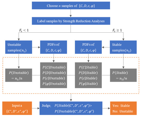
Figure 1.
Framework of the proposed method.
Equation (1) gives the safety factor [33,34,35,36] that can be obtained according to the built-in strength reduction analysis embedded in OptumG2.
where and denote the inputted strength parameters; and denote the critical strength parameters. A factor greater than 1 implies a stable state while a factor less than 1 implies an unstable state that requires ground improvement or additional support pressure to prevent the collapse. With the simulated safety factor, the face-stability of tunnels can be mainly classified into two categories, i.e., (stable) and (unstable).
Bayes’ theorem is a useful tool in the area of statistical analysis [37,38,39]. Researchers have developed many Bayesian methods to solve various geotechnical problems [40,41]. The general expression of the Bayes’ theorem is given as follows:
where A and B denote two events, denotes the conditional probability of event A in the presence of the occurrence of event B. Generally, and are referred to as prior and posterior probabilities, respectively. is the likelihood function that characterizes the probability of the unknown model parameters to be identified with given observed data. The event A can be partitioned into N mutually exclusive events, , and the posterior can be rewritten as:
Relating the event A to the stability of a tunnel face, it can be simply partitioned into two mutually exclusive events, i.e., the stable and the unstable state. The event B accordingly contains the features influencing the face-stability of tunnels, including the cover depth, the diameter of the tunnel, the cohesive strength, and the frictional angle of soil.
Naive Bayesian is a conditional probability model that can be used to formulate classifiers. It is based on the assumption that the value of a feature is independent of the value of the others. Accordingly, the posterior probability of an event can be expressed as follows:
where the vector represents some n features that are assumed to be independent with each other, represents the nth possible outcome of class. Using Bayes’ theorem, the conditional probability can be decomposed as follows:
Using Bayesian probability terminology, Equation (5) can be rewritten as:
If we choose as the associated features influencing the face-stability of tunnels, the posterior probabilities concerning the stable and unstable states can be expressed as:
where evidence is a normalization constant that can be calculated as:
A naive Bayes classifier can be constructed by synthesizing the naive Bayes probability model and a decision rule. One common rule is the well-known maximum a posteriori (MAP) decision rule. Under this circumstance, the prediction of a tunnel face stability can be accordingly performed such that indicates a stable state while indicates an unstable state.
Using the evidence, the posterior probabilities of the events are normalized and their sum becomes 1, as shown in Equation (10). In conjunction with MAP decision rule, the posterior probabilities of the events can be employed to classify the stable and unstable states such that and represent a stable state, and represent an unstable state.
With the number of the stable samples (denoted by ) and unstable samples (denoted by ), the prior probabilities of the stable and unstable states can be determined as follows:
Beyond that, the model parameters, i.e., expectations and standard deviations, were estimated and calibrated by the well-known maximum likelihood functions before the identification of the probability density functions of the related features. After that, it is possible to calculate the likelihood (i.e., ) of each feature. A naive Bayes classifier was subsequently constructed based on the identified prior probabilities, as well as the calculated likelihood of each feature. The posterior probabilities of the stable and unstable states can be calculated with a given set of values of the features. It enables the prediction of the face-stability of tunnels by comparing the values of the two posterior probabilities.
3. Application Example
This section presents an application example to illustrate the framework of the proposed method. In addition to the four features mentioned above, there are several other features that can affect tunnel face stability, such as the unit weight of soil, the surcharge load located on the ground surface, and the underground water. However, it is difficult to take all the influences into account simultaneously. Consequently, several simplifications have been made.
The surcharge load was not included because existing literature found that this type of load has neglect effects on tunnel face stability when the ratio of the cover depth to the diameter of the tunnel is larger than 0.6. The underground water was not considered due to the fact that in most cases the tunnel face is unstable in the presence of underground water. As a result, the method aims to predict the stability of a tunnel face for cases where the underground water table is lower than the bottom of the tunnel, or for cases where dewatering measures have been taken to lower the underground water table before the excavation stage. The unit weight of the soil was considered to be a relatively large constant, 19 kN/m3. Under this circumstance, the prediction results are conservative for cases where the unit weights of the soil are less than 19 kN/m3.
With these simplifications, a number of tunnels with cover depth , and diameter were considered to be driven in a soil molded as an isotropic Mohr–Coulomb material with cohesive strength , and friction angle . General cases of tunnels are within the ranges bounded by the specified values, beyond which are cases which usually require special analyses. For example, if the diameter of a tunnel exceeds , it can be taken as a large cross-section tunnel.
Among these factors, it is well known that cohesion and friction angle are correlated. Herein, we assumed that these two parameters are independent of each other to be in accordance with the assumption of the naive Bayes classifier. In fact, the naive Bayes Classifier has been used to solve many classification problems that involve correlated factors. Despite the assumption, naive Bayes Classifier is still competitive when compared to other algorithms because of its convenience, lower computational cost, and comparable performance [29,32,42].
Figure 2 gives the diagram of the numerical models, including the geometry parameters and the boundary conditions. Normal fixities were applied on the left and right boundaries to constrain the horizontal displacements while full fixities were applied on the bottom boundary to constrain both the vertical and horizontal displacements.
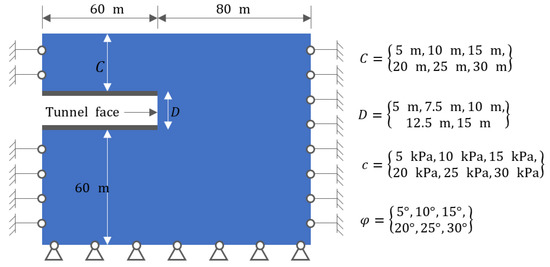
Figure 2.
Numerical model and boundary conditions.
In terms of full factorial design, the number of the features and the corresponding levels presented in Figure 2 involves combinations regarding the cover depths and the diameters. This means that 30 numerical models are needed. In conjunction with the number of the values associated with the cohesive strength (5) and the friction angle (5), the total number of strength reduction analyses can be identified as follows:
It should be emphasized that tunnel face stability is more appropriate to be analyzed in 3D simulations, which may be performed using OptumG3. However, the reality is that OptumG3 has not yet provided a built-in strength reduction analysis function. As a result, the strength reduction process needs to be conducted manually rather than automatically. This requires huge computational cost, particularly when there are 750 3D numerical models to be constructed and simulated. The total number of 3D simulations may reach up to several thousand because each case involves several or even many tries to determine the safety factor. This means that it is extremely difficult to obtain 3D safety factors for constructing a naive Bayes classifier. Thus, this paper utilizes 2D upper bound analysis with associated flow rule to complete the task of collecting training samples.
In fact, the 2D failure mechanism of tunnel face stability has been developed and used in the existing literature to obtain approximate solutions [27,43]. Moreover, twenty cases with different values of features are used to perform both 2D (automatically) and 3D (manually) strength reduction analyses. The comparison results shown in Figure 3 imply that 2D simulations may give relatively good and conservative approximations of 3D safety factors.
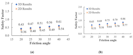
Figure 3.
Comparison of safety factors computed in 2D and 3D simulations: (a) ; (b) ; (c) ; (d) .
Note that the main purpose of strength reduction analysis is to figure out whether or not a tunnel face is stable, rather than to assess the degree of safety (or stability). This means that only a few samples with 2D safety factors varying between 0.8 to 1.0 (based on Figure 3) may cause adverse effects on subsequent prediction accuracy of the classifier since these samples may be stable in 3D simulations but will be misclassified into the unstable category according to the simulated 2D safety factors. In most cases, this type of approximation error will not cause any prediction error as long as the 2D and 3D safety factors represent the same state of stability (i.e., both stable or both unstable).
However, 3D simulations are still expected in the near future to obtain a large number of high-accuracy safety factors, if strength reduction analyses of various cases can be run programmatically in OptumG3.
For the cases with and , the simulated safety factors were collected and listed in Table 1, in which the safety factors greater than 1.0 were indicated with red dashed rectangles. As mentioned above, the 25 samples can be classified into 7 stable samples and 18 unstable samples according to the simulated safety factors.

Table 1.
Calculated strength reduction factors with and .
Similarly, the other 725 strength reduction analyses were performed, and the collected safety factors are plotted versus the reference numbers and shown in Figure 4, in which a red dashed line with was added to classified the collected samples into two categories, i.e., 45 stable samples and 705 unstable samples. Thus, the prior probabilities of the stable and unstable states are available:
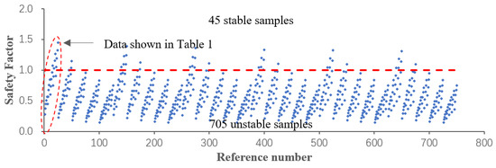
Figure 4.
Simulated safety factors of the 750 samples.
4. Estimation of Model Parameters
With the given values of the features, as well as the classifications determined by the simulated safety factors, model parameters associated with the probability density functions of the features can be identified using the so-called maximum likelihood principles. To achieve this, let D denote the observed data, and let denote the parameters of an unknown model to be estimated and calibrated. The well-known likelihood function is generally expressed as , which is always converted to the log-likelihood function for facilitating the evaluation of its maximization, based on which the equation can be easily solved to yield the optimal value of . Suppose the values of the four features influencing the stability of a tunnel face follow the normal distribution. The means and standard deviations of these values (denoted as and ) need to be estimated to identify the probability density function.
Let denote the n inputted values of the buried depth; its likelihood function can be expressed as:
The log-likelihood of which can be rewritten as:
The optimal values of and can be determined by equating the gradients of the above equation with respect to and , respectively, to zero, as shown in Equations (17) and (18).
where and denote the maximum likelihood estimations of and , respectively. According to the above equations, the optimal values of the model parameters relating to inputted values of the cover depth are , and , respectively, as listed in Table 2, in which the maximum likelihood estimations of the model parameters of the other three features were similarly identified.
Table 2.
Parameters associated with probability density function (PDF, the first classifier).
The PDFs of the buried depth associated with the stable state and the unstable state are of the type:
The other PDFs that characterize the distribution of the features can be identified in the same way, as plotted and shown in Figure 5.
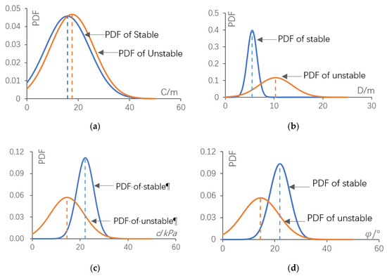
Figure 5.
PDF of parameters for stable and unstable samples: (a) the cover depth; (b) the diameter; (c) the cohesive strength; (d) the friction angle.
Results in Figure 5 show that the PDF of the cover depth of the stable samples is very close to that of the unstable samples. This is mainly because of the so-called arch effect, which can serve to support most of the vertical stress acting above the tunnel face, resulting in a decrease in the horizontal stress that induces the collapse of the tunnel face. Conversely, the PDF of the diameter of the stable samples differs substantially with that of the unstable samples, which indicates that the tunnel diameter is the most crucial influencing factor. The difference between the PDFs of the cohesive strength for the stable and the unstable samples is similar to that of the friction angle because the values of these two features are always divided by the same reduction in strength reduction analyses.
5. Prediction of Stability and Estimation of Errors
Together with the identified PDFs, a naive Bayes classifier (referred to as the first classifier subsequently) can be constructed with the calculated prior probabilities. If we consider a tunnel with , the stable and unstable probability of the given value of the cover depth, , can be calculated based on its PDFs:
Similarly, the values of the other probabilities can be calculated according to the PDFs of the features as:
The normalized constant can be identified as:
The posterior probability of the stable state is calculated as:
And the posterior probability of the unstable state is:
As mentioned above, the face-stability of the tunnel with the calculated can be concluded to be stable. For verification, a 2D numerical model was built with OptumG2 to perform a Strength Reduction analysis with the same values of the features. Figure 6 shows the adaptive mesh of the model, including the geometry parameters, strength parameters, and the boundary conditions. Normal fixities were applied on the boundary of the excavated element to serve as the temporary lining.
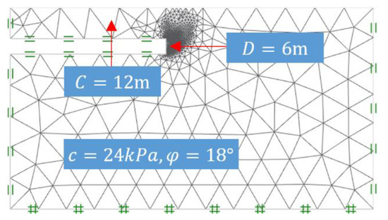
Figure 6.
Strength reduction analysis for verification.
The simulated safety factor is , which means that a limit state can be achieved if the strength parameters and are adopted in an analysis while the other conditions remain constant. In other words, it indicates a stable state with , verifying the above prediction.
In the same way, the error rate of the constructed naive Bayes classifier can be estimated with the entire training data. The estimation results are indicated in Figure 7, where two red dashed lines with the posterior probability equal to 0.5 are added as baselines to distinguish the error estimations, as located below the baseline.
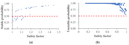
Figure 7.
Error estimation for the first classifier. (a) Stable probability of the samples with ; (b) unstable probability of the samples with .
Results in Figure 7 show that 18 of the 45 stable samples were predicted to be unstable. The error rate estimated for the stable samples (40%) is the well-known indicator of type I error, which is an underestimation of the face-stability. The safety factors of the error estimations range from 1.01 to 1.15, which indicates that type I error is more likely to happen when the face-stability of a tunnel is close to the limit state, i.e., . On the contrary, type II error is an overestimation of the face-stability. Fortunately, the posterior probabilities of the unstable samples show no points located below the baseline, indicating that the rate of type II error is zero. This is mainly because the number of the stable samples is much less than that of the unstable samples. As a result, we extended the ranges of the strength parameters with two higher values, i.e., , intended to obtain additional stable samples to reduce the rate of type I error.
For samples with safety factors greater than 1.0, the material parameters were increased to high levels to obtain new stable samples. For example, if a sample with and is stable, samples with , or , or , or are also stable (geometry parameters remains constant). In such a manner, 52 additional samples were obtained and labeled according to strength reduction analyses, as shown in Figure 8.
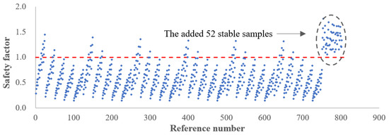
Figure 8.
Strength reduction factors with additional samples.
With these extra 52 stable samples, the number of stable samples becomes , the number of unstable samples remains , while the total number of samples increases to . As a result, the prior probability of the stable and unstable states can be altered:
Table 3 summarizes the calibrated model parameters associated with the PDFs of the features. Another naive Bayes classifier (referred to as the second classifier subsequently) was constructed with the PDFs (Figure 9) of the features, as well as the recalculated prior probabilities. Note that the model parameters relating to the unstable samples remain constant while those relating to the stable samples changed slightly due to the additional stable samples.
Table 3.
Parameters associated with PDF (the second classifier).
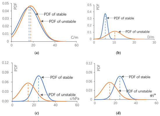
Figure 9.
Updated PDFs of features with extra stable samples: (a) the cover depth; (b) the diameter; (c) the cohesive strength; (d) the friction angle.
Error estimation of the second classifier was performed in the same way. The results in Figure 10 demonstrate that the rate of type I error decreases substantially from 40% to 6%, and the rate of type II error increases from 0% to 0.28%. If necessary, adding other samples can further improve the accuracy of the classifier.
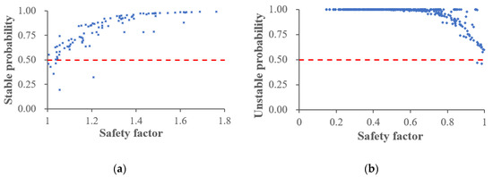
Figure 10.
Error estimation for the second classifier. (a) Stable probability of the samples with ; (b) unstable probability of the samples with .
To check the validation of the constructed classifiers, 50 new samples were randomly chosen and labeled according to strength reduction analyses. The calculated stable or unstable probabilities of the samples are plotted vs. the simulated safety factors and shown in Figure 11 and Figure 12. As can be seen, most of the test samples can be correctly classified, and the 2nd classifier performs much better than the first one regarding both stable and unstable samples. This is consistent with the conclusion obtained from the error estimations of the two classifiers using the training dataset.
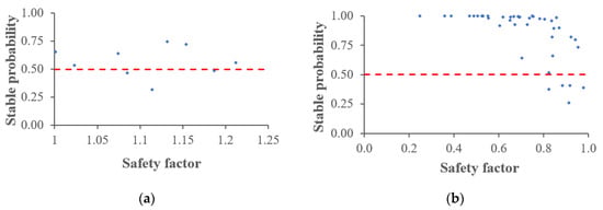
Figure 11.
Prediction of the test data using the first classifier. (a) Stable probability of the samples with ; (b) unstable probability of the samples with .
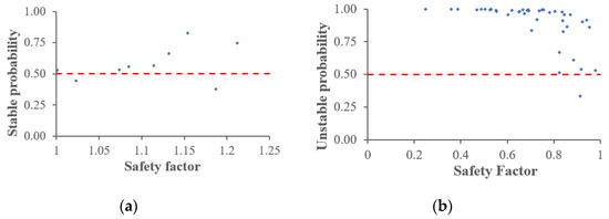
Figure 12.
Prediction of the test data using the second classifier. (a) Stable probability of the samples with ; (b) unstable probability of the samples with .
Consequently, the 2nd naive Bayesian classifier is recommended for initial predictions of tunnel face stability. A number of predictions can be readily conducted using Equations (7) and (8) based on the determined statistical parameters of the four influencing factors. The constructed classifier serves like an empirical formula, allowing geotechnical engineers to evaluate tunnel face stability with great efficiency during the construction stage.
6. Conclusions
This paper developed a convenient method for the prediction of tunnel face stability using the naive Bayes classifier. A number of samples were chosen to be labeled according to strength reduction analyses and were then used to construct a naive Bayes classifier for predictions of tunnel face stability from the perspective of probability. The method makes it possible to conduct a number of predictions with great efficiency. Based on the above study, several conclusions can be drawn:
- The constructed classifiers have acceptable prediction accuracies on both the training and test datasets even though the factors were assumed to be independent. The validation results prove the feasibility of the prosed method that predicts the stability of a tunnel face from the perspective of probability.
- The constructed naive Bayes classifier is time-efficient in the initial evaluations of the face-stability of tunnels. The collapse of a tunnel face will occur if and will not occur if . For the case of unstable faces, reinforcement or support measures are required to prevent the collapse.
- The error estimation indicates that the error rate highly relies on the number of samples adopted for the determination of the prior probabilities and the PDFs of the features. The second classifier is recommended for initial predictions of tunnel face stability because it performs much better than the first one. If it is necessary, the classifiers can be further calibrated to be more sophisticated by adding more stable samples to reduce the imbalance between the number of stable and unstable samples. Type error is relatively high but conservative, while Type error is extremely low but is more serious since it induces an overestimation of the face-stability.
- It is more likely to encounter an error when a safety factor approximates to 1.0 or a posterior probability approximates to 0.5 (i.e., the limit state). As a result, is strongly recommended for further verifications by other means to avoid both type error and type error.
- The naive Bayes classifier is constructed based on 2D simulation results because the task of collecting a large number of 3D safety factors is very difficult presently, particularly when the function of strength reduction analysis is not yet included in OptumG3. It appears that 2D strength reduction analyses can yield close and conservative approximations of 3D safety factors. Indeed, 2D results also have good reliability if the main purpose is only to figure out whether or not a tunnel face is stable. However, since tunnel face stability is an intrinsic 3D problem, the prediction reliability of the classifier is expected to be improved by replacing the training samples with 3D simulation results as long as numerous 3D strength reduction analyses can be run programmatically.
Author Contributions
Funding acquisition, B.L. and H.L.; Investigation, H.L.; Methodology, B.L. and H.L.; Validation, B.L.; Writing—original draft, B.L.
Funding
The study is supported by the National Natural Science Foundation of China (No.51608407), the China Scholarship Council (No. 201706955065), and the project from the Department of Transportation of Hubei Province (No. 2011-700-2-22).
Conflicts of Interest
The authors declare no conflicts of interest.
References
- Hong, Y.; Ng, C.W.W.; Wang, L.Z. Initiation and failure mechanism of base instability of excavations in clay triggered by hydraulic uplift. Can. Geotech. J. 2014, 52, 599–608. [Google Scholar] [CrossRef]
- Liu, W.; Zhao, Y.; Shi, P.; Li, J.; Gan, P. Face stability analysis of shield-driven tunnels shallowly buried in dry sand using 1-g large-scale model tests. Acta Geotech. 2018, 13, 693–705. [Google Scholar] [CrossRef]
- Lü, X.; Zhou, Y.; Huang, M.; Zeng, S. Experimental study of the face stability of shield tunnel in sands under seepage condition. Tunn. Undergr. Space Technol. 2018, 74, 195–205. [Google Scholar] [CrossRef]
- Bandini, A.; Berry, P.; Cormio, C.; Colaiori, M.; Lisardi, A. Safe excavation of large section tunnels with Earth Pressure Balance Tunnel Boring Machine in gassy rock masses: The Sparvo tunnel case study. Tunn. Undergr. Space Technol. 2017, 67, 85–97. [Google Scholar] [CrossRef]
- Hong, Y.; Soomro, M.A.; Ng, C.W.W. Settlement and load transfer mechanism of pile group due to side-by-side twin tunnelling. Comput. Geotech. 2015, 64, 105–119. [Google Scholar] [CrossRef]
- Gue, C.Y.; Wilcock, M.J.; Alhaddad, M.M.; Elshafie, M.Z.E.B.; Soga, K.; Mair, R.J. Tunnelling close beneath an existing tunnel in clay–perpendicular undercrossing. Géotechnique 2017, 67, 795–807. [Google Scholar] [CrossRef]
- Khattri, S.K.; Log, T.; Kraaijeveld, A. Tunnel Fire Dynamics as a Function of Longitudinal Ventilation Air Oxygen Content. Sustainability 2019, 11, 203. [Google Scholar] [CrossRef]
- Rasouli, M. Engineering geological studies of the diversion tunnel, focusing on stabilization analysis and support design, Iran. Eng. Geol. 2009, 108, 208–224. [Google Scholar] [CrossRef]
- Bin, L.; Taiyue, Q.; Wang, Z.; Longwei, Y. Back analysis of grouted rock bolt pullout strength parameters from field tests. Tunn. Undergr. Space Technol. 2012, 28, 345–349. [Google Scholar] [CrossRef]
- Li, B.; Hong, Y.; Gao, B.; Qi, T.Y.; Wang, Z.Z.; Zhou, J.M. Numerical parametric study on stability and deformation of tunnel face reinforced with face bolts. Tunn. Undergr. Space Technol. 2015, 47, 73–80. [Google Scholar] [CrossRef]
- Dias, D.; Kastner, R. Movements caused by the excavation of tunnels using face pressurized shields—Analysis of monitoring and numerical modeling results. Eng. Geol. 2013, 152, 17–25. [Google Scholar] [CrossRef]
- Juneja, A.; Hegde, A.; Lee, F.H.; Yeo, C.H. Centrifuge modelling of tunnel face reinforcement using forepoling. Tunn. Undergr. Space Technol. 2010, 25, 377–381. [Google Scholar] [CrossRef]
- Dwivedi, R.D.; Singh, M.; Viladkar, M.N.; Goel, R.K. Prediction of tunnel deformation in squeezing grounds. Eng. Geol. 2013, 161, 55–64. [Google Scholar] [CrossRef]
- Liu, J.; Wang, F.; He, S.; Wang, E.; Zhou, H. Enlarging a large-diameter shield tunnel using the Pile–Beam–Arch method to create a metro station. Tunn. Undergr. Space Technol. 2015, 49, 130–143. [Google Scholar] [CrossRef]
- Sloan, S.W. Geotechnical stability analysis. Geotech. Lond. 2013, 63, 531–572. [Google Scholar] [CrossRef]
- Leca, E.; Dormieux, L. Upper and lower bound solutions for the face stability of shallow circular tunnels in frictional material. Géotechnique 1990, 40, 581–606. [Google Scholar] [CrossRef]
- Xiang, Y.; Song, W. Upper-Bound Limit Analysis of Shield Tunnel Stability in Undrained Clays Using Complex Variable Solutions for Different Ground-Loss Scenarios. Int. J. Geomech. 2017, 17, 04017057. [Google Scholar] [CrossRef]
- Paternesi, A.; Schweiger, H.F.; Scarpelli, G. Numerical analyses of stability and deformation behavior of reinforced and unreinforced tunnel faces. Comput. Geotech. 2017, 88, 256–266. [Google Scholar] [CrossRef]
- Zhang, Z.X.; Hu, X.Y.; Scott, K.D. A discrete numerical approach for modeling face stability in slurry shield tunnelling in soft soils. Comput. Geotech. 2011, 38, 94–104. [Google Scholar] [CrossRef]
- Shin, J.H.; Choi, Y.K.; Kwon, O.Y.; Lee, S.D. Model testing for pipe-reinforced tunnel heading in a granular soil. Tunn. Undergr. Space Technol. 2008, 23, 241–250. [Google Scholar] [CrossRef]
- Ahmed, M.; Iskander, M. Evaluation of tunnel face stability by transparent soil models. Tunn. Undergr. Space Technol. 2012, 27, 101–110. [Google Scholar] [CrossRef]
- Chen, R.; Li, J.; Kong, L.; Tang, L. Experimental study on face instability of shield tunnel in sand. Tunn. Undergr. Space Technol. 2013, 33, 12–21. [Google Scholar] [CrossRef]
- Kamata, H.; Mashimo, H. Centrifuge model test of tunnel face reinforcement by bolting. Tunn. Undergr. Space Technol. 2003, 18, 205–212. [Google Scholar] [CrossRef]
- Idinger, G.; Aklik, P.; Wu, W.; Borja, R.I. Centrifuge model test on the face stability of shallow tunnel. Acta Geotech. 2011, 6, 105–117. [Google Scholar] [CrossRef]
- Wong, K.S.; Ng, C.W.W.; Chen, Y.M.; Bian, X.C. Centrifuge and numerical investigation of passive failure of tunnel face in sand. Tunn. Undergr. Space Technol. 2012, 28, 297–303. [Google Scholar] [CrossRef]
- Pinyol Núria, M.; Alonso Eduardo, E. Design of Micropiles for Tunnel Face Reinforcement: Undrained Upper Bound Solution. J. Geotech. Geoenviron. Eng. 2012, 138, 89–99. [Google Scholar] [CrossRef]
- Zhang, Z.; Shi, X.; Wang, B.; Li, H. Stability of NATM tunnel faces in soft surrounding rocks. Comput. Geotech. 2018, 96, 90–102. [Google Scholar] [CrossRef]
- Ukritchon, B.; Yingchaloenkitkhajorn, K.; Keawsawasvong, S. Three-dimensional undrained tunnel face stability in clay with a linearly increasing shear strength with depth. Comput. Geotech. 2017, 88, 146–151. [Google Scholar] [CrossRef]
- Rish, I. An empirical study of the naive Bayes classifier. J. Universal Comput. Sci. 2001, 1, 127. [Google Scholar]
- Domingos, P.; Pazzani, M. On the Optimality of the Simple Bayesian Classifier under Zero-One Loss. Mach. Learn. 1997, 29, 103–130. [Google Scholar] [CrossRef]
- Mitchell, T.M. Machine Learning, 1st ed.; McGraw-Hill, Inc.: New York, NY, USA, 1997. [Google Scholar]
- McCallum, A.; Nigam, K. A comparison of event models for naive bayes text classification. In Proceedings of the AAAI-98 Workshop on Learning for Text Categorization, Madison, WI, USA, 26–27 July 1998; pp. 41–48. [Google Scholar]
- Tu, Y.; Liu, X.; Zhong, Z.; Li, Y. New criteria for defining slope failure using the strength reduction method. Eng. Geol. 2016, 212, 63–71. [Google Scholar] [CrossRef]
- Park, D.; Michalowski, R.L. Three-dimensional stability analysis of slopes in hard soil/soft rock with tensile strength cut-off. Eng. Geol. 2017, 229, 73–84. [Google Scholar] [CrossRef]
- Pan, Q.; Dias, D. Upper-bound analysis on the face stability of a non-circular tunnel. Tunn. Undergr. Space Technol. 2017, 62, 96–102. [Google Scholar] [CrossRef]
- Pan, Q.; Dias, D. Safety factor assessment of a tunnel face reinforced by horizontal dowels. Eng. Struct. 2017, 142, 56–66. [Google Scholar] [CrossRef]
- Cao, Z.; Wang, Y. Bayesian approach for probabilistic site characterization using cone penetration tests. J. Geotech. Geoenviron. Eng. 2012, 139, 267–276. [Google Scholar] [CrossRef]
- Cao, Z.; Wang, Y. Bayesian model comparison and characterization of undrained shear strength. J. Geotech. Geoenviron. Eng. 2014, 140, 04014018. [Google Scholar] [CrossRef]
- Cao, Z.; Wang, Y. Bayesian model comparison and selection of spatial correlation functions for soil parameters. Struct. Saf. 2014, 49, 10–17. [Google Scholar] [CrossRef]
- Wang, Y.; Au, S.K.; Cao, Z. Bayesian approach for probabilistic characterization of sand friction angles. Eng. Geol. 2010, 114, 354–363. [Google Scholar] [CrossRef]
- Wang, Y.; Cao, Z.; Li, D. Bayesian perspective on geotechnical variability and site characterization. Eng. Geol. 2016, 203, 117–125. [Google Scholar] [CrossRef]
- Ng, A.Y.; Jordan, M.I. On discriminative vs. generative classifiers: A comparison of logistic regression and naive bayes. In Advances in Neural Information Processing Systems; MIT Press: Cambridge, MA, USA, 2001; pp. 841–848. [Google Scholar]
- Mollon, G.; Phoon, K.K.; Dias, D.; Soubra, A. Validation of a New 2D Failure Mechanism for the Stability Analysis of a Pressurized Tunnel Face in a Spatially Varying Sand. J. Eng. Mech. 2011, 137, 8–21. [Google Scholar] [CrossRef]
© 2019 by the authors. Licensee MDPI, Basel, Switzerland. This article is an open access article distributed under the terms and conditions of the Creative Commons Attribution (CC BY) license (http://creativecommons.org/licenses/by/4.0/).