Sediment Erosion Characteristics and Mechanism on Guide Vane End-Clearance of Hydro Turbine

Abstract

Sediment erosion caused by the collision of solid particles is a challenge for the safety, reliability, unit efficiency, and vibration noise of the hydroelectric engineering system located at China’s Yellow River and northwest inland basin. The sediment-laden flow of the guide vane end-clearance of the Francis Turbine at Dongshuixia hydroelectric station was used as the research object, and the large eccentric shaft structure of a guide vane was considered. Numerical calculations with the large eddy simulation (LES) and discrete phase models (DPMs) were carried out to study the erosion characteristics and mechanism of the end-surface of the guide vane and head cover, the flow mechanism of adverse erosion behind the shaft, and the influence law of the turbulence integral scale, turbulent kinetic energy, and turbulent flow angle on erosion. The flow field with a 1 mm clearance should set the number of particle trajectory per unit inlet area at about 1/mm² to ensure the accuracy of calculation. The von Kármán vortex street is the main reason for adverse erosion behind the shaft and the low frequency energy of the turbulence plays a leading role in erosion. The above results provide a reference for the optimization design of an anti-wear guide vane and wear-protection of the clearance with sediment-laden water.

1. Introduction

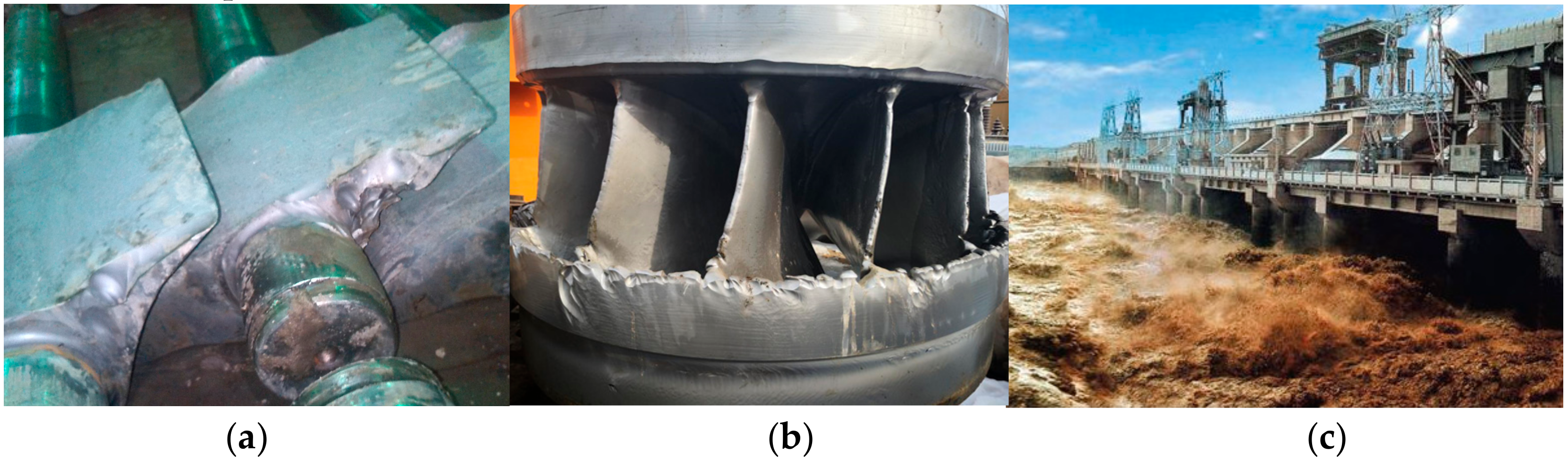
China is rich in water energy resources. The country’s outstanding features include precipitous watercourses with a concentrated distribution for climate, its topography and other factors, which are very beneficial to the development of hydropower [1]. According to statistical data from the National Energy Administration, by the end of 2018, the total hydropower installed capacity and annual energy output in China were up to 350 GW and 1200 TWh, respectively. All natural water resources carry impurities such as suspended sediment and solid particulates. For hydro turbines working in the natural environment, flow problems can be classified as complex multiphase flow. In the China’s Yellow River and northwest inland basin, the running hydroelectric project suffers from maintenance challenges as sediment causes erosion of the flow passage components of the turbines (see Figure 1). The energy loss caused by the outage or maintenance of the hydro turbine flow passage parts due to erosion is about 2–3 TWh each year, and the annual maintenance cost and renewal cost of equipment is hundreds of millions of yuan.

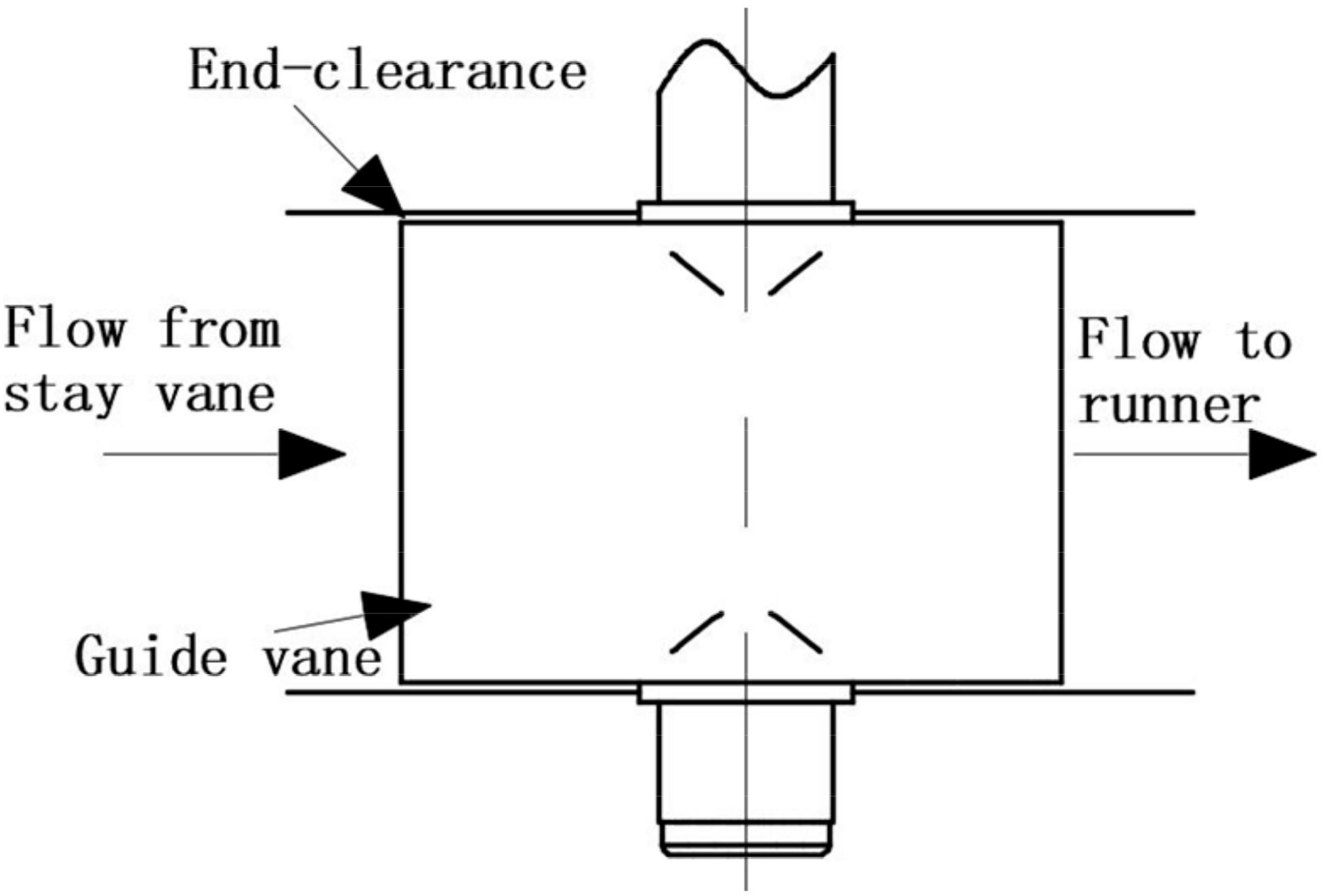
Guide vanes direct the sediment-laden water onto the runner blades at a suitable angle, thus providing a tangential velocity and an angular momentum to the sediment-laden water. Furthermore, a small end-clearance is designed at the upper and lower surface of the guide vane, allowing them to be pivoted to regulate the flow (see Figure 2) [2]. Turbines experience several unsteady sediment-laden flows where such flows contribute to erosion in the flow-passage walls of the guide vane clearance. The enlarged clearance would lead to changes in the flow pattern, increases in water leakage, losses in efficiency and output power, vibration, and even the final breakdown of the turbine components [3,4].

A number of detailed studies of the flow field around guide vanes and end-clearance flow have been undertaken by many scholars. A theoretical and experimental study of flow through the double cascade of a Francis turbine was conducted by Chen et al. [5] who observed the flow around guide vanes with different sizes of end-clearance, where a crosswise leakage flow developed from the end-clearance due to the pressure gradient between the guide vane surfaces. An experimental apparatus with a cascade of guide vanes in a Francis turbine was developed by Thapa et al. [6,7,8] who observed leakage flow as a jet flow, which was mixed with the mainstream in the transverse direction and then formed a vortex. Therefore, the inlet flowrate of runner blades will be uneven.

In the aspect of numerical simulations studies, Koirala et al. [9] used the Tabakoff erosion model to analyze the erosion in Francis turbines and studied the effect of the guide vane clearance gap on Francis turbine performance. A very thorough numerical investigation detailed by Tallman et al. [10] showed the influence of clearance size on the leakage flow, vortex, and secondary flow. Noon et al. [11] used the k-omega based Shear-Stress-Transport (SST) model and the Finnie and Tabakoff erosion models in ANSYS CFX to studied flow field and erosion wear on Francis Turbine components due to sediment flow, who found that erosion and efficiency loss both decreases with increase in particle shape factor. Messa et al. [12] used a volume of fluid (VOF) model for simulating the free nozzle jet, a Lagrangian particle tracking model for the trajectories of the solid particles, and Oka and det norske veritas (DNV) models for estimating the mass removal. A previously validated multiscale model of erosion is presented by Leguizamón et al. [13,14] to obtain erosion distribution and the erosion process of Pelton bucket impacted by a sediment-laden water jet. This model consists of two coupled sub-models. The sediment impacts are simulated by means of comprehensive physical models on the microscale and turbulent sediment transport and erosion accumulation are calculated on the macroscale. Brekke [15] studied the mechanisms of sediment erosion at guide vanes, where erosion was categorized as turbulence erosion, secondary flow erosion, leakage erosion, and acceleration erosion. In addition, the influence of end-clearance on turbine efficiency was studied, where the loss in efficiency is greater than the increase of leakage flow. Koirala [16] showed that high quartz content, inefficiency of the flushing system, higher concentration of sediment load, high impingement velocity, and operation at low guide vane angles were the major contributors to sediment erosion in guide vanes. The end-surface clearance flow of the turbine guide vane was simplified as circular-cylinder flow and backward-facing step flow by Han [17,18,19]. The erosion of the flow-passage walls with inlet velocity, particle diameter, and particle density has been studied by the discrete phase model (DPM) and mixture model, and the sediment-wear morphology prediction method based on the differential-quadrature method has been proposed.

Through a comparison and analysis of the above references, few studies have been conducted on the turbulence characteristics and erosional mechanism at the end-clearance flow of guide vanes with a large eccentric shaft. This paper used the end-clearance flow of the turbine guide vanes with a large eccentric shaft at the Dongshuixia hydropower station as the research object, and simulated the flow in the clearance and around the guide vane with a large eddy simulation (LES) and discrete phase model (DPM). Using the actual wear pattern of the unit, the turbulence characteristics and the wear mechanism of the guide vane were analyzed and studied.

2. Sediment Erosion Status of Dongshuixia Hydropower Station

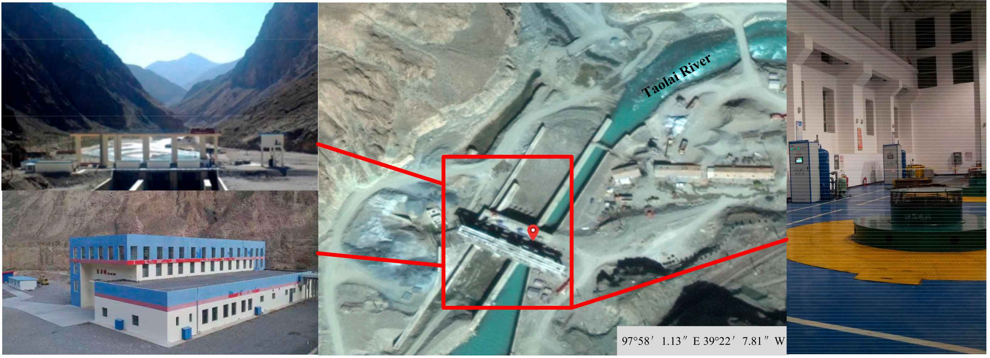
The Dongshuixia hydropower station is a water diversion and electric generating project with a low-clam long tunnel, and is located at the main stream canyon segment of the Taolai river in Sunan County of Gansu Province (see Figure 3). The average annual generated energy is up to 2.43 billion kW·h. This project was completed and put into operation in July 2012, which was of great significance to improve the local network structure, palliate the power shortage, and promote the development of the local economy.

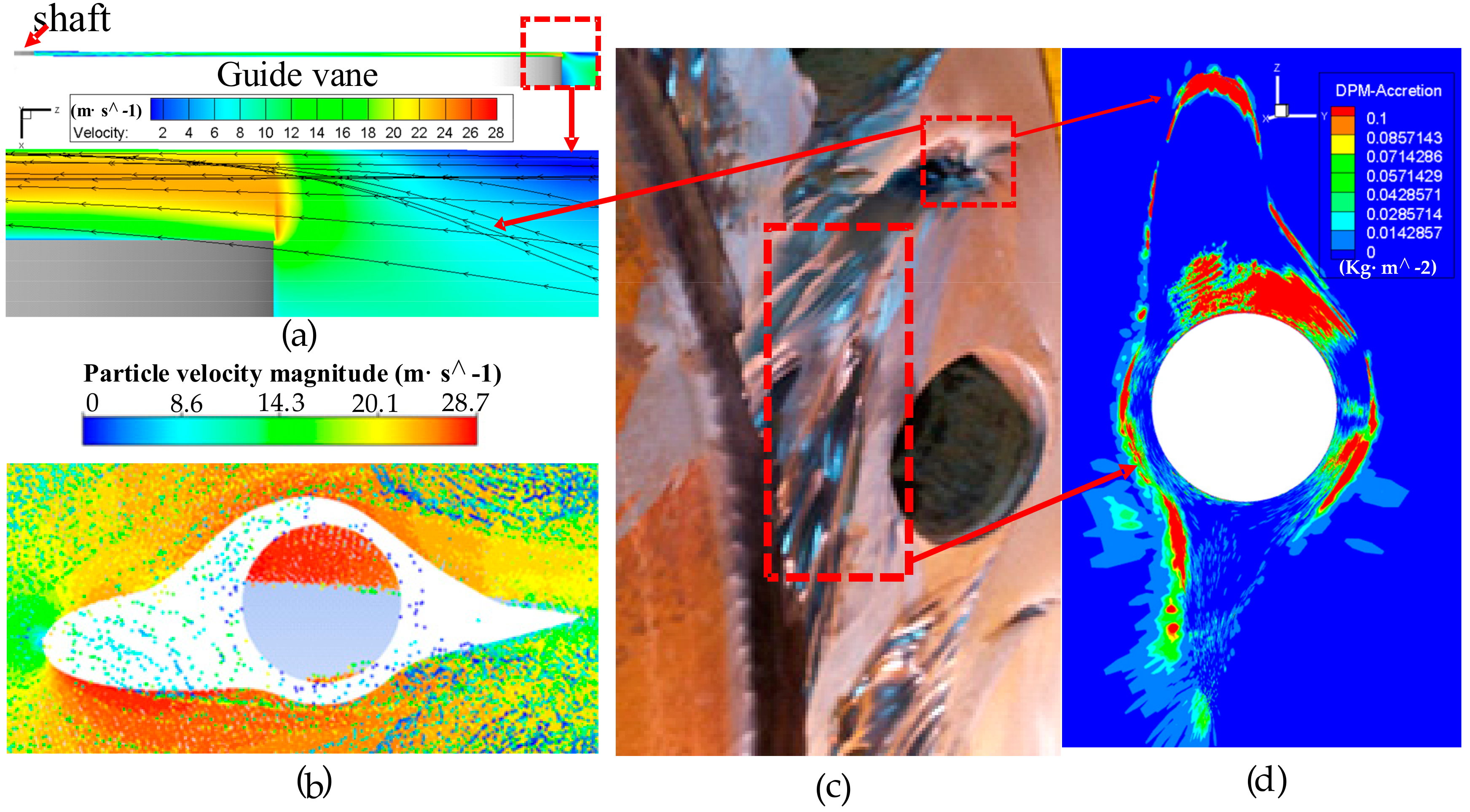
This hydropower station is a run-off hydroelectric station without storage capacity, which fails to discharge sand effectively in service, resulting in a high concentration of sediment. After operation through two flood seasons with a sediment-laden river, no obvious sediment erosion was found when the distributor was under a heavy load. Whereas in the dry season, the sediment erosion of the distributor was very serious. Through the numerical simulation of the three-dimensional flow field of the turbine, the velocity and pressure in the head cover was uniformly distributed, and there was no negative pressure zone and no flow separation. Therefore, under normal circumstances, the hydrodynamic cavitation does not take place in the guide vane, head cover region, and bottom ring. Therefore, sediment erosion is the main reason for the erosion of the distributor flow-passage walls. The sediment erosion regions mostly focus on the guide vane, head cover, bottom ring, upper and lower fixed wearing ring, guide vane sleeve, etc. There were abrasion pits of 5–15 mm on the upper and lower end surfaces behind the guide vane shaft, the erosion depth of the end clearance of guide vane was 10–20 mm, and sediment erosion of the guide vane sleeve was more severe.

Sediment samples from three different positions at the Dongshuixia hydropower station forebay were collected by a suspended sediment sampler. The weight of each sample was not less than 50 g, and the distance between the sampling points was about 12 km. After the clarifying, pouring out the clear water, and drying steps, a laser granularity analyzer was used to analyze the particle size in this study. The median particle size d₅₀ of the sand particles entering the turbine was 45 μm, and its average density was 2650 kg/m³.

3. CFD Predictions

Computational fluid dynamics (CFD) was conducted using the commercially available ANSYS Fluent 19.0, which offers discrete phase models (DPM). This model considers the interactions between particles and fluids. The fluid phase was treated as a continuum by solving the Navier–Stokes equations, while the dispersed phase was solved by tracking a large number of particles through the calculated flow field. The steady simulation results of the SST k-ω turbulence model (number of iterations: 10,000) were used as the initial value of the LES calculation. These models were used to model the turbulent flow due to their superiority for complex turbulence in the clearance.

3.1. Liquid Phase Model

In order to study the relationship between turbulent characteristics and erosion wear in the end-clearance of turbine guide vane in detail, LES model with high precision on turbulence simulation is used to simulate the flow field. The instantaneous motion signals of turbulence were decomposed into two parts: The vortex motion of the large-scale structures and small-scale structures by LES through the filter function. In the process, large vortices were directly calculated, while small vortices were modeled. The filter function G(x, x′) used in the paper can be written as follows:

$$G(\mathrm{x}-{\mathrm{x}}^{\prime })=\left\{\begin{array}{l}1/\Delta \\ 0\end{array}\right.\begin{array}{l}\left|\mathrm{x}-{\mathrm{x}}^{\prime }\right|\le \Delta /2\\ \left|\mathrm{x}-{\mathrm{x}}^{\prime }\right|>\Delta /2\end{array},$$

(1)

where Δ is the mean scale of grid (m); x is the space coordinate on the large-scale space after filtering; and x′ is the space coordinate of the actual flow region.

The governing equations obtained after filtering are:

$$\left.\begin{array}{l}\frac{\partial \left(\rho {\overline{\mathrm{u}}}_{\mathrm{i}}\right)}{\partial t}+\frac{\partial \left(\rho {\overline{\mathrm{u}}}_{\mathrm{i}}{\overline{\mathrm{u}}}_{\mathrm{j}}\right)}{\partial {\mathrm{x}}_{\mathrm{j}}}=-\frac{\partial \overline{p}}{\partial {\mathrm{x}}_{\mathrm{i}}}+\frac{\partial }{\partial {\mathrm{x}}_{\mathrm{j}}}\left[\mu \left(\frac{\partial {\overline{\mathrm{u}}}_{\mathrm{i}}}{\partial {\mathrm{x}}_{\mathrm{j}}}+\frac{\partial {\overline{\mathrm{u}}}_{\mathrm{j}}}{\partial {\mathrm{x}}_{\mathrm{i}}}\right)\right]+\frac{\partial {\tau }_{\mathrm{ij}}}{\partial {\mathrm{x}}_{\mathrm{j}}}\\ \frac{\partial \left(\rho {\overline{\mathrm{u}}}_{\mathrm{i}}\right)}{\partial {\mathrm{x}}_{\mathrm{i}}}=0\end{array}\right\},$$

(2)

where ${\overline{\mathrm{u}}}_{\mathrm{i}}$ and ${\overline{\mathrm{u}}}_{\mathrm{j}}$ are the velocity vectors of the grid scale in the x_i and x_j direction (m/s); $\overline{p}$ is the static pressure of the grid scale (Pa); ρ is the fluid density (kg/m³); μ is the hydrodynamic viscosity (Pa·s); ${\tau }_{\mathrm{i}}{}_{\mathrm{j}}$ is the stress tensor of sub-grid scale (Pa); ${\tau }_{\mathrm{i}}{}_{\mathrm{j}}=-\rho (\overline{{\mathrm{u}}_i{\mathrm{u}}_j}-{\overline{\mathrm{u}}}_{\mathrm{i}}{\overline{\mathrm{u}}}_{\mathrm{j}})$, which shows the influence of small-scale vortex motion on the momentum transportation of a large-scale vortex, and was obtained by the subgrid scale model. The standard Smagorinsky-Lilly model is generally adopted, but the introduced model parameter Cs will affect the turbulence parameter (turbulent dissipation rate). In this study, a dynamic Smagorinsky-Lilly model was adopted, which assumes that the subgrid stress is proportional to the strain rate of the local fluid, and the expression is as follows:

$${\tau }_{ij}=2{\nu }_t\overline{{\mathrm{S}}_{i\mathrm{j}}},$$

(3)

$${\tau }_{ij}=\frac{1}{2}\left(\frac{\partial {\overline{\mathrm{u}}}_{\mathrm{i}}}{\partial {\mathrm{x}}_j}+\frac{\partial {\overline{\mathrm{u}}}_{\mathrm{j}}}{\partial {\mathrm{x}}_i}\right),$$

(4)

$${\nu }_{\mathrm{t}}=L_s^2\left|\overline{S}\right|,$$

(5)

$$\left|\overline{S}\right|=\sqrt{2{\overline{S}}_{\mathrm{ij}}{\overline{S}}_{\mathrm{ij}}},$$

(6)

$$L_{\mathrm{s}}=\min \left(\kappa d,C_s{V}^{1/3}\right),$$

(7)

where $\kappa$ is the von Kármán constant and generally taken as 0.42. In the dynamic Smagorinsky–Lilly model, C_s is not a constant, and needs to be calculated according to the local flow field information to simulate the flow field more accurately.

3.2. Solid Phase Model

The DPM used by ANSYS Fluent contains the assumption that the solid phase is sufficiently dilute so that the particle–particle interactions are negligible. In practice, these issues imply that the discrete phase must be present at a fairly low volume fraction, usually less than 10–12% [20]. In this study, the volume fraction of the sediment particles was calculated as 0.04%, which meets the calculation requirements of DPM model.

The trajectory of a discrete phase particle is determined by integrating the force balance on the particle, which is written in a Lagrangian reference frame. This force balance equates the particle inertia with the forces acting on the particle, and can be written as

$$m_p\frac{d{\overrightarrow{u}}_p}{dt}=m_p\frac{\overrightarrow{u}-{\overrightarrow{u}}_p}{{\tau }_r}+m_p\frac{\overrightarrow{g}\left({\rho }_p-\rho \right)}{{\rho }_p}+\overrightarrow{F},$$

(8)

where $m_p$ is the particle mass (kg); $\overrightarrow{u}$ is the fluid phase velocity (m/s); ${\overrightarrow{u}}_p$ is the particle velocity (m/s); $\rho$ is the fluid density (kg/m³); ${\rho }_p$ is the particle density (kg/m³); $\overrightarrow{F}$ is an additional force (N); $m_p\frac{\overrightarrow{u}-{\overrightarrow{u}}_p}{{\tau }_r}$ is the drag force; and ${\tau }_r$ is the particle relaxation time calculated by:

$${\tau }_r=\frac{{\rho }_p{d}_p^2}{18\mu }\frac{24}{C_d\mathrm{Re}},$$

(9)

where, μ is the molecular viscosity of the fluid (Pa·s); d_p is the particle diameter (mm); C_d is the drag coefficient; and R_e is the relative Reynolds number, which is defined as:

$$\mathrm{Re}\equiv \frac{\rho d_p\left|{\overrightarrow{u}}_p-\overrightarrow{u}\right|}{\mu }.$$

(10)

Equation (8) incorporates additional forces ($\overrightarrow{F}$) in the particle force balance that can be important, which includes the virtual mass, pressure gradient, and Saffman’s lift force. The virtual mass and pressure gradient forces are important when the density ratio of the density of the fluid and the particles is greater than 0.1. The virtual mass force (${\overrightarrow{F}}_{\mathrm{m}}$) required to accelerate the fluid surrounding the particle. The pressure gradient forces (${\overrightarrow{F}}_p$) arise due to the pressure gradient in the fluid. The Saffman’s lift force arises due to shear.

$${\overrightarrow{F}}_{\mathrm{m}}=C_{\nu \mathrm{m}}{m}_p\frac{\rho }{{\rho }_p}\left({\overrightarrow{u}}_p\nabla \overrightarrow{u}-\frac{d{\overrightarrow{u}}_p}{dt}\right),$$

(11)

where $C_{\nu \mathrm{m}}$ is the virtual mass factor with a default value of 0.5.

$${\overrightarrow{F}}_p=m_p\frac{\rho }{{\rho }_p}{\overrightarrow{u}}_p\nabla \overrightarrow{u}.$$

(12)

For non-spherical particles Haider and Levenspiel [21] developed the correlation:

$$C_d=\frac{24}{R{e}_{sph}}\left(1+b_{1}R{e}_{sph}{}^{b_2}\right)+\frac{b_{3}R{e}_{sph}}{b_4+R{e}_{sph}},$$

(13)

where:

$$\begin{gathered} b_1=\exp \left(2.3288-6.4581\phi +2.4486{\phi }^2\right), \\ {b}_2=0.0964+0.5565\phi , \\ {b}_3=\exp \left(4.905-13.8944\phi +18.4222{\phi }^2-10.2599{\phi }^3\right), \\ {b}_4=\exp \left(1.4681+12.2584\phi -20.7322{\phi }^2+15.8855{\phi }^3\right). \end{gathered}$$

The shape factor $\phi$ is defined as:

$$\phi =\frac{s}{S},$$

(14)

where s is the surface area of a sphere having the same volume as the particle, and S is the actual surface area of the particle. The handbook by W.C. Yang [22] indicates the sphericity of sharp and round sand particles to be 0.66 and 0.86, respectively. Therefore, the shape factor is given as 0.86 of round sand particles in this study.

The particle rebound characteristics (velocity and angle) must be calculated to obtain the trajectory of particles after it collides with the flow passage walls. The particle rebound velocity is less than the impingement velocity, which is described by the pertinent restitution ratios. The particle rebound model mainly includes the stochastic particle-wall rebound model by Grant and Tabakoff [23] and the non-stochastic particle-wall rebound model by Forder et al. [24]. In this study, the Tabakoff particle rebound model [25] was adopted. The pertinent restitution ratios are defined as follows:

$${\mathrm{e}}_{\mathrm{N}}\equiv 1.0-0.0211\theta +0.00228{\theta }^2-0.000000876{\theta }^3,$$

(15)

$${\mathrm{e}}_{\mathrm{T}}\equiv 0.953-0.000446\theta +0.00000648{\theta }^3,$$

(16)

where ${\mathrm{e}}_{\mathrm{N}}$ is the normal restitution ratio; ${\mathrm{e}}_{\mathrm{T}}$ is the tangential restitution ratio; and θ is the impingement angle of the particle between the impact trajectory of the particle and the tangential surface across the impact point (°).

3.3. Erosion Model

The choice of the erosion model and correlation coefficients have influence on the erosion wear results, and the research results of Messa G V and Malavasi S are support the above view [26]. In this study, the erosion rate and erosion pattern on the surface of the flow passage components caused by the impacts of sand particles were calculated using the generic erosion model. The erosion rate is defined as:

$$R_{\mathrm{erosion}}={\displaystyle \sum _{p=1}^{N_{\mathrm{particle}s}}\frac{{\dot{m}}_{p}C\left(d_p\right)f(\gamma ){\nu }^{b\left(v\right)}}{A_{face}}},$$

(17)

where $C\left(d_p\right)$ is a function of the particle diameter; $\gamma$ is the impact angle of the particle path with the wall face; $f\left(\gamma \right)$ is a function of impact angle; $\nu$ is the relative particle velocity; $b\left(\nu \right)$ is a function of relative particle velocity; A_face is the area of the cell face at the wall (m²); and ${\dot{m}}_p$ is the mass flow rate of particles impinging on the wall (kg/s).

The Tulsa angle dependent model is used to determine the correlation coefficient, which are suitable for steel being eroded by sand [27]. In this study, the guide vane material specified in the clearance wall is ZGO4Cr13Ni5Mo, which is stainless steel. There are similarities between stainless steel and steel in material properties. Therefore, the selection of the erosion model and correlation coefficients are reasonable, but some error on the erosion magnitude is expected:

$$C({\mathrm{d}}_p)=1.559{\mathrm{e}}^{-6}{B}^{-0.59}\times F_s,$$

(18)

where F_s is a particle shape coefficient as 0.2 for fully rounded sand [27]; B is the Brinell hardness as 309 N/mm² for ZGO4Cr13Ni5Mo of the wall material.

$${\nu }^{b\left(v\right)}={\nu }^{1.73}.$$

(19)

$$f\left(\gamma \right)=\left\{\begin{array}{l}0+22.7\gamma -38.4{\gamma }^2\\ 2+6.8\gamma -7.5{\gamma }^2+2.25{\gamma }^3\end{array}\right.\begin{array}{l}\gamma \le 0.267\mathrm{rad}\\ \gamma \rangle 0.267\mathrm{rad}\end{array}$$

(20)

From formula 17 and 20, when other variables are constant, the erosion rate is the largest with the impact angle as 0.634 rad. When the impact angle is less than 0.634 rad, the erosion rate increases with the increase of the impact angle. When the impact angle is greater than 0.634 rad, the erosion rate decreases with the increase of the impact angle.

The accretion rate is defined as:

$${\mathrm{R}}_{\mathrm{accretion}}\equiv {\displaystyle \sum _{p=1}^{N_{particles}}\frac{{\dot{m}}_p}{A_{face}}}.$$

(21)

3.4. Computational Domain

The guide vane used in turbine (HLA351-LJ-180) is a prototype with a net head of 189 m and capacity of 18.4 MW. A small end-clearance was present to adjust the guide vane angle, depending on the load or flow variation. The structure diagram of the end-clearance between the guide vane and the head cover of the turbine is shown in Figure 4.

The design size of the end-clearance guide vane was 0.22 mm. However, the head cover is raised upward under the high-pressure effect of water in practical operation, making the actual clearance size slightly larger than the designed size, so that it reaches 1 mm. Therefore, the clearance size of 1 mm was used to study the turbulence and sediment erosion characteristics in the end-clearance. To study the influence of a guide vane with a large eccentric shaft on clearance flow (including the flow around the cylindrical shaft) and flow around the airfoil, the geometric structure of the upper part of the guide vane airfoil profiles was used in consideration of the computing resources and computing time. The 3D computational model and relative parameters for the end-clearance of the turbine guide vane are shown in Figure 5.

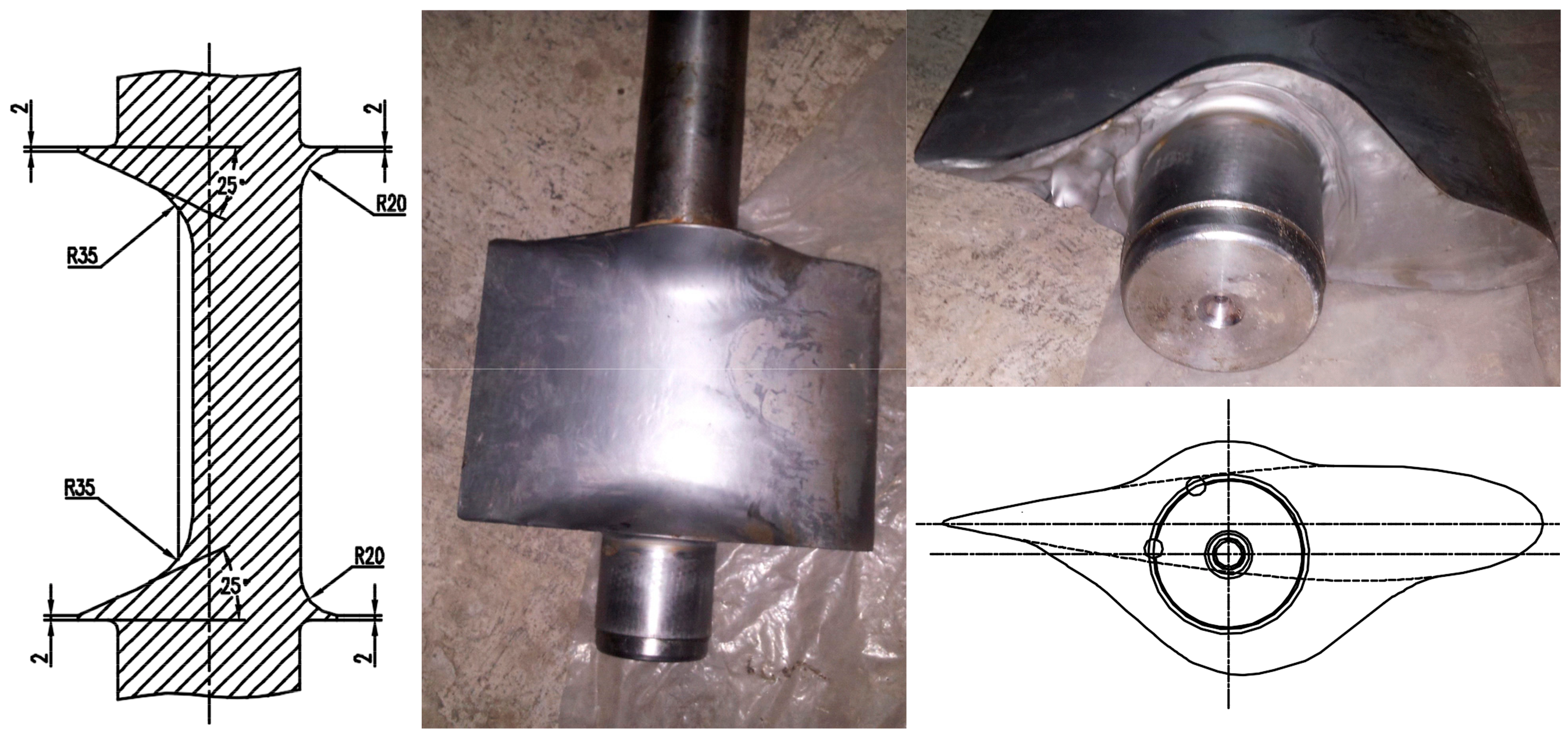
A Francis turbine with a relatively low guide vane height has good watertight condition. However, the end-clearance of a guide vane is rapidly enlarged because of the high-water pressure, large deformation of the head cover, and sediment erosion. Hence, it is of great necessity to solve the leakage of the end-clearance of the guide vane. The guide vane of a Francis turbine used a large eccentric shaft structure (see Figure 6), that is, a large wing plate was added to the upper and lower pressure surface of the guide vane, and the guide vane shaft was enlarged as much as possible. On one hand, this structure increases the retaining water length in the circumferential direction of the guide vane; on the other hand, it increases the covered area of the guide vane end region at the upper and lower facing plate and the leakage resistance. Thus, the leakage of the guide vane end-surface is reduced and the efficiency of the turbine improves. At the same time, this structure can prevent the direct erosion of the guide vane shaft by a sediment-laden river.

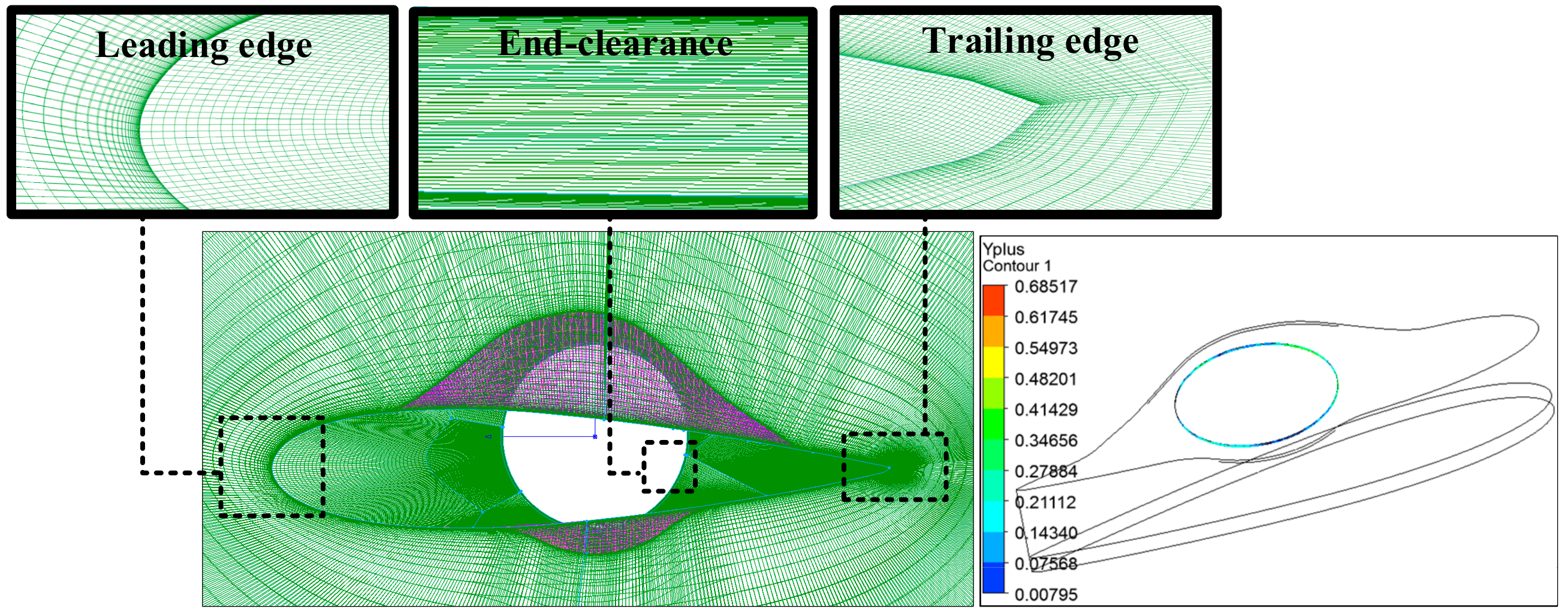
The computational domain was discretized using a structured grid as shown in Figure 7. Boundary layers were utilized to keep y+ within its accepted limits and accurately consider the wall effects. The first layer thickness of 0.001 mm in the clearance domain was determined to meet the accuracy of the large eddy simulation calculation of the clearance flow field. Then, the y+ values were controlled to be below 1 in the clearance domain. There were 51 grid layers in the clearance of 1 mm to accurately capture the turbulence characteristics. For the purpose of confirming that the grid pattern used was adequate, a grid convergence test was conducted on five different grid numbers. With the increase of grid numbers, the variable quantity of pressure drops between inlet1 and outlet1 is less than 2% as the test standard. Finally, the grid numbers in the computational domain was 7.143 million.

3.5. Numerical Setup

To achieve an improved convergence, the finite volume method and SIMPLEC algorithm were utilized to disperse and compute the flow controlling equations. The first order upwind discretization scheme was used for both the convection and divergence terms. In the unsteady calculation (LES), the total calculation time was set as 1 s. Among the time steps, the size was defined as 0.0001 s, and the number of time steps was 10,000. The above calculations include the gravity effect. To obtain a converged solution, the following under relaxation factors were used: 0.3 for pressure, 1 for density, 0.35 for momentum, and 0.9 for the discrete phase sources. The convergence criteria were set as 1 × 10⁻⁸. The DPM iteration interval was set as 20. When the particles pass through the turbulent vortex, there will be an accompanying motion, which will lead to the lateral diffusion effect of the particles. Therefore, the discrete random walk model (DRW) was used to consider the interaction between the particles and discrete vortices of fluid.

According to the actual conditions and numerical simulation of the whole flow field of a hydro turbine, the fluid through the stay vane enters the end-clearance of the guide vane at a certain angle (under different guide vane openings). Therefore, the “velocity-inlet” boundary condition was used for clearance inlet1 and inlet2, and the velocity of the solid phase was set as the same velocity as that of the fluid phase. The direction of axes X, Y, and Z are shown in Figure 5, the coordinate origin is on the axis, the X-axis is along the axis and the Z-axis and the Y-axis are parallel and perpendicular to the chord length of the guide vane airfoil, respectively. The Y-velocity was −0.69799 m/s, and the Z-velocity was −19.9878 m/s. The “pressure-outlet” boundary condition at the outlet was set with the pressure of 1,300,000 pa, and nonslip flow conditions were used for the walls. Except the clearance inlet and outlet, the “wall” boundary condition was used for other surfaces. The roughness constant was set at a value of 0.5. Trajectories of the sediment particles were tracked by the Lagrangian method. At the inlet and outlet of the clearance flow, the boundary conditions for the solid phase were set as “escape” and the rest of the walls were set as “reflect”. The guide vane material specified in the clearance wall is ZGO₄Cr₁₃Ni₅Mo with a density of 7790 kg/m³. The density and viscosity of the clear water phase was assumed to be 998.2 kg/m³ and 0.001003 kg/(m·s), respectively. Furthermore, the sediment particles were assumed to be uniform and round shaped. The Taolai River is neutral water and its mean annual sediment content, average sediment concentration, and maximum sediment concentration was 1.12 kg/m³, 2.5 kg/m³, and 126 kg/m³, respectively. The mean annual sediment content was used as the setting standard for sediment particle concentration. The d₅₀ of the sediment particles was 45 μm and the average density was 2650 kg/m³.

3.6. Independence Test of the Particle Trajectory Number

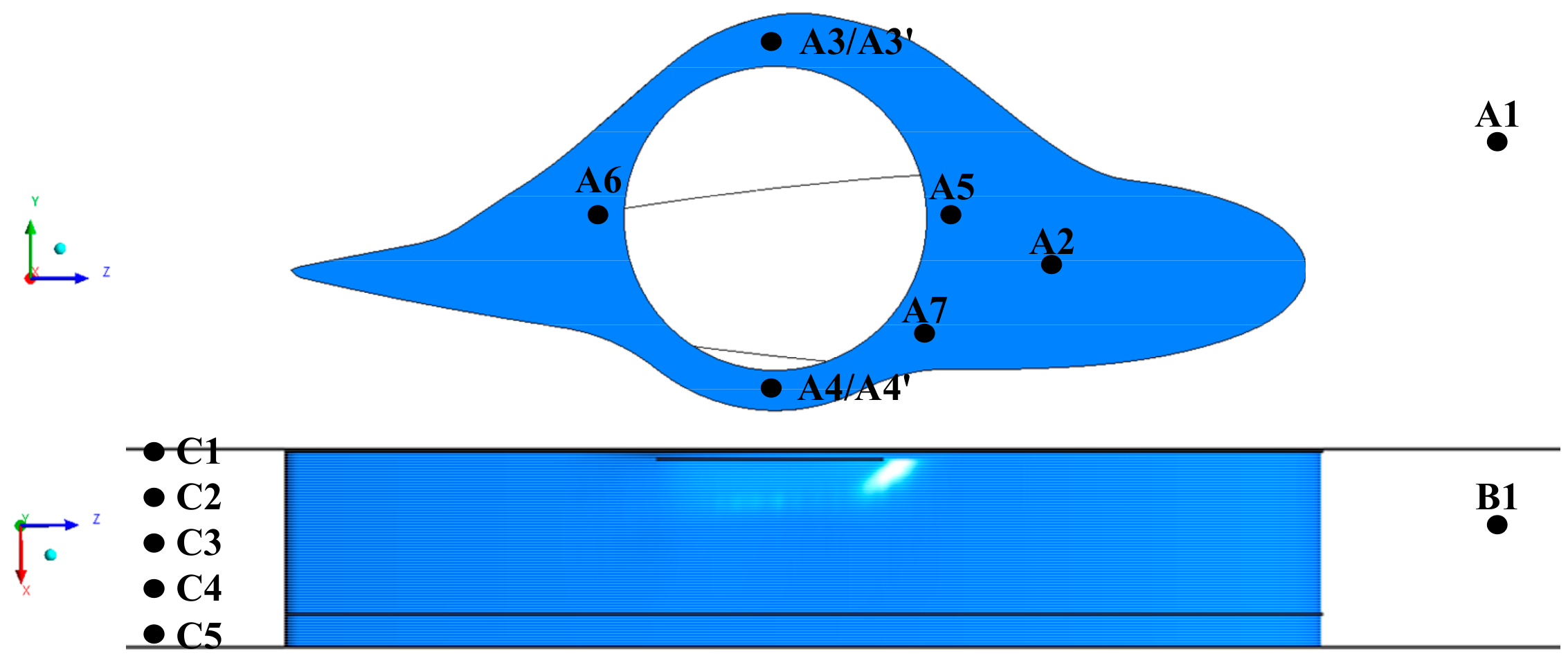
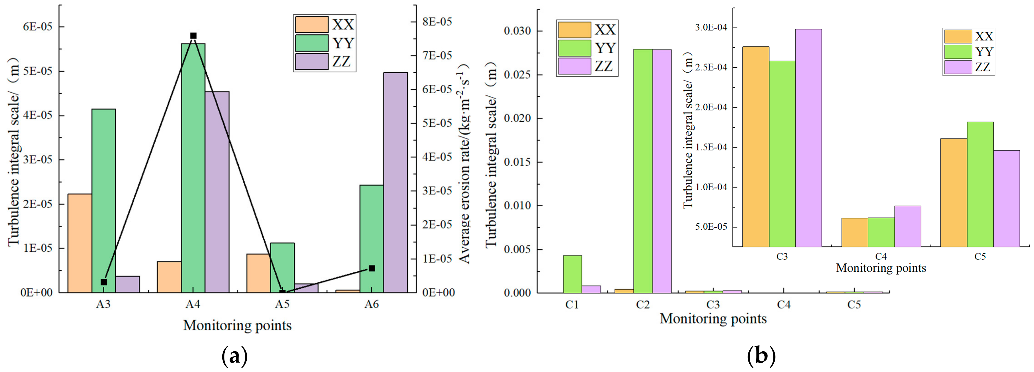
Figure 8 shows the arrangement of the monitoring points. A2–A7 were set at the clearance flow (X = 0.5 mm), and A3–A6 were symmetric along the shaft center. A3′ and A4′ were set at the clearance wall (X = 0 mm). A1 and B1 were set at the inflow, A1 was set at the front of clearance flow, and B1 was set at the front of the guide vane. C1–C5 were isometrically set at the X direction of the guide vane wake.

The interaction between the liquid and solid particle was considered in this paper. The number of particle trajectory per unit inlet area determines the distribution of particles in the horizontal and vertical direction along the inflow, which is very important in the study of the erosion characteristics of the end-clearance surfaces. The total number of injected particles is determined by the total flow rate, which is the product of the inlet section area and average annual sediment concentration. When the total mass flow rate of particles is constant, the number of particle trajectory can be set by setting the sample density in the horizontal and vertical directions. The ratio of the total number of particle trajectory to the area of incident plane is the number of particle trajectory per unit inlet area. A3′ and A4′ are located at the large and small wing surface of the guide vane with erosion wear, which have certain representativeness. Therefore, A3′ and A4′ were selected for the independence test of the particle trajectory number. Numerical simulation of the end-clearance flow of guide vane was conducted with different numbers of particle trajectory per unit inlet area, and the changing rule of the average erosion rate at the monitoring points (A3′ and A4′) was obtained, as shown in Figure 9. The number of particle trajectory per unit inlet area is the abscissa, and the average erosion rate with different ranges are the left and right side vertical coordinate.

With the increase in the number of particle trajectory per unit inlet area (mm²), the average erosion rate increases. When the number of particle trajectory per unit inlet area is greater than 1, the average erosion rate is basically stable. Therefore, in order to ensure converged results for a flow field with a 1 mm clearance, the number of trajectories per unit inlet area should be about 1/mm².

4. Results and Discussion

4.1. Sediment Erosion Mechanism Analysis in End-Clearance Walls of the Guide Vane

Figure 10 shows a comparison of the wear morphology and flow field on the end-surface guide vane. Figure 10a shows the instantaneous velocity field at 1 s of the numerical simulation. It can be seen in Figure 10a that the sand-laden water flowed through the guide vane at a certain angle. The fluid pressure increased before entering the clearance due to the barriers of the airfoil wall and the head cover wall. Next, a pressure difference was produced on the internal and external clearance. The above situation led to an obvious increased velocity of entry into the clearance. The fluid velocity decreased gradually with the further development of the fluid. Additionally, the flow field at the front of the guide vane shaft was uniform without an obvious vortex structure.

Combining Figure 10b–d, it was found that there was basically no accretion of sediment particles and no obvious erosion wear on the end-surface of guide vane before the shaft, which was basically consistent with the actual wear morphology. When the fluid flowed through the shaft, obvious vortex structures appeared on both sides of the shaft due to the disc shear effect. After fluid flowed through the shaft, a symmetrical von Kármán vortex street was observed. Again, by combining Figure 10b–d, it was found that there was a high impact quantity of particles at regions where the vortex appeared, which is mainly because the particles had the following behaviors and will be involved in the vortex. Additionally, the erosion wear was serious in regions where large accretion of particles was observed, which mainly appeared behind the shaft and at both end-surfaces of the shaft. The wear pattern was mainly furrow shaped. On the end-surface after the guide vane shaft, the fluid flowed evenly, so only a few particles impacted, and the erosion wear was small. The above situation was mainly because the guide vane adopted a large eccentric shaft structure, and the fluid entered the clearance from one side of the large wing surface without being affected by the shaft.

Figure 11 shows a comparison of the wear morphology and flow field on the end-surface of the head cover. As can be seen from Figure 11c, the erosion wear regions on the end-surface of the head cover mainly focused on the corresponding head cover to the leading edge and the suction side (small wing surface) of the guide vane. On the corresponding head cover to the leading edge of the guide vane, the wear morphology was obviously pit superimposed by multiple erosion. From Figure 11a,b,d, this is because the fluid entered the clearance in an oblique uprush status, the sand particles continuously impacted on the end-surface of the head cover, and the accretion rate and velocity of sand particles were higher here. It can be seen from the above that high velocity, high concentration, and a large impingement angle of sand particles are the main reasons for serious erosion wear. On the corresponding head cover to the suction side of the guide vane, the wear pattern was furrow shaped. However, there was less erosion wear on the corresponding head cover to the pressure side (large wing surface) of the guide vane. This is because the accumulation area and velocity of sand particles on the former were larger than those on the latter. It can also be seen that although the DPM accretion rate of sand particles was larger before the shaft, there was almost no wear from the actual wear morphology. Combined with Figure 11a,b of the instantaneous velocity field and particle velocity field at 1 s of the numerical simulation, the fluid velocity gradually decreased and the velocity defect increased when fluid entered into the clearance to the front of the shaft. The particles had good following performance, the velocity of flow field decreased, and the particle velocity also decreased. Thus, particles with a lower velocity produced less erosion.

The 62 monitoring points were set along the pressure side and suction side of the guide blade of the clearance mid-span to measure the velocity and pressure. Figure 12 shows time-averages of velocity and pressure within 1 s of numerical simulation. Figure 12a,b shows the pressure and velocity distribution along the clearance mid-span, respectively. The x-coordinate is the distance from the leading edge of the guide vane airfoil along the z-direction, and the y-coordinate is the average pressure and average velocity of the monitoring points. Figure 12a shows that the highest pressure at the leading edge of the guide vane was the stagnation point. After the stagnation point, the fluid velocity increased with the decrease in pressure, which is the acceleration phenomenon in the clearance. From the leading edge to 30% of the guide vane chord, the pressure on the pressure side was almost equal, while the pressure on the suction side showed a linearly declining trend, which was in accordance with the pressure distribution law on the airfoil surface under a small attack angle. This indicates that the flow around the airfoil has an influence on the clearance, so that the pressure characteristics of the airfoil surface developed around the clearance. Combining Figure 10a and Figure 11, the flow around the airfoil affected the deflection of the wake behind the clearance shaft. As a result, the small wing surface of the guide vane and the corresponding head cover showed serious erosion. Due to the above pressure characteristics, the modification of the airfoil of end-surface can further affect the deflection angle of wake behind the cylindrical shaft, thus reducing the erosion wear behind the shaft. Between 30% and 70% of the guide vane chord, the end surface of the guide blade airfoil was an asymmetric structure protruding from the middle section, and also had the effect of flow around the cylinder shaft. Therefore, the velocity and pressure on the pressure side and suction side had a serious fluctuation in the middle section, pressure difference decreased, and the velocity also decreased sharply. After 70% of the guide vane chord, the pressure difference gradually increased, and the pressure on the pressure side changed to steady after first increasin.

The two XY planes were intercepted to observe the characteristics of leakage flow through the end-clearance of the guide vane at the wake. Figure 13 shows instantaneous velocity field at 1 s of numerical simulation. It can be seen from Figure 13 that the leakage vortex not only appeared at the trailing edge of the airfoil, but also appeared at the large and small wing surfaces of both sides of the shaft. This was mainly because the large eccentric shaft prevented the fluid from flowing smoothly through the shaft, so that part of the fluid flowed out directly at the large and small wing surfaces to form leakage vortices. In addition, the fluid tended to flow along the position of the X positive axis with the leakage vortices developing downstream, which may lead to serious erosion wear in the downstream part of the runner inlet behind the guide vane.

4.2. Turbulence Characteristics in the End-Clearance of the Guide Vane

The turbulence integral scales of each monitoring point in three directions were calculated by the direct integration of the autocorrelation function. The turbulence integral scale of different monitoring points is shown in Figure 14. The turbulence integral scale of each monitoring point in the X direction was small and the variable quantity was not large, which was mainly caused by the limitation of the clearance size. Meanwhile, the significant turbulence integral scale changes in the Y and Z direction were mainly due to a lack of restriction on the clearance size. By comparing the wear morphology in Figure 10 and Figure 11, the turbulence integral scale in the Y and Z direction was large where the erosion regions were larger. The turbulence integral scale was larger, which showed that the vortex was larger. Then, more sand particles rolled up to the rotational motion by vortex, given that rotational motion makes sand particles have enough velocity and impingement angle to damage the flow-passage surfaces. That is, a larger turbulence integral scale makes a larger wear region, which was verified by the large and small wing surface wear. By comparing Figure 14a with Figure 13, the turbulence integral scale increased sharply at the Y and Z direction of C2. This was mainly affected by two factors: (1) The leakage vortex flowed down and only went through C2, and (2) the turbulence scale of the wake was larger at C2 due to the guide vane with a large eccentric shaft. A sediment-laden vortex with a large turbulence scale will cause serious wear of the runner inlet.

To analyze the turbulent flow characteristics of monitoring points, turbulent kinetic energy (TKE) and coherent turbulence kinetic energy (CTKE) are defined, which is given as:

$$TKE(\mathrm{t})=\frac{1}{2}\left[u_{\mathrm{x}}\prime {\left(t\right)}^2+u_{\mathrm{y}}\prime {\left(t\right)}^2+u_z\prime {\left(t\right)}^2\right],$$

(22)

where $u_x\prime \left(t\right)$, $u_y\prime \left(t\right)$, and $u_z\prime \left(t\right)$ are the fluctuation values of axial velocity, lateral velocity, and vertical velocity, respectively.

$$CTKE(\mathrm{t})=\frac{1}{2}{\left[{\left(u_x\prime \left(t\right)u_y\prime \left(t\right)\right)}^2+{\left(u_x\prime \left(t\right)u_z\prime \left(t\right)\right)}^2+{\left(u_y\prime \left(t\right)u_z\prime \left(t\right)\right)}^2\right]}^{1/2}.$$

(23)

The horizontal flow angle $\psi \prime (\mathrm{t})$ and the vertical flow angle $\alpha \prime (\mathrm{t})$ of the velocity fluctuation can be calculated with Equations (4) and (5). Thus, the direction variant characteristics of turbulent fluctuation at monitoring points can be obtained:

$$\psi \prime (\mathrm{t})={\tan }^{-1}\left(u_y\prime \left(t\right)/u_z\prime \left(t\right)\right).$$

(24)

$$\alpha \prime (\mathrm{t})={\tan }^{-1}\left(u_x\prime \left(t\right)/u_z\prime \left(t\right)\right).$$

(25)

The TKE and CTKE of the monitoring points are shown in Figure 15. From Figure 15a, the TKE and CTKE in the clearance were greater than that outside the clearance. Combining Figure 10, Figure 12, and Figure 14, the TKE and CTKE of A5 was greater than A4, but there was almost no erosion at A5. This is because the pressure drop was obvious, the flow field was evenly distributed, the turbulence integral scale was small, and the particles were not deposited at A5. In addition, the wear region size and erosion rate of the wing surface of A4 were larger than that of A3, but the TKE and CTKE at A4 were smaller. The above results explain that TKE and CTKE were not a determinant for sediment wear. According to the calculations through Equations (24) and (25), the horizontal and vertical flow angles of A4 were 42.49° and 11.62°, respectively, which were larger than the 10.64° and 22.53° of A3, and the turbulence integral scale of A4 was also larger than A3, which further indicates that erosion wear was closely related to the turbulence integral scale and turbulence angle. Figure 15b shows that the TKE and CTKE at C2 were greater than that at the other points at the guide vane wake. Combined with Figure 14b, the turbulence integral scales, TKE and CTKE, at C2 were both large. The characteristics of leakage vortex and wake at the large wing surface were obvious at C2, which would cause greater erosion wear on the runner inlet.

To study the spectrum characteristics of turbulent flow in the clearance, a power spectrum analysis was carried out on the pulsation velocity of the three directions of A3, A4, A5, and A6, as shown in Figure 16. From Figure 16a, the trend from low frequency to high frequency in the three directions of A3 was the same as A4, which is mainly because A3 and A4 were located at both sides of the shaft and the flow at both sides had similarity. However, except for the low frequency part in the Y direction, A3 in all directions and frequencies contained much more energy than A4, which verified the conclusion in Figure 15. A3 and A4 had the highest energy in the Z direction, followed by the Y direction, and the lowest energy in the X direction. From Figure 16b, in the X direction, the energy of A5 at the front of the shaft was greater than A6 at the back of the axis, which explains that the energy in the X direction decreased after the fluid flowed through the shaft. In the Y direction, the energy of A6 between 4 Hz and 40 Hz was greater than A5, while that of the other frequencies was less than A5. In the Z direction, A6 contained more energy in the low frequency than A5, while the high frequency was less than A5. In the above, the TKE, CTKE, and erosion rate of A6 were all greater than A5, which explains that the energy in the low frequency plays a leading role in turbulent kinetic energy, and high frequency small-scale turbulence has little influence on the erosion wear. For this conclusion, the roughness on the surface of the shaft can be increased to the separation delay of the cylinder shaft surface, reduce the wake area, and reduce the low-frequency energy, so as to reduce erosion.

5. Conclusions

Erosion wear in the end-clearance of the turbine guide vane is a critical problem for hydropower stations, which must be investigated to reduce erosion damage and improve the operating efficiency of the turbine. In this study, the end-clearance flow of a guide vane with a large eccentric shaft was used as the research object, and numerical calculations with LES and DPM models were carried out to study the sediment erosion characteristics and mechanism in the guide vane end-clearance of a Francis turbine. The following can be concluded from this study:

(a)

For a flow field with a 1 mm clearance, the number of particle trajectory per unit inlet area should be about 1, based on an independence test of the particle trajectory number.

(b)

The flow field at the front of the guide vane shaft was evenly distributed, and there was no obvious vortex structure, so there was basically no erosion wear. However, obvious vortex structures appeared on both sides of the shaft due to the disc shear effect. After fluid flowed through the shaft, the symmetrical von Kármán vortex street was observed. Thus, regions where the vortex occurred had obvious erosion wear. When the turbulence integral scale, turbulent angle, and TKE all increase, this will lead to the more serious wear condition.

(c)

The flow around the airfoil has an influence on the clearance, so that the pressure characteristics of the airfoil surface develops around the clearance. Then, it affects the flow direction of the wake behind the clearance shaft. As a result, the small wing surface of the guide vane and the corresponding head cover showed serious erosion.

(d)

The energy in the low frequency plays a leading role in turbulent kinetic energy, and high frequency small-scale turbulence has little influence on the erosion wear.

References

1. Ma, Y.T.; Xing, Y.L. The situation and prospect of hydropower in China. Energy Eng. 2003, 4, 1–4. [Google Scholar]
2. Neopane, H.P. Sediment Erosion in Hydro Turbines. Ph.D. Thesis, Norwegian University of Science and Technology, Trondheim, Norway, 2010. [Google Scholar]
3. Thapa, B.S.; Dahlhaug, O.G.; Thapa, B. Sediment erosion in hydro turbines and its effect on the flow around guide vanes of Francis turbine. Renew. Sustain. Energy Rev. 2015, 49, 1100–1113. [Google Scholar] [CrossRef]
4. Nicolet, C.; Ruchonnet, N.; Avellan, F. One-dimensional modeling of rotor stator interaction in Francis pump-turbine. In Proceedings of the 23rd IAHR Symposium on Hydraulic Machinery and Systems, Yokohama, Japan, 17–21 October 2006. [Google Scholar]
5. Chen, X. Theoretical and Experimental Study of Flow Through the Double Cascade of a FRANCIS Turbine. Ph.D. Thesis, Norwegian University of Science and Technology, Trondheim, Norway, 1992. [Google Scholar]
6. Thapa, B.S.; Dahlhaug, O.G.; Thapa, B. Velocity and pressure measurements in guide vane clearance gap of a low specific speed Francis turbine. IOP Conf. Ser. Earth Environ. Sci. 2016, 49, 062019. [Google Scholar] [CrossRef] [Green Version]
7. Thapa, B.S.; Dahlhaug, O.G.; Thapa, B. Effects of sediment erosion in guide vanes of Francis turbine. Wear 2017, 390–391, 104–112. [Google Scholar] [CrossRef]
8. Thapa, B.S.; Dahlhaug, O.G.; Thapa, B. Sediment erosion induced leakage flow from guide vane clearance gap in a low specific speed Francis turbine. Renew. Energy 2017, 107, 253–261. [Google Scholar] [CrossRef]
9. Koirala, R.; Zhu, B.S.; Neopane, H.P. Effect of Guide Vane Clearance Gap on Francis Turbine Performance. Energies 2016, 9, 275. [Google Scholar] [CrossRef]
10. Tallman, J.; Lakshminarayana, B. Numerical simulation of tip leakage flows in axial flow turbines, with emphasis on flow physics: Part I- Effect of tip clearance height. J. Turbomach. 2001, 123, 314–323. [Google Scholar] [CrossRef]
11. Noon, A.A.; Kim, M.H. Erosion wear on Francis turbine components due to sediment flow. Wear 2017, 378–379, 126–135. [Google Scholar] [CrossRef]
12. Messa, G.V.; Mandelli, S.; Malavasi, S. Hydro-abrasive erosion in Pelton turbine injectors: A numerical study. Renew. Energy 2019, 130, 474–488. [Google Scholar] [CrossRef]
13. Leguizamon, S.; Jahanbakhsh, E.; Alimirzazadeh, S.; Maertens, A.; Avellan, F. Multiscale simulation of the hydroabrasive erosion of a Pelton bucket: Bridging scales to improve the accuracy. Int. J. Turbomach. Propuls. Power 2019, 4, 9. [Google Scholar] [CrossRef]
14. Leguizamón, S.; Jahanbakhsh, E.; Maertens, A.; Alimirzazadeh, S.; Avellan, F. Simulation of the hydroabrasive erosion of a bucket: A multiscale model with projective integration to circumvent the spatio-temporal scale separation. IOP Conf. Ser. Earth Environ. Sci. 2019, 240, 072014. [Google Scholar] [CrossRef]
15. Brekke, H. Design of hydraulic machinery working in sand laden water. In Abrasive Erosion and Corrosion of Hydraulic Machinery, 1st ed.; Duan, C.G., Karelin, V.Y., Eds.; Imperial College Press: London, UK, 2002; pp. 155–181. [Google Scholar]
16. Koirala, R.; Thapa, B.; Neopane, H.P.; Zhu, B. Sediment erosion in guide vanes of Francis turbine: A case study of Kaligandaki Hydropower Plant, Nepal. Wear 2016, 362–363, 53–60. [Google Scholar] [CrossRef]
17. Han, W.; Kang, J.B.; Wang, J. Erosion estimation of guide vane end clearance in hydraulic turbines with sediment water flow. Mod. Phys. Lett. B 2018, 32, 1850100. [Google Scholar] [CrossRef]
18. Han, W.; Chen, Y.; Li, R.N. Sediment-wear morphology prediction method of hydraulic machine based on differential-quadrature method. Mod. Phys. Lett. B 2019, 33, 1950172. [Google Scholar] [CrossRef]
19. Han, W.; Chen, Y.; Liu, Y.; Wei, S.Z. Prediction of erosional shape evolution in end-surface clearance of turbine guide vane. Trans. Chin. Soc. Agric. Eng. 2018, 34, 100–107. [Google Scholar]
20. ANSYS, Inc. Limitation on the Particle Volume Fraction. ANSYS 19.0 Help; ANSYS, Inc.: Canonsburg, PA, USA, 2018. [Google Scholar]
21. Haider, A.; Levenspiel, O. Drag Coefficient and Terminal Velocity of Spherical and Nonspherical Particles. Powder Technol. 1989, 58, 63–70. [Google Scholar] [CrossRef]
22. Yang, W.C. Handbook of Fluidization and Fluid-Particle Systems; Marcel Dekker Inc.: New York, NY, USA, 2003. [Google Scholar]
23. Grant, G.; Tabakoff, W. Erosion Prediction in Turbomachinery Resulting from Environmental Solid Particles. J. Aircr. 1975, 12, 471–478. [Google Scholar] [CrossRef]
24. Forder, A.; Thew, M.; Harrison, D. A numerical investigation of solid particle erosion experienced within oilfield control valves. Wear 1998, 216, 184–193. [Google Scholar] [CrossRef]
25. Wakeman, T.; Tabakoff, W. Measured Particle Rebound Characteristics Useful for Erosion Prediction. In Proceedings of the ASME 1982 International Gas Turbine Conference and Exhibit, London, UK, 18–22 April 1982. [Google Scholar]
26. Messa, G.V.; Malavasi, S. The effect of sub-models and parameterizations in the simulation of abrasive jet impingement tests. Wear 2017, 370–371, 59–72. [Google Scholar] [CrossRef]
27. Edwards, J.K.; McLaury, B.S.; Shirazi, S.A. Supplementing a CFD Code with Erosion Prediction Capabilities. In Proceedings of the ASME FEDSM’98, ASME 1998 Fluids Engineering Division Summer Meeting, Washington, DC, USA, 21–25 June 1998. [Google Scholar]
Figure 1. Sediment erosion in the flow passage components of the turbine: (a) Guide vane; (b) runner; and (c) hydropower station in a sand-laden river.
Applsci 09 04137 g001
Figure 2. Schematic diagram of end-clearance of the guide vane.
Applsci 09 04137 g002
Figure 3. Dongshuixia hydropower station.
Applsci 09 04137 g003
Figure 4. Schematic diagram in the end-clearance of a turbine guide vane.
Applsci 09 04137 g004
Figure 5. Computational model and relative parameters (mm).
Applsci 09 04137 g005
Figure 6. Guide vane with a large eccentric shaft.
Applsci 09 04137 g006
Figure 7. Computational grid and y+ values for the clearance flow domain.
Applsci 09 04137 g007
Figure 8. Arrangement of the monitoring points.
Applsci 09 04137 g008
Figure 9. Independence test of the particle trajectory number.
Applsci 09 04137 g009
Figure 10. Comparison of wear morphology and flow field on the end-surface of the guide vane: (a) Flow field; (b) discrete phase model (DPM) accretion; (c) DPM erosion; and (d) wear morphology.
Applsci 09 04137 g010
Figure 11. Comparison of wear morphology and flow field on the end-surface of the head cover: (a) Flow field at the leading edge of guide vane airfoil (XZ section); (b) particle velocity in the clearance; (c) wear morphology; and (d) DPM accretion.
Applsci 09 04137 g011
Figure 12. Velocity and pressure measurements along the clearance mid-span: (a) Pressure; and (b) velocity.
Applsci 09 04137 g012
Figure 13. Leakage flow.
Applsci 09 04137 g013
Figure 14. Turbulence integral scale: (a) Turbulence integral scale and average erosion rate of A3–A6; and (b) C1–C5.
Applsci 09 04137 g014
Figure 15. Turbulent kinetic energy (TKE) and coherent turbulence kinetic energy (CTKE): (a) A1–A7; and (b) C1–C5.
Applsci 09 04137 g015
Figure 16. Power spectrum of fluctuating velocity in three directions: (a) A3 and A4 (ux’, uy’, and uz’); and (b) A5 and A6 (ux’, uy’, and uz’).
Applsci 09 04137 g016aApplsci 09 04137 g016b