Article

Multiple Feature Integration for Classification of Thoracic Disease in Chest Radiography

by
Thi Kieu Khanh Ho
1 and
Jeonghwan Gwak
2,*
1
School of Electrical Engineering and Computer Science, Gwangju Institute of Science and Technology, Gwangju 61005, Korea
2
Department of Software, Korea National University of Transportation, Chungju 27469, Korea
*
Author to whom correspondence should be addressed.
Appl. Sci. 2019, 9(19), 4130; https://doi.org/10.3390/app9194130
Submission received: 6 September 2019 / Revised: 24 September 2019 / Accepted: 27 September 2019 / Published: 2 October 2019
(This article belongs to the Special Issue Image Processing Techniques for Biomedical Applications)

Abstract

:

Featured Application

We present handcrafted and deep feature integration approaches to tackle the unified weakly-supervised 14-label chest X-ray image classification and pathological localization.

Abstract

The accurate localization and classification of lung abnormalities from radiological images are important for clinical diagnosis and treatment strategies. However, multilabel classification, wherein medical images are interpreted to point out multiple existing or suspected pathologies, presents practical constraints. Building a highly precise classification model typically requires a huge number of images manually annotated with labels and finding masks that are expensive to acquire in practice. To address this intrinsically weakly supervised learning problem, we present the integration of different features extracted from shallow handcrafted techniques and a pretrained deep CNN model. The model consists of two main approaches: a localization approach that concentrates adaptively on the pathologically abnormal regions utilizing pretrained DenseNet-121 and a classification approach that integrates four types of local and deep features extracted respectively from SIFT, GIST, LBP, and HOG, and convolutional CNN features. We demonstrate that our approaches efficiently leverage interdependencies among target annotations and establish the state of the art classification results of 14 thoracic diseases in comparison with current reference baselines on the publicly available ChestX-ray14 dataset.

1. Introduction

Lung diseases are the leading health-related cause of death worldwide. There is a vital need for screening, early detection, and personalized therapies of lung cancer due to the possibility of contracting it from simple thorax illnesses. Historically, chronic obstructive pulmonary disease, emphysema, chronic bronchitis, and pneumonia have been the major causes of lung cancer [1]. Pneumonia affects approximately 450 million people, resulting in 4 million deaths per year [2]. Because it is low-cost and easily accessible, chest radiography, colloquially called chest X-ray (CXR), has become a common technique, making up nearly 45% of all radiological studies, including the diagnosis of a wealth of pathologies. An enormous number of chest radiological images have been produced globally, which are currently being analyzed through visual examinations on a slice-by-slice basis. Meanwhile, each X-ray scan can comprise dozens of patterns corresponding to hundreds of potential lung diseases, resulting in difficulty of interpretation, a high disagreement rate between radiologists, and unnecessary follow-up procedures. To deal with such a large number of data, a high degree of expertise and concentration are required, which is time-consuming, expensive, and prone to human errors [3]. Therefore, it is important to develop adaptive algorithms for the computer-aided diagnosis (CAD) of thoracic diseases.
Owing to the complexity and diversity of thorax diseases and the limited quality of CXR images, the capability of CAD is limited in the two following steps; the detection of abnormalities and their classification. In general, manual marking of pathologically abnormal regions by an expert requires even more work than labeling them. Thus, chest radiography datasets (e.g., ChestX-ray8 and ChestX-ray14 [4]) have been published, which present disease labels along with a small subset of region-level annotation of abnormal regions [4]; this annotation technique leads to the so-called weakly supervised problem during CAD. As reported in [5], the bounding boxes for localization tasks are much more informative than a single disease class label and significantly improve the model performance. Nevertheless, obtaining detailed disease localization annotations can be expensive and difficult. Therefore, designing models that are effective with a small number of annotated masks is a crucial step for the success of clinical applications. Recently, several attention-based models have been developed and proven to enhance the localization and recognition of multiple objects, despite being given only class labels during the training process [6]. Therefore, such attention mechanism can be used to address the problem of poor localization and recognition of objects in our study.
In the era of computer vision, deep learning-based methods have gained state-of-the-art performances in a variety of domains, including image classification [7,8], scene recognition [9], face recognition [10], and object detection [11]. In addition, the rapid progress of deep learning algorithms has facilitated the establishment of various annotated image datasets [12,13,14,15]. These annotations indicate different characteristics important for the definition of the forthcoming challenges and subsequently possible progress. Yielding similar results in medical image analysis domains (such as human anatomical and pathological structures in radiology imaging), deep learning approaches have led to many works, including in lymph node and interstitial lung disease detection and classification [16,17], pulmonary nodule detection in CT images [18], cerebral micro-bleed detection [19], prediction of spinal radiological scores [20], skin cancer classification [21], and automated pancreas segmentation [22]. Convolutional neural networks (CNNs), one of the most common deep learning techniques, can learn object features in an end-to-end manner considering millions of parameters in the abovementioned studies. However, CNNs require a large number of training images to avoid overfitting issues, and it is still unclear how well deep learning-based techniques can scale up to thousands of patients because previous studies were evaluated on the small-to-middle scale of several hundred patients.
Intuitively, the features are the predominant factor in image representation basis. An image can be seen as a bunch of local patches regardless of the spatial information, which can easily be obtained by clustering shallow handcrafted features such as scale invariant feature transform (SIFT) [23], local binary patterns (LBPs) [24], and histogram of oriented gradients (HOG) [25]. Extracting multiple shallow handcrafted features and integrating them is a promising way to further improve the performance, compared to extracting a single feature [26,27,28]. Regarding the task of bioimage classification, learned descriptors have been recently explored. For example, Vu et al. [29] devised an automatic feature extraction method based on class-specific dictionaries to diagnose the level of ovarian carcinomas, and Otálora et al. [30] proposed the combination of handcrafted and learned descriptors using Riesz wavelets to differentiate the irregularity of brain cells. However, these features may rely heavily on the local feature descriptors, which limit the dataset generalization ability. Hu et al. [31] proposed a method to fuse different deep features. Typically, features extracted by the top layers near to the classification layers strongly depend on the training set, whereas the features resembling Gabor filters and color blobs from the bottom layers tend to be transferable for many different classification problems [32]. These studies motivate the extended applications of CNNs or ensemble models on bioimage datasets [33,34] as feature extractors. Learned features were then treated as SIFT and LBP features to be fed into other classifiers such as SVM. Besides, Mahmood et al. [35] presented the first use of deep features extracted from VGGNet [8] at multiple scales and the combination of deep features with texture and color-based handcrafted features for coral classification improvement. In this work, it is of great interest and importance to exploit the integration of both handcrafted features and deep features for the 14 thoracic disease classification tasks. To sum up, the main contributions of this study are as follows.
  • We utilize the efficient pretrained DenseNet-121 to visualize the class activation map (CAM) of pathological abnormalities from the ChestX-ray14 dataset.
  • We extract different types of shallow and deep features and select the coded features to generalize the best feature combination by extensive experiments.
  • We compare the classification results from different classifiers trained in a supervised manner.
The remainder of the work is organized as follows. Section 2 briefly presents the related works on CXR disease classification. In Section 3, we describe our proposed approaches for CAM visualization and multiple feature integration for classification tasks in details. Section 4 introduces the ChestX-ray14 dataset and summarizes our experimental results. The work concludes in Section 5 with a short discussion and future works.

2. Related Works

Deep learning techniques have led to profound breakthroughs in various computer vision applications, such as the classification of natural and medical images [7,8,9,10,11,12,13,14,15,16,17]. This success has prompted many researchers to adopt deep CNNs for the diagnosis of thoracic diseases on CXR images. TUNA-Net [36] presented unsupervised domain adaption for classifying pneumonia from normal patients and achieved an AUC of 96.3%. Moreover, a CNN with attention feedback (CONAF) was presented by the authors of [37]. They first extracted saliency maps from a repository of over 430,000 X-ray images to see if localization errors occurred and back-propagated when necessary. Then, a recurrent attention model learned to observe a short sequence of smaller image portions for further improvements of abnormal regions localization. In addition, generative adversarial networks (GANs) [38] were applied to create artificial images based on a modestly sized label dataset. Then, a CNN was trained to detect pathologies among five classes from CXR images with a substantial improvement in classification.
There have been many studies attempting to achieve outstanding results of both localization and classification tasks using deep learning applied to the ChestX-ray14 dataset. A unified weakly supervised multilabel classification framework was proposed in [4]. Their objective was first to check if one or more pathologies were present in each X-ray image of the ChestX-ray8 dataset and then localize them using the activation and weights extracted from the DCNN. After employing different pretrained models, e.g., the AlexNet [7], GoogleNet [39], VGGNet-16 [8], and ResNet-50 [40], disregarding the fully connected layers and the soft-max classification layers, they inserted a transition layer, a global pooling layer, a prediction layer, and a loss layer. This allowed the combination of deep activations from the transition layer and the weights of the prediction inner-product layer, enabling them to find the plausible spatial locations.
Because there can be multiple pathological patterns on each chest radiograph, the authors developed an approach to further leverage the interdependences among target labels in 14 pathological pattern predictions and achieved better performances in [41]. They verified, without pretraining and a carefully designed LSTM baseline model that ignored the label dependences, that they outperformed the pretrained model by a large margin. Similarly, the authors experimented with a set of deep learning models and presented a cascaded deep neural network that performed better than the baseline model, which used transfer learning when dealing with imbalanced-14-pathologies diagnosis in [42]. Their proposed approach could model the complex dependency between class labels and could generate the training strategy of boosting methods by considering the loss functions. In addition, the authors designed CheXNet [43], which is a 121-layer CNN using dense connections and batch normalization that feeds input CXR images to the model and outputs the probability of pneumonia, along with a heat-map that localized the most indicative features of pneumonia in the image. They found that their model exceeded both the average radiologist performances on pneumonia detection and the best published results on all 14 diseases at that time.
More recently, different deep learning-based methods have been developed to tackle the ChestX-ray14 problem. The authors proposed the ChestNet model to address the effective diagnosis of 14 thorax diseases in [44]. Their model consisted of two main branches: the first was a classification branch, which served as a unified feature extraction network pretrained with the ResNet-152 model [40] to escape the complexity of handling with handcrafted features; the second was an attention branch, which explored the correlation between class labels, allowing the model to find the locations of abnormal regions. Their proposed model was shown to outperform three previously state-of-the-art deep learning models in ChestX-ray14 by using the official patient-wise split without extra training data. A unified model that jointly employed disease identification and localization with the limited localized annotations from the ChestX-ray14 dataset was proposed and good results were achieved [37]. The text-image embedding network (TieNet) was proposed for text representations of distinctive image extraction [45]. The authors first used TieNet to classify ChestX-ray14 images based on both the image features and the texts received from corresponded reports. Later, TieNet was transformed into a CXR reporting system as a simulation that could output disease classification and a preliminary report. Meanwhile, the authors provided a comparison of different deep learning model settings (ResNet-38 and ResNet-101) in [46]. They achieved the best overall results with the optimized ResNet-38-large-meta architecture trained with CXRs and incorporated non-image dataset (i.e., view positions, age, and gender).
From the existing reports on CXR, we can conclude that transferring the features extracted from pretrained networks is preferable. However, the use of shallow handcrafted features from CXR images or the integration of those conventional features and transferred deep features extracted from CNNs has not been considered. To the best of our knowledge, no method has been applied on natural images for either combining different shallow features [47] or integrating different layers of features from pretrained CNNs [48] that resulted in much higher classification accuracy. Accordingly, in this work, we attempt the multiple feature integration of both shallow handcrafted and deep features for ChestX-ray14 images classification.

3. Proposed Approach

In this section, we present our proposed framework of multiple feature integration for the ChestX-ray14 classification. The overall approach, illustrated in Figure 1, mainly consists of (1) feature extraction using both shallow handcraft descriptors and pretrained deep CNN, and localization of pathological regions via CAM; (2) appropriate feature integration with massive and expensive experiments; and (3) classification of 14 thoracic diseases using different classifiers.

3.1. Feature Extraction

3.1.1. Shallow Feature Extraction

To effectively combine complementary local features, we use four different types of handcrafted feature descriptors to extract image information from different aspects. SIFT [23] extracts the structural information from image patches, GIST [49] obtains the scales and orientation information from different parts of images as an envelope of the image, LBP [24] enables the texture information extraction, and HOG [25] counts the occurrence of gradient orientation in the localized portions of an image resulting in the high feasibility for object detection problems.
  • SIFT: We decompose our SIFT algorithms into four stages. First, using the feature point detection step based on the property of scale invariance, we can find features under various image sizes. After detecting some key point features found in the scale space, which are poorly localized, a subpixel localization refines the positions of these feature points to pinpoint subpixels while removing any poor features. Next, the gradient orientations of sample points within a region form an orientation histogram.
  • A set of 16 histograms—a 4 × 4 spatial grid with 8 orientation bins resulting in a feature vector containing 128 elements—is used.
  • GIST: We convolve the image with 32 Gabor filters in 8 orientations and 4 scales. With a 4 × 4 grid, we divide each feature map into 16 regions and then average the values of the features of each region. Finally, we concatenate the 16 values with 32 feature maps producing a 512 GIST descriptor.
  • LBP: By comparing each pixel with its surrounding pixels, LBP allows us to compute the local representation of texture in the image. First, LBP converts the image into grayscale. For each pixel of the grayscale image, a neighborhood size surrounding the center pixel is selected. If the value of neighbor is less than the value of the center pixel, written as “1”; otherwise, “0” is written. The conversion from binary number in to decimal number in the range of 0–255 is then applied. Finally, we divide the image into multiple 8 × 8 grids to generate each histogram associated with each region and a feature vector of 256 positions. The final histogram contains 1 6384 positions.
  • HOG: HOG decomposes an image into small squares in a dense manner, computes the histogram of oriented gradients, normalizes the obtained results by a block-wise pattern, concatenates the 3 × 3 grid cells, and returns the HOG descriptor at each grid location.

3.1.2. Deep Feature Extraction

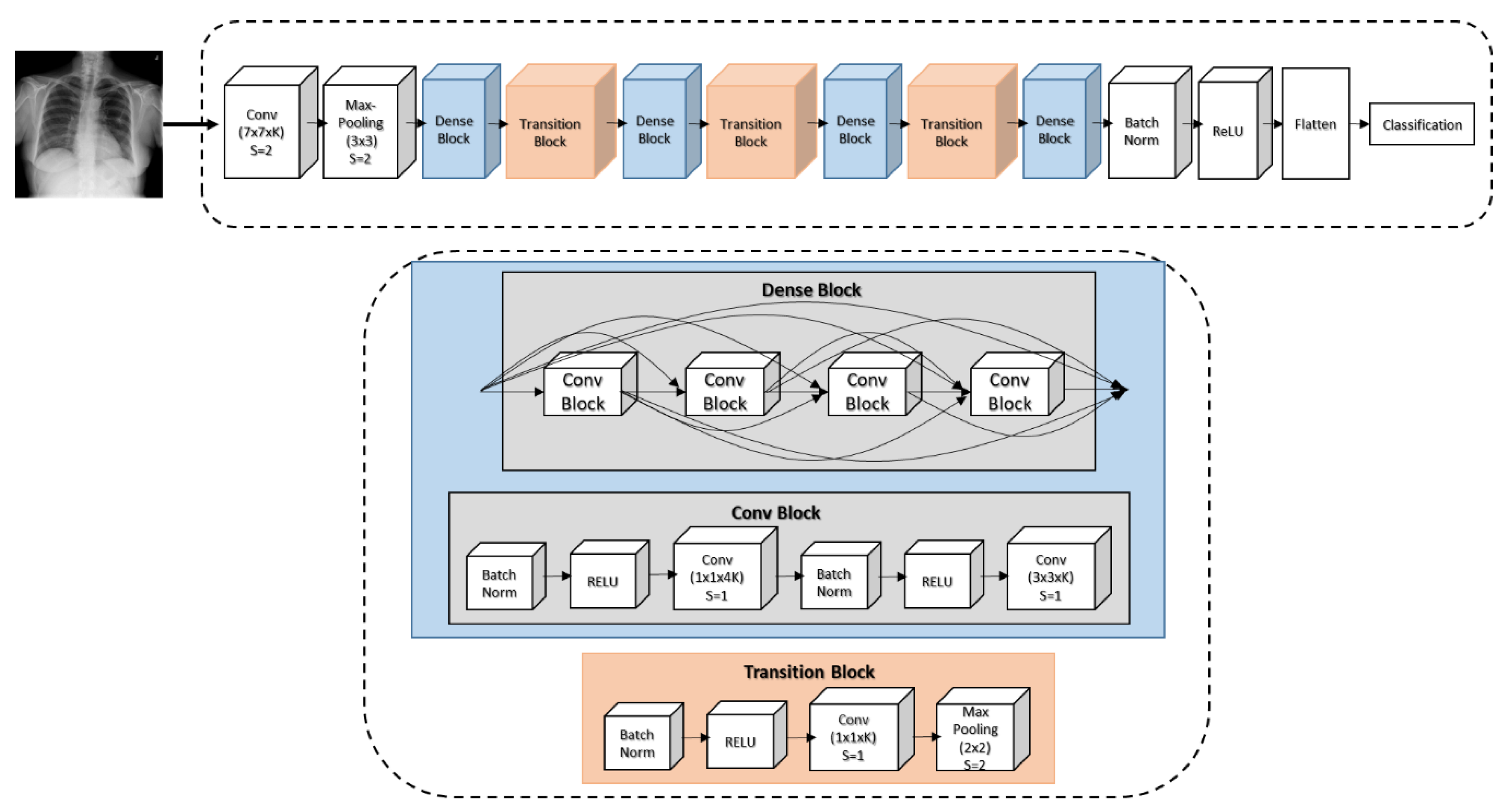
To generate the CAM [50] of the 14 pathological regions and extract deep features, we use the pretrained DenseNet-121 [44], which was trained for pneumonia detection from our targeted ChestX-ray14 dataset. The model architecture of the DenseNet-121 is shown in Figure 2. Compared to the other pretrained CNNs, DenseNet-121 can improve the intake of information and gradients through the network, in which a layer obtains a collective knowledge from all previous layers; passes on its own feature maps to subsequent layers; and then concatenates them into the depth dimension. Thus, the network can be thinner and compact due to having fewer layers. The training error is able to be easily propagated to the previous layers more directly and more computational efficiency tends to be drawn. The network can also learn more diversified and richer feature patterns as the classifier in DenseNet uses features from all complexity levels giving more smooth decision boundaries when training data is insufficient.
The X-ray input image is encoded by a densely connected CNN, similar to DenseNet’s in [43]. At the first stage, we resize the X-ray image into a 224 × 224 grid to be fed into the pretrained DenseNet-121. The weights of DenseNet-121 are initialized with a pretrained model on ImageNet [7] using Adam standard parameters [51]. Next, we freeze all the weights from lower convolutional layers, replace the final fully connected layer with the fully connected layers of a 14-dimensional output, and treat the DenseNet-121 as a fixed feature extractor. In the second stage, we fine-tune the weights from all layers by continuing the back-propagation. Each training iteration aims to optimize the cross-entropy losses through the following equation,
L ( Y , Y ( P ) ) = c = 1 14 Y c log ( Y c ( P ) ) + ( 1 Y c ) log ( 1 Y c ( P ) ) ,
where Y is the ground truth vector and Y ( P ) is the predicted label vector in which each element is binary; 1 and 0 represent the existence and nonexistence of the corresponding diseases, respectively. In this study, the batch size is 16; the momentum is 0.9 (as an optimizer); the initial learning rate is 0.001, which decays by a factor of 10 after each iteration during the validation loss process; and the maximum number of iterations is 50,000.

3.2. Feature Integration

After extracting all the features, we obtain the feature set F = { F S I F T , F G I S T , F L B P , F H O G , F c o n v 1 , F c o n v 2 ,   F c o n v 3 , F c o n v 4 , F c o n v 5 } . To use the best feature integration efficiently, we first evaluate the performances of each descriptor. Features with a high classification performance are selected for the following combinations. Those features are kept if the classification accuracy improves and they are discarded otherwise. Finally, we obtain the best combination of features, denoted as F s . All extracted features are first normalized between 0 and 1 by F L 2 = F | | F | | 2 , where | | F | | = | F 1 | 2 + | F 2 | 2 + + | F n | 2 , and are then concatenated to the final feature representation: F s = { F i L 2 ,   i = 1 , 2 , , N } , where N is the number of selected features.

3.3. Supervised Learning Classifiers

At the final stage, we select a collection of classifiers in a supervised manner to quantitatively evaluate the representative capability of the integrated features, as follows.
  • Gaussian discriminant analysis (GDA) [52]: based on the generative learning algorithm property, we learn the model P ( y ) distributed according to Bernoulli and P ( x | y = k ) , where k is one of the 14 classes distributed according to the multivariate normal distribution; then, P ( y | x ) can be expressed as Sigmoid function.
  • K-nearest neighbor (KNN) [53]: we initialize K = 30 for the number of neighbors to capture and locate similar data points. We gradually increase the value of K so that our KNN predictions become more stable and accurate based on majority voting and averaging.
  • Naïve Bayes [54]: based on the so-called Bayesian theorem, which calculates the posterior probability P ( c | x ) from ( x ) , P ( c ) , and P ( x | c ) , the Naïve Bayes assumes that the effect on a given class ( x ) (x is independent of the predictor, called class conditional independence.
  • Support vector machine (SVM) [55]: we apply SVM algorithms to find an optimal hyperplane acting as a decision boundary in N-dimensional space that can distinctly classify our feature points. We maximize the margin of the classifier when support vectors affect the position and orientation of the hyperplane. The tuning parameters, including the kernel, regularization, and gamma, are carefully chosen.
  • Adaptive boosting (AdaBoost) [56]: we sequentially add a set of weak classifiers and trains using the weighted training data. First, we initialize the weight for each data point, fit weak classifiers to the dataset, and compute the weight of all weak classifiers. After 100 iterations, we obtain the final prediction with the updated weight for each classifier by the formula F ( x ) = s i g n ( n = 1 N W n f n ( x ) ) , where f n is the n t h weak classifier and W n is the corresponding weight.
  • Random Forest [57]: this comprises multiple random decision trees. A random sample from our original dataset forms into each tree. A subset of K features presenting each tree node d is randomly selected to generate the best split. Then, we split the node into daughter nodes and repeating these steps n times to create n trees.
  • Extreme learning machine (ELM) [58]: the ELM includes an input layer, a hidden layer, and an output layer. We set the specific number of hidden neurons, randomize the weight and the bias between input and hidden layers in the execution process, calculate the weight between hidden and output layers by the Moore–Penrose pseudoinverse with a sigmoid activation function, and fit the results with the least-squares method.

4. Experimental Results

4.1. ChestX-Ray14 Dataset and Preprocessing

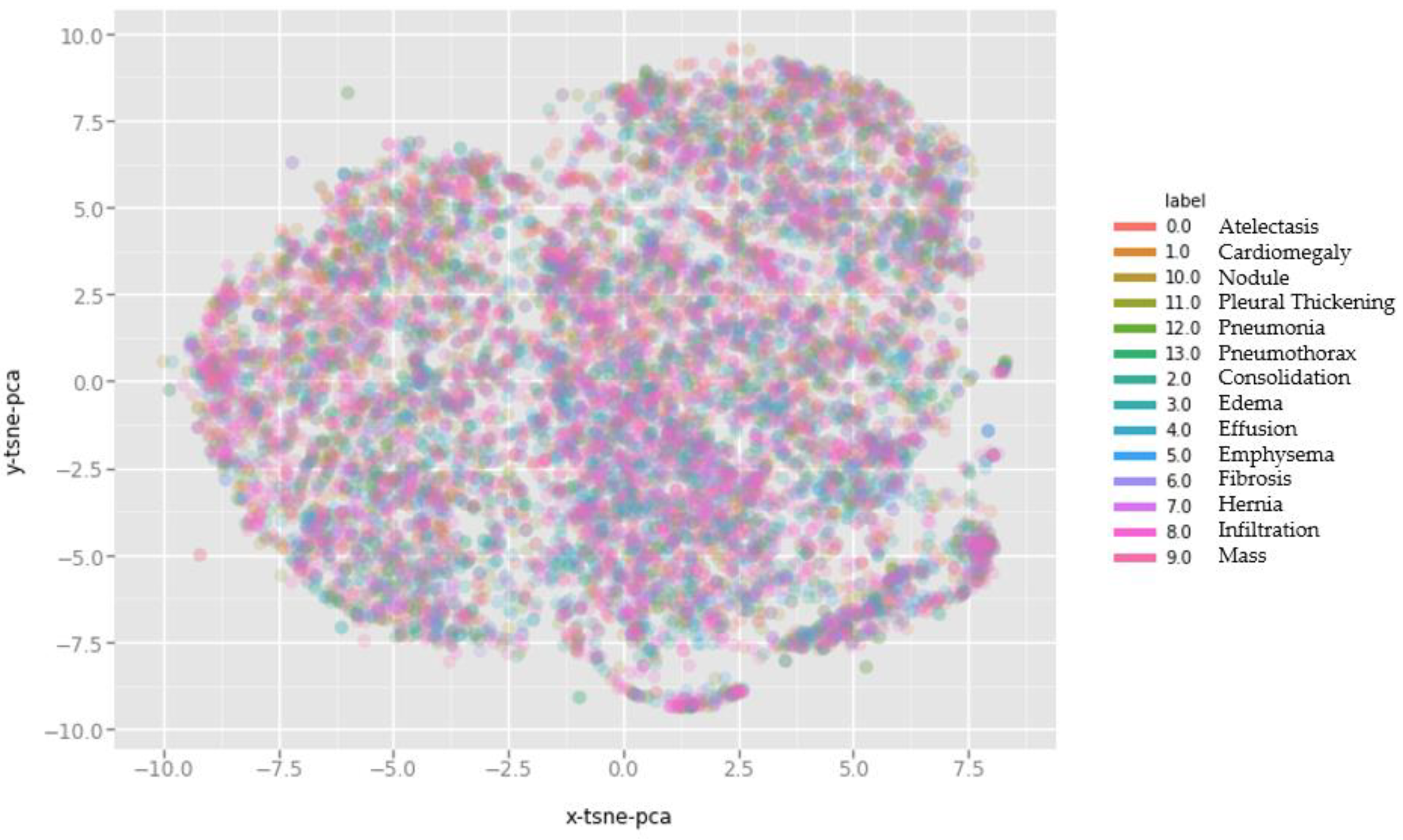
To verify the efficacy of our proposed approach, we conduct experiments on the publicly available ChestX-ray14 dataset recently introduced in [4]. With a total of 112,120 X-ray images acquired from 30,805 unique patients with 14 disease labels, it is the largest collection of front-view chest radiographs to date. Each image is marked by a single or multiple labels based on the radiology reports, with 90% accuracy. Furthermore, 984 labeled bounding boxes (B-Box) are provided by board-certified radiologists. Thus, we select these 984 images as “annotated” for testing CAM visualization and the remaining 111,240 “unannotated” images for training the DenseNet-121 model. We show the complex and diverse distribution of 10,000 sampled images by plotting t-distributed stochastic neighboring entities (t-SNE) [59] and conducting a principle component analysis (PCA) [60] (Figure 3).
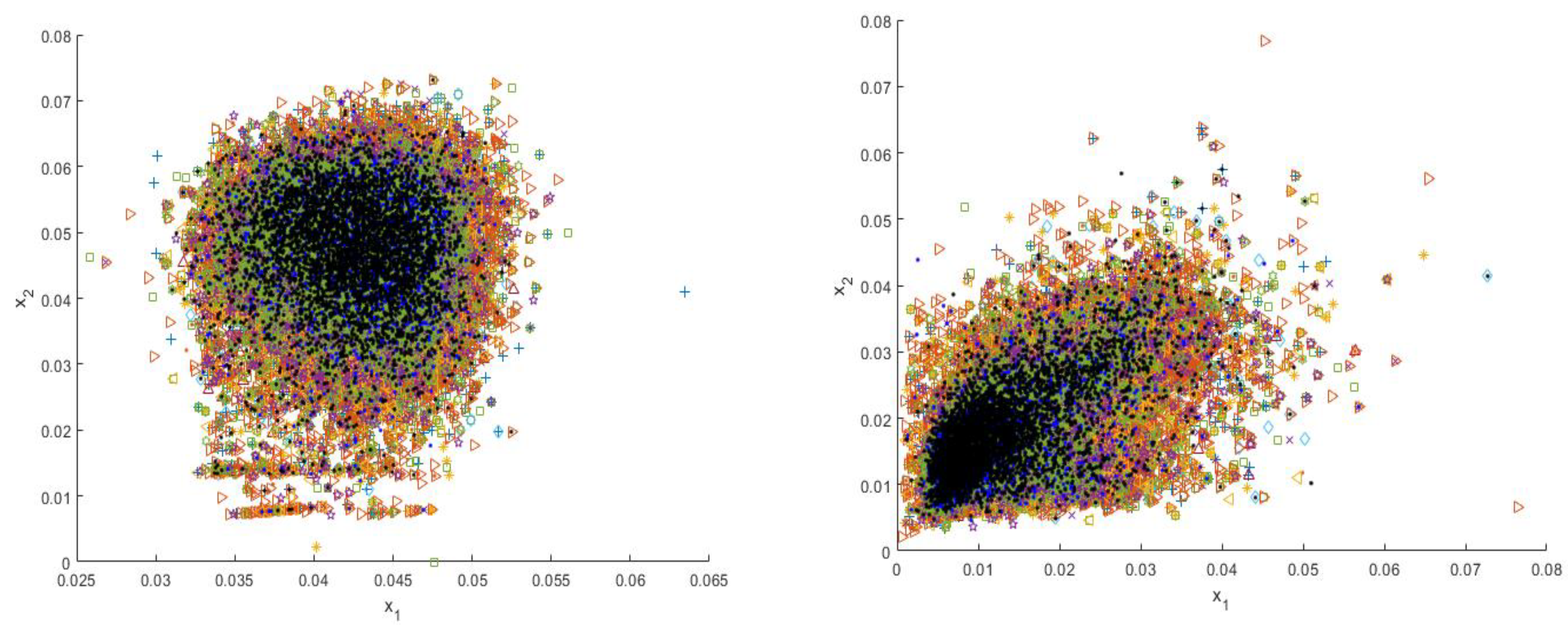
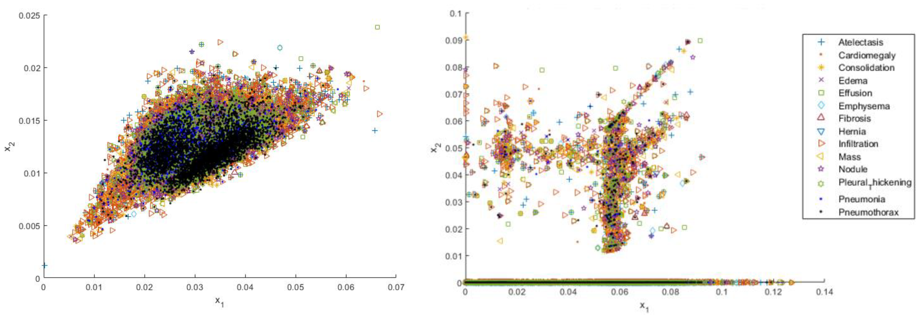
Before inputting images into the DensNet-121 model (Figure 2), we downscale the original 1024 × 1024 PNG images to 224 × 224 PNG, and we normalize them into the range [−1,1] based on the mean and standard deviations of the images. We also augment the training and validation data with batch augmentation and random horizontal flipping methods. In contrast, to extract features from different perspectives based on our proposed shallow descriptors (Figure 4), we keep the original size of the images and do not apply any data augmentation techniques.
We used Python 3.6 for (i) both handcrafted and deep feature extractions and (ii) implementation of the deep pretrained DenseNet-121 model for CAM visualization and classification tasks of 14 thoracic diseases with TensorFlow 1.8.0 deep learning framework of CUDA 9 and cuDNN 7.5 dependencies. In the latter part, we adopted the different classifiers implemented in Matlab 2018b. 10-fold cross-validation was also applied for the classifiers. The total computation time costs for our proposed massive experiments took 143.9 h on a system with an i7-4770K 4-core CPU, 32G of memory, and a GPU, GeForce GTX 1070.

4.2. CAM Visualization

After extracting the activation weights from the final convolutional layer, we can generate the disease heat-maps for each pathology. We obtain the feature map M c of the most salient features by summing up associated weights as follows,
M c = k W c , k F k ,
where F k is the k t h feature map and W c , k is the weight of the final convolutional layer at the feature map k leading to pathology c . We are able to localize pathologies using CAM by highlighting the pathological regions of the X-ray images that are important for performing a specific disease classification. Despite the small number of annotated bounding boxes (984 instances) compared to the entire dataset, it is sufficient to achieve a rational estimate on the disease localization performance of our proposed framework. Figure 5 shows several CAM visualization examples.

4.3. Classification Results

Table 1 and Table 2 show the obtained classification accuracies and F1-scores, respectively. As previously mentioned, four types of shallow local features (SIFT, GIST, LBP, and HOG) are designed to describe image patches from different perspectives. We divide the dataset as 80% for training and 20% for testing. As the first integration strategy, we can see that the classification accuracy of the shallow feature integration is higher than that of each single feature. Furthermore, from the experiments we observe that the classification accuracies keep increasing from Conv1 to Conv5, because the features of shallow layers of deep CNN models are typically basic and shared, preventing the differentiation of the information in X-ray images. Therefore, we disregard the integration of Conv1 to Conv4 with our proposed handcrafted features. The results of Conv5 features, which are integrated with either each single feature descriptor or all the conventional features, are superior to those obtained in the first integration strategy. Regarding the performance of the supervised classifiers at the last stage of our approach, ELM works best among all the single and integrated features, followed by AdaBoost. Figure 6 summarizes the classification results achieved by the seven supervised classifiers.
To accurately compare our proposed approach with the reference baseline model in the classification of all 14 pathologies, we divided the dataset as follows; 70% for training, 10% for validation, and 20% for testing used for the pretrained DenseNet-121; the preprocessing step is described in Section 4.1. The feature integration approach reaches 84.62% classification accuracy, which is higher than the 80.97% accuracy of the pretrained DenseNet-121 model. The experiment reveals the effectiveness of the feature integration strategy in extracting representative and discriminative features to describe X-ray images. Table 3 indicates that our pretrained DenseNet-121 model achieved very competitive accuracies in the diagnosis of the 14 thorax diseases. Note that the authors of [61] trained their model with 180,000 images from the PLCO dataset [62] as extra training data.

5. Conclusions and Future Work

The early diagnosis and treatment of lung disease are essential to prevent deaths worldwide. In this study, we propose a novel framework to integrate multiple features from both shallow and deep features. Representative and discriminative features are obtained to distinguish 14 pathologies from the public ChestX-ray14 dataset after conducting comprehensive experiments. We were able to generate the disease heat-maps despite having a limited number of annotated bounding boxes of pathologies. In addition, our approach yielded competitive classification accuracies compared with the baseline approach. In the future, we will focus on exploiting different shallow feature descriptors and deep features, learning the feature representation, and incorporating them in an end-to-end manner to improve the classification performance.

Author Contributions

The work described in this article is the collaborative development of all authors. J.G. contributed to the idea of data processing and designed the algorithm. T.K.K.H. made contributions to data processing and analysis. J.G. and T.K.K.H participated in the writing of the paper.

Funding

This work was supported by the Brain Research Program through the National Research Foundation of Korea (NRF), funded by the Ministry of Science, ICT & Future Planning (NRF-2019M3C7A1020406), the Engineering Research Center (ERC) Program of Extreme Exploitation of Dark Data through the Korean Government (MSIT) (NRF-2018R1A5A1060031) and the Basic Science Research Program through the NRF, funded by the Ministry of Education (NRF-2017R1D1A1B03036423).

Acknowledgments

The authors would like to note that some part of work was done when J.G. was in Seoul National University Hospital, and we express our gratitude for the valuable and constructive comments made by Lee, M., Kim, H., Hwang, E.-J., and Park, C.-M.

Conflicts of Interest

The authors declare no conflict of interest.

References

  1. Brenner, D.R.; McLaughlin, J.R.; Hung, R.J. Previous lung diseases and lung cancer risk: A systematic review and meta-analysis. PLoS ONE 2011, 6, e17479. [Google Scholar] [CrossRef] [PubMed]
  2. Ruuskanen, O.; Lahti, E.; Jennings, L.C.; Murdoch, D.R. Viral pneumonia. Lancet 2011, 377, 1264–1275. [Google Scholar] [CrossRef]
  3. Litjens, G.; Kooi, T.; Bejnordi, B.E.; Setio, A.A.A.; Ciompi, F.; Ghafoorian, M.; Sánchez, C.I. A survey on deep learning in medical image analysis. Med. Imag. Anal. 2017, 42, 60–88. [Google Scholar] [CrossRef] [PubMed] [Green Version]
  4. Wang, X.; Peng, Y.; Lu, L.; Lu, Z.; Bagheri, M.; Summers, R.M. Chest X-ray8: Hospital-scale chest X-ray database and benchmarks on weakly-supervised classification and localization of common thorax diseases. In Proceedings of the IEEE Conference on Computer Vision and Pattern Recognition, Honolulu, HI, USA, 21–26 July 2017. [Google Scholar]
  5. Liu, C.; Mao, J.; Sha, F.; Yuille, A.L. Attention correctness in neural image captioning. In Proceedings of the AAAI Conference on Artificial Intelligence, San Francisco, CA, USA, 4–9 February 2017. [Google Scholar]
  6. Ba, J.; Mnih, V.; Kavukcuoglu, K. Multiple object recognition with visual attention. arXiv 2014, arXiv:1412.7755. [Google Scholar]
  7. Krizhevsky, A.; Sutskever, I.; Hinton, G.E. Imagenet classification with deep convolutional neural networks. In Proceedings of the Advances in Neural Information Processing Systems, Lake Tahoe, NV, USA, 3–6 December 2012. [Google Scholar]
  8. Simonyan, K.; Zisserman, A. Very deep convolutional networks for large-scale image recognition. In Proceedings of the International Conference on Learning Representations, Banff, AB, Canada, 14–16 April 2015. [Google Scholar]
  9. Zhou, B.; Lapedriza, A.; Xiao, J.; Torralba, A.; Oliva, A. Learning deep features for scene recognition using places database. In Proceedings of the Advances in Neural Information Processing Systems, Montreal, QC, Canada, 6–13 December 2014. [Google Scholar]
  10. Schroff, F.; Kalenichenko, D.; Philbin, J. Facenet: A unified embedding for face recognition and clustering. In Proceedings of the IEEE Conference on Computer Vision and Pattern Recognition, Boston, MA, USA, 7–12 June 2015. [Google Scholar]
  11. Girshick, R.; Donahue, J.; Darrell, T.; Malik, J. Region-based convolutional networks for accurate object detection and segmentation. IEEE Trans. Pattern Anal. Mach. Intell. 2015, 38, 142–158. [Google Scholar] [CrossRef]
  12. Russakovsky, O.; Deng, J.; Su, H.; Krause, J.; Satheesh, S.; Ma, S.; Huang, Z.; Karpathy, A.; Khosla, A.; Bernstein, M.; et al. Imagenet large scale visual recognition challenge. Int. J. Comput. Vis. 2015, 115, 211–252. [Google Scholar] [CrossRef]
  13. Lin, T.-Y.; Maire, M.; Belongie, S.; Hays, J.; Perona, P.; Ramanan, D.; Dollr, P.; Zitnick, L. Microsoft coco: Common objects in context. In Proceedings of the European Conference on Computer Vision, Zurich, Switzerland, 6–12 September 2014. [Google Scholar]
  14. Johnson, J.; Karpathy, A.; Fei-Fei, L. DenseCap: Fully convolutional localization networks for dense captioning. In Proceedings of the IEEE Conference on Computer Vision and Pattern Recognition, Las Vegas, NV, USA, 26 June–1 July 2016. [Google Scholar]
  15. Krishna, R.; Zhu, Y.; Groth, O.; Johnson, J.; Hata, K.; Kravitz, J.; Chen, S.; Kalantidis, Y.; Li, L.-J.; Shamma, D.A.; et al. Visual Genome: Connecting language and vision using crowdsourced dense image annotations. Int. J. Comput. Vis. 2017, 123, 32–73. [Google Scholar] [CrossRef]
  16. Roth, H.R.; Lu, L.; Seff, A.; Cherry, K.M.; Hoffman, J.; Wang, S.; Liu, J.; Turkbey, E.; Summers, R.M. A new 2.5D representation for lymph node detection using random sets of deep convolutional neural network observations. In Proceedings of the International Conference on Medical Image Computing and Computer Assisted Intervention, Boston, MA, USA, 14–18 September 2014. [Google Scholar]
  17. Shin, H.; Roth, H.; Gao, M.; Lu, L.; Xu, Z.; Nogues, I.; Yao, J.; Mollura, D.; Summers, R. Deep convolutional neural networks for computer-aided detection: CNN architectures, dataset characteristics and transfer learnings. IEEE Trans. Med. Imag. 2016, 35, 1285–1298. [Google Scholar] [CrossRef]
  18. Setio, A.; Ciompi, F.; Litjens, G.; Gerke, P.; Jacobs, C.; van Riel, S.; Wille, M.; Naqibullah, M.; Snchez, C.; van Ginneken, B. Pulmonary nodule detection in ct images: False positive reduction using multi-view convolutional networks. IEEE Trans. Med. Imag. 2016, 35, 1160–1169. [Google Scholar] [CrossRef]
  19. Dou, Q.; Chen, H.; Yu, L.; Zhao, L.; Qin, J.; Wang, D.; Mok, V.; Shi, L.; Heng, P. Automatic detection of cerebral microbleeds from mr images via 3d convolutional neural networks. IEEE Trans. Med. Imag. 2016, 35, 1182–1195. [Google Scholar] [CrossRef]
  20. Jamaludin, A.; Kadir, T.; Zisserman, A. SpineNet: Automatically pinpointing classification evidence in spinal MRIs. In Proceedings of the International Conference on Medical Image Computing and Computer Assisted Intervention, Athens, Greece, 17–21 October 2016. [Google Scholar]
  21. Esteva, A.; Kuprel, B.; Novoa, R.A.; Ko, J.; Swetter, S.M.; Blau, H.M.; Thrun, S. Dermatologist-level classification of skin cancer with deep neural networks. Nature 2017, 542, 115–118. [Google Scholar] [CrossRef] [PubMed]
  22. Roth, H.; Lu, L.; Farag, A.; Shin, H.-C.; Liu, J.; Turkbey, E.B.; Summers, R.M. DeepOrgan: Multi-level deep convolutional networks for automated pancreas segmentation. In Proceedings of the International Conference on Medical Image Computing and Computer Assisted Intervention, Munich, Germany, 5–9 October 2015. [Google Scholar]
  23. Lowe, D.G. Distinctive image features from scale-invariant keypoints. Int. J. Comput. Vis. 2004, 60, 91–110. [Google Scholar] [CrossRef]
  24. Ojala, T.; Pietikäinen, M.; Mäenpää, T. Multiresolution gray-scale and rotation invariant texture classification with local binary patterns. IEEE Trans. Pattern Anal. Mach. Intell. 2002, 7, 971–987. [Google Scholar] [CrossRef]
  25. Dalal, N.; Triggs, B. Histograms of oriented gradients for human detection. In Proceedings of the IEEE Conference on Computer Vision and Pattern Recognition, San Diego, CA, USA, 20–26 June 2005. [Google Scholar]
  26. Negrel, R.; Picard, D.; Gosselin, P.H. Evaluation of second-order visual features for land-use classification. In Proceedings of the 12th IEEE International Workshop on Content-Based Multimedia Indexing, Klagenfurt, Austria, 8–20 June 2014. [Google Scholar]
  27. Zhong, Y.; Zhu, O.; Zhang, L. Scene classification based on the multifeature fusion probabilistic topic model for high spatial resolution remote sensing imagery. IEEE Trans. Geosci. Remote Sens. 2015, 53, 6207–6222. [Google Scholar] [CrossRef]
  28. Penatti, O.A.; Nogueira, K.; Santos, J.A.D. Do deep features generalize from everyday objects to remote sensing and aerial scenes domains? In Proceedings of the IEEE Conference on Computer Vision and Pattern Recognition Workshops, Boston, MA, USA, 8–10 June 2015. [Google Scholar]
  29. Vu, T.H.; Mousavi, H.S.; Monga, V.; Rao, G.; Rao, U.A. Histopathological image classification using discriminative feature-oriented dictionary learning. IEEE Trans. Med. Imag. 2015, 35, 738–751. [Google Scholar] [CrossRef] [PubMed]
  30. Otálora, S.; Cruz-Roa, A.; Arevalo, J.; Atzori, M.; Madabhushi, A.; Judkins, A.R.; Depeursinge, A. Combining unsupervised feature learning and riesz wavelets for histopathology image representation: Application to identifying anaplastic medulloblastoma. In Proceedings of the International Conference on Medical Image Computing and Computer-Assisted Intervention, Munich, Germany, 5–9 October 2015. [Google Scholar]
  31. Hu, F.; Xia, G.S.; Hu, J.; Zhang, L. Transferring deep convolutional neural networks for the scene classification of high-resolution remote sensing imagery. Remote Sens. 2015, 7, 14680–14707. [Google Scholar] [CrossRef]
  32. Yosinski, J.; Clune, J.; Bengio, Y.; Lipson, H. How transferable are features in deep neural networks? In Proceedings of the Advances in Neural Information Processing Systems, Montreal, QC, Canada, 8–13 December 2014. [Google Scholar]
  33. Van Ginneken, B.; Setio, A.A.; Jacobs, C.; Ciompi, F. Off-the-shelf convolutional neural network features for pulmonary nodule detection in computed tomography scans. In Proceedings of the 2015 IEEE 12th International Symposium on Biomedical Imaging (ISBI), New York, NY, USA, 16–19 April 2015. [Google Scholar]
  34. Nanni, L.; Ghidoni, S.; Brahnam, S. Ensemble of convolutional neural networks for bioimage classification. Appl. Comput. Inf. 2018. [Google Scholar] [CrossRef]
  35. Mahmood, A.; Bennamoun, M.; An, S.; Sohel, F.; Boussaid, F.; Hovey, R.; Fisher, R.B. Coral classification with hybrid feature representations. In Proceedings of the 2016 IEEE International Conference on Image Processing (ICIP), Phoenix, AZ, USA, 25–28 September 2016. [Google Scholar]
  36. Tang, Y.; Tang, Y.; Sandfort, V.; Xiao, J.; Summers, R.M. TUNA-Net: Task-oriented UNsupervised Adversarial Network for Disease Recognition in Cross-Domain Chest X-rays. arXiv 2019, arXiv:1908.07926. [Google Scholar]
  37. Li, Z.; Wang, C.; Han, M.; Xue, Y.; Wei, W.; Li, L.J.; Fei-Fei, L. Thoracic disease identification and localization with limited supervision. In Proceedings of the IEEE Conference on Computer Vision and Pattern Recognition, Salt Lake City, UT, USA, 18–22 June 2018. [Google Scholar]
  38. Salehinejad, H.; Valaee, S.; Dowdell, T.; Colak, E.; Barfett, J. Generalization of deep neural networks for chest pathology classification in x-rays using generative adversarial networks. In Proceedings of the 2018 IEEE International Conference on Acoustics, Speech and Signal Processing, Calgary, AB, Canada, 15–20 April 2018. [Google Scholar]
  39. Szegedy, C.; Liu, W.; Jia, Y.; Sermanet, P.; Reed, S.; Anguelov, D.; Erhan, D.; Vanhoucke, V.; Rabinovich, A. Going deeper with convolutions. In Proceedings of the IEEE Conference on Computer Vision and Pattern Recognition, Boston, MA, USA, 7–12 June 2015. [Google Scholar]
  40. He, K.; Zhang, X.; Ren, S.; Sun, J. Deep residual learning for image recognition. arXiv 2015, arXiv:1512.03385. [Google Scholar]
  41. Yao, L.; Poblenz, E.; Dagunts, D.; Covington, B.; Bernard, D.; Lyman, K. Learning to diagnose from scratch by exploiting dependencies among labels. arXiv 2017, arXiv:1710.10501. [Google Scholar]
  42. Kumar, P.; Grewal, M.; Srivastava, M.M. Boosted cascaded convnets for multilabel classification of thoracic diseases in chest radiographs. In Proceedings of the International Conference Image Analysis and Recognition, Póvoa de Varzim, Portugal, 27–29 June 2018. [Google Scholar]
  43. Rajpurkar, P.; Irvin, J.; Zhu, K.; Yang, B.; Mehta, H.; Duan, T.; Lungren, M.P. Radiologist-level pneumonia detection on chest X-rays with deep learning. arXiv 2017, arXiv:1711.05225. [Google Scholar]
  44. Wang, H.; Xia, Y. Chestnet: A deep neural network for classification of thoracic diseases on chest radiography. arXiv 2018, arXiv:1807.03058. [Google Scholar]
  45. Wang, X.; Peng, Y.; Lu, L.; Lu, Z.; Summers, R.M. Tienet: Text-image embedding network for common thorax disease classification and reporting in chest X-rays. In Proceedings of the IEEE Conference on Computer Vision and Pattern Recognition, Salt Lake City, UT, USA, 18–22 June 2018. [Google Scholar]
  46. Baltruschat, I.M.; Nickisch, H.; Grass, M.; Knopp, T.; Saalbach, A. Comparison of deep learning approaches for multi-label chest X-ray classification. arXiv 2018, arXiv:1803.02315. [Google Scholar] [CrossRef] [PubMed]
  47. Luo, B.; Jiang, S.; Zhang, L. Indexing of remote sensing images with different resolutions by multiple features. IEEE J. Select. Topics Appl. Earth Observ. Remote Sens. 2013, 6, 1899–1912. [Google Scholar] [CrossRef]
  48. Li, E.; Xia, J.; Lin, P.D.C.; Samat, A. Integrating multilayer features of convolutional neural networks for remote sensing scene classification. IEEE Trans. Geosci. Remote Sens. 2017, 55, 5653–5665. [Google Scholar] [CrossRef]
  49. Oliva, A.; Torralba, A. Modeling the shape of the scene: A holistic representation of the spatial envelope. Int. J. Comput. Vis. 2004, 42, 145–175. [Google Scholar] [CrossRef]
  50. Zhou, B.; Khosla, A.; Lapedriza, A.; Oliva, A.; Torralba, A. Learning deep features for discriminative localization. In Proceedings of the IEEE Conference on Computer Vision and Pattern Recognition, Las Vegas, NV, USA, 26 June–1 July 2016. [Google Scholar]
  51. Kingma, D.P.; Ba, J. Adam: A method for stochastic optimization. arXiv 2014, arXiv:1412.6980. [Google Scholar]
  52. Ju, J.; Kolaczyk, E.D.; Gopal, S. Gaussian mixture discriminant analysis and sub-pixel land cover characterization in remote sensing. Remote Sens. Environ. 2003, 84, 550–560. [Google Scholar] [CrossRef]
  53. Weinberger, K.Q.; Saul, L.K. Distance metric learning for large margin nearest neighbor classification. In Proceedings of the Advances in Neural Information Processing Systems, Vancouver, BC, Canada, 4–7 December 2006. [Google Scholar]
  54. Murphy, K.P. Naive Bayes Classifiers; University of British Columbia: Vancouver, BC, Canada, 2006. [Google Scholar]
  55. Fung, G.M.; Mangasarian, O.L. Multicategory proximal support vector machine classifiers. Mach. Learn. 2005, 59, 77–97. [Google Scholar] [CrossRef]
  56. Sun, Y.; Liu, Z.; Todorovic, S.; Li, J. Adaptive boosting for SAR automatic target recognition. IEEE Trans. Aerosp. Electron. Syst. 2007, 43, 112–125. [Google Scholar] [CrossRef]
  57. Pal, M. Random forest classifier for remote sensing classification. Int. J. Remote Sens. 2005, 26, 217–222. [Google Scholar] [CrossRef]
  58. Huang, G.B.; Zhou, H.; Ding, X.; Zhang, R. Extreme learning machine for regression and multiclass classification. IEEE Trans. Syst. Man Cybern. 2011, 42, 513–529. [Google Scholar] [CrossRef] [PubMed]
  59. Abdelmoula, W.M.; Balluff, B.; Englert, S.; Dijkstra, J.; Reinders, M.J.; Walch, A.; Lelieveldt, B.P. Data-driven identification of prognostic tumor subpopulations using spatially mapped t-SNE of mass spectrometry imaging data. Proc. Natl. Acad. Sci. USA 2016, 113, 12244–12249. [Google Scholar] [CrossRef] [PubMed] [Green Version]
  60. Abdi, H.; Williams, L.J. Principal component analysis. Wiley Interdiscip. Rev. Comput. Stat. 2010, 2, 433–459. [Google Scholar] [CrossRef]
  61. Guendel, S.; Grbic, S.; Georgescu, B.; Liu, S.; Maier, A.; Comaniciu, D. Learning to recognize abnormalities in chest X-rays with location-aware dense networks. In Proceedings of the Iberoamerican Congress on Pattern Recognition, Madrid, Spain, 19–22 November 2018. [Google Scholar]
  62. Team, P.P.; Gohagan, J.K.; Prorok, P.C.; Hayes, R.B.; Kramer, B.S. The Prostate, Lung, Colorectal and Ovarian (PLCO) cancer screening trial of the National Cancer Institute: History, organization, and status. Controll. Clinic. Trials 2000, 21, 251S–272S. [Google Scholar]
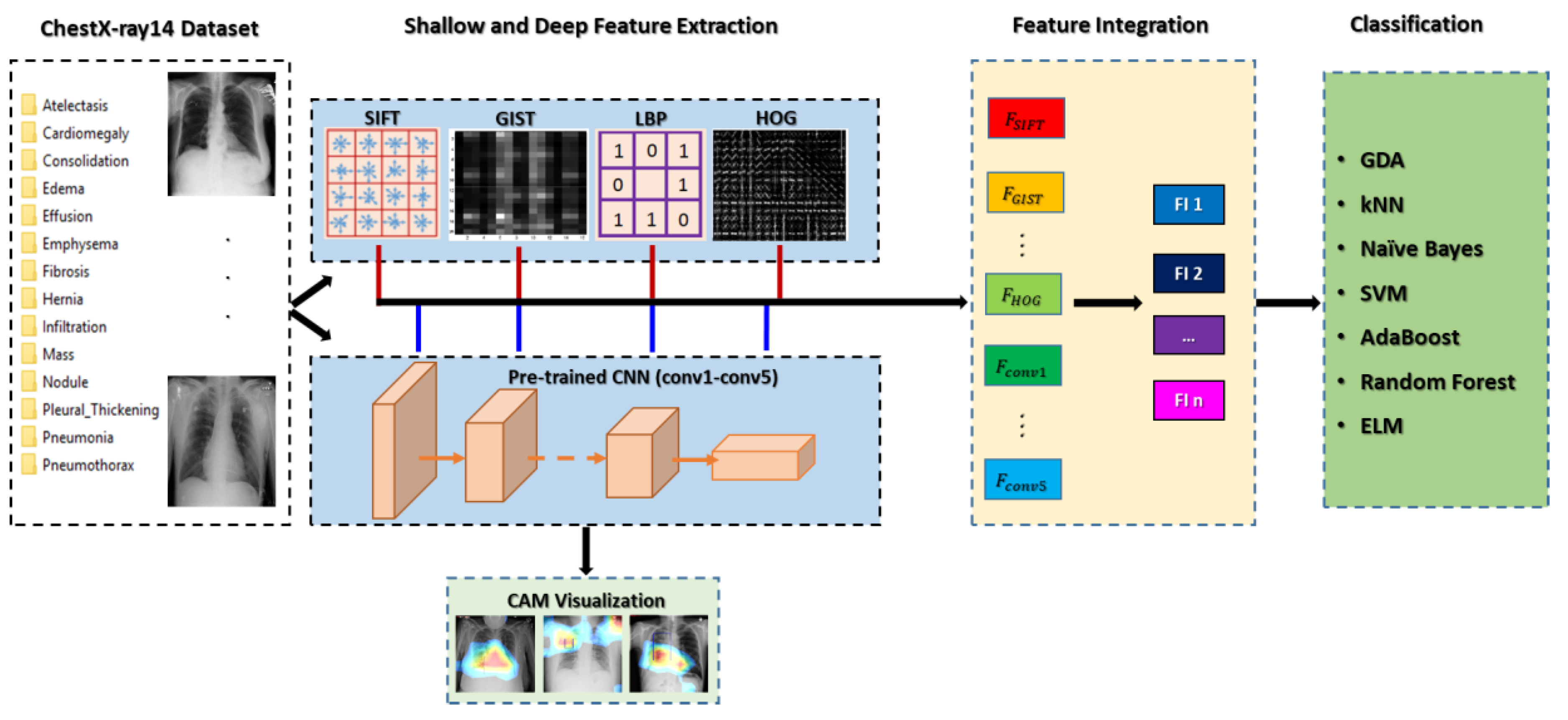
Figure 1. Framework of the proposed multiple feature integration approach.
Applsci 09 04130 g001
Figure 2. DenseNet-121 architecture for generating class activation map (CAM) results and classifying the 14 pathologies.
Applsci 09 04130 g002
Figure 3. t-distributed stochastic neighboring entities (t-SNE) dimensions colored by digits with the usage of PCA.
Applsci 09 04130 g003
Figure 4. Distributions of four types of shallow features including SIFT, GIST, local binary pattern (LBP), and HOG (from left to right, top to bottom, respectively).
Applsci 09 04130 g004aApplsci 09 04130 g004b
Figure 5. Example CAM results based on Pretrained DenseNet-121, which extracts the weight activations from the last convolutional layers and generate CAMs for 14 pathologies.
Applsci 09 04130 g005
Figure 6. Classification results using the integration of all features (i.e., FI 3) among the classifiers.
Applsci 09 04130 g006
Table 1. Accuracies of the classifiers using the feature(s) w/ or w/o the feature integration approach.
FeatureDataset Division
( ): No. of Images
Accuracy
GDAKNNNaïve BayesSVMAda-BoostRandom ForestELM
SIFTTraining:
80% (89,696)
Testing:
20% (22,424)
0.57200.60260.65620.55980.64510.66210.7669
GIST0.58500.60300.65570.57320.64010.67100.7227
LBP059410.60090.64400.58650.64710.72100.7828
HOG0.59470.60120.64870.58970.64890.67510.7837
FI 1SIFT+GIST+LBP+HOG0.60390.62050.65870.61120.65510.69020.7941
FI 2Conv5+SIFT0.57530.55690.48030.60650.64010.64520.6742
Conv5+GIST0.60060.55990.48080.61280.64510.63090.7115
Conv5+LBP0.60580.56070.48170.62130.65190.66490.8115
Conv5+HOG0.59010.55770.48070.59920.65510.65010.8105
FI 3Conv5+SIFT+GIST+LBP+HOG0.68340.63320.60520.74780.79520.77010.8462
Fully pretrained DenseNet121Training:
70% (78,484)
Validation:
10% (11,212)
Testing:
20% (22,424)
0.8097
Table 2. Classification F1-scores using feature integration approach among seven classifiers.
FeatureDataset Division
( ): No. of images
F1-score
GDAKNNNaïve BayesSVMAda-BoostRandom
Forest
ELM
SIFTTraining:
80% (89,696)
Testing:
20% (22,424)
0.72760.76460.79240.71240.79370.82110.8686
GIST0.74360.76510.79210.72920.79370.81010.8227
LBP0.75520.76270.78350.74540.79370.81670.8328
HOG0.75520.76270.78690.74450.79370.81000.8262
FI 1SIFT+GIST+LBP+HOG0.76620.57660.79420.77470.79370.80110.8520
FI 2Conv5+SIFT0.70880.60560.76930.79370.79010.81100.6742
Conv5+GIST0.71260.60620.77660.79570.77150.84440.7115
Conv5+LBP0.70090.60760.78630.79370.81060.86460.8115
Conv5+HOG0.70980.60600.76060.79370.81020.84450.8105
FI 3Conv5+SIFT+GIST+LBP+HOG0.84130.75410.71380.86610.90380.88580.9413
Fully pretrained DenseNet121Training:
70% (78,484)
Validation:
10% (11,212)
Testing:
20% (22,424)
0.8838
Table 3. AUC comparison of the 14 pathologies classification in the ChestX-ray14 literature.
PathologyWang et al. [4]Yao et al. [41]Gundel et al. [61]Wang et al. [44]Proposed
Atelectasis0.7160.7720.7670.7430.795
Cardiomegaly0.8070.9040.8830.8750.887
Effusion0.7840.8590.8280.8110.875
Infiltration0.6090.6950.7090.6770.703
Mass0.7060.7920.8210.7830.835
Nodule0.6710.7170.7580.6980.716
Pneumonia0.6330.7130.7310.6960.742
Pneumothorax0.8060.8410.8460.8100.863
Consolidation0.7080.7880.7450.7230.786
Edema0.8350.8820.8350.8330.892
Emphysema0.8150.8290.8950.8220.875
Fibrosis0.7690.7670.8180.8040.756
Pleural Thickening0.7080.7650.7610.7510.774
Hernia0.7670.9140.8960.8990.836
Average0.7380.8010.8070.7810.8097