Article

Fault Diagnosis Method for Engine Control System Based on Probabilistic Neural Network and Support Vector Machine

1
College of Energy and Power Engineering, Nanjing University of Aeronautics and Astronautics, Nanjing 210016, China
2
AECC Sichuan Gas Turbine Establishment, Chengdu 610500, China
*
Author to whom correspondence should be addressed.
Appl. Sci. 2019, 9(19), 4122; https://doi.org/10.3390/app9194122
Submission received: 7 August 2019 / Revised: 20 September 2019 / Accepted: 23 September 2019 / Published: 2 October 2019

Abstract

:
Due to the poor working conditions of an engine, its control system is prone to failure. If these faults cannot be treated in time, it will cause great loss of life and property. In order to improve the safety and reliability of an aero-engine, fault diagnosis, and optimization method of engine control system based on probabilistic neural network (PNN) and support vector machine (SVM) is proposed. Firstly, using the German 3 W piston engine as a control object, the fault diagnosis scheme is designed and introduced briefly. Then, the fault injection is performed to produce faults, and the data sample for engine fault diagnosis is established. Finally, the important parameters of PNN and SVM are optimized by particle swarm optimization (PSO), and the results are analyzed and compared. It shows that the engine fault diagnosis method based on PNN and SVM can effectively diagnose the common faults. Under the optimization of PSO, the accuracy of PNN and SVM results are significantly improved, the classification accuracy of PNN is up to 96.4%, and the accuracy of SVM is up to 98.8%, which improves the application of them in fault diagnosis technology of aero-piston engine control system.

1. Introduction

Due to the complex structure of the aviation piston engine, its control system must be a complex system with multi-loop, multi-variable, and non-linear. Currently, adopting Full-Authority Digital Electronic Control (FADEC) [1] has become an inevitable trend in the development of aero-engine control system technology. Under the poor working conditions of the engine, the sensors, the execution structure and the internal components of the engine control system will inevitably fail during operation. If the faults cannot be diagnosed and eliminated in time, it will cause huge economic losses while endangering personal safety. Therefore, there is an urgent need to improve the reliability and safety of the aviation piston engine control system. At present, the main measure taken to improve system reliability and safety is to improve the reliability of engine components [2]. However, the reliability of components will inevitably decrease as time goes by. Therefore, if the system faults can be detected, separated and corrected by automatic fault detection and diagnosis technology as early as possible, it can effectively improve the safety and stability of the system and avoid unnecessary losses [3,4]. In this aspect, researchers have done a lot of work. For example, Bin Jiang et al. proposed some fault-tolerant tracking-control schemes based on the adaptive-control technique [5,6]. The efficiency of the approaches are verified by experiment. Mohammed Chadli et al. proposed a new design approach for distributed state estimation and fault detection and isolation (FDI) filters, which can detect the fault signal effectively [7].
With the research and development of intelligent algorithms such as neural networks and support vector machines, intelligent diagnostic techniques have emerged since the early 1980s and are gradually applied in various fields. Tthe techniques aroused the attention of engine researchers. In 1999, Matthias Rychetsky et al. applied support vector machine to the actual detection of engine knock [8]. In 2002, researchers in Nanjing University of Aeronautics and Astronautics used probabilistic neural networks to qualitatively diagnose several prototype faults of aero engines. The results showed that though the noise of the measured parameters was large, the probabilistic neural network still had high diagnostic accuracy and could minimize the losses from misdiagnosis [9]. In 2011, Prashant P. Bedekar et al. applied the neural network based on Hebb learning rules to the fault diagnosis of power systems, and the effectiveness of the method has been verified by various testing systems [10]. In 2016, a researcher used the support vector machine to establish the main fuel flow estimation model of the engine, and the effectiveness of the fault diagnosis system designed by them was verified by semi-physical simulation experiments. It promoted the application of artificial intelligence algorithm in engine fault diagnosis [11]. In 2018, Ding lei studied the feature vector which was based on IMF band energy characteristics and used the support vector machine to realize the identification of different degrees of the engine pistons’ failure [12]. The result promotes the application of support vector machine in the fault diagnosis of piston engines. At present, the use of intelligent diagnostic technology to diagnose engine faults has become a major trend. Improving the accuracy of fault diagnosis results and the applicability of diagnostic techniques has become the primary goal of researchers. With the purpose to improve the accuracy of diagnosis results and improve the safety and reliability of aero engines, this paper proposes a fault diagnosis and optimization method for engine control system based on probabilistic neural network and support vector machine. The experiments’ results show that the engine fault diagnosis method based on probabilistic neural network and support vector machine can effectively diagnose the common faults of the control system. Under the optimization of PSO, the accuracy of PNN and SVM fault diagnosis classification results are significantly improved, the classification accuracy of PNN is up to 96.4%, and the accuracy of SVM is up to 98.8%, which improves the application of PNN and SVM in fault diagnosis technology of aero-piston engine control system. It provides a truly effective method for fault diagnosis of aviation piston engine control systems.

2. Fault Diagnosis Algorithm Selection

There are a variety of algorithms that belong to neural networks, such as feedback neural networks, self-organizing competitive neural networks, and probabilistic neural networks. Compared with other neural networks, probabilistic neural networks are neural networks based on statistical principles. They are equivalent to the optimal Bayes classifier in classification function. The essence of them is a parallel algorithm based on Bayesian minimum risk criterion. At the same time, unlike the traditional multi-layer forward network which needs to use the feedback algorithm to calculate the reverse error propagation, this method is the complete forward calculation process [13]. It has the advantages of short training time, less local optimum, and high classification accuracy.
Support vector machine is a new machine learning method proposed by Vapnic on the basis of statistical learning theory in 1995 [14]. It is based on VC dimension theory and structural risk minimization principle. The algorithm of it is a convex quadratic optimization problem, which can guarantee that the found extremum solution is the global optimal solution. It has unique advantages in solving nonlinear and high dimensional pattern recognition and small sample classification problems [15]. In addition, the support vector machine also has the advantages of strong universal type and simple calculation.
Due to the superior performance of probabilistic neural networks and support vector machines in pattern recognition, they have the potential for diagnosing faults. In this paper, they are chosen to be used to diagnose faults in the 3 W engine control systems.

2.1. Introduction of Probabilistic Neural Network

Probabilistic neural networks are based on the Radical Basis Function (RBF) neural network, and they are developed by combining Bayesian decision and density function estimation theory. Unlike the RBF neural network, probabilistic neural networks are specifically applied to classification problems [8,16]. Since all neural networks are progressive theories which ask the number of samples tends to infinity, theoretically, only the number of training samples is large enough to achieve optimal classification performance.
Bayes Rule was proposed by the British mathematician named with Thomas Bayes in 1763 [17]. Bayesian decision theory is the theoretical basis of probabilistic neural networks. The mathematical expression of the Bayesian formula is in Equation (1).
P ( A i | B ) = P ( A i ) P ( B | A i ) j = 1 n p ( A i ) P ( B | A i ) , i = 1 , 2 , , n
In Equation (1), A 1 to A n form a complete event group, and with each A i there exits P ( A i ) > 0 . Every member of this group is the different cause of event B .
Probabilistic neural networks are mainly composed of input layer, hidden layer, summation layer, and decision layer [18]. The input vector x reaches the hidden layer through the input layer. In this paper, the Gaussian function is used to define the relationship between the input and output of the j-th neuron in the i-th class of the hidden layer. The specific formula is in Equation (2).
Φ i j ( x ) = 1 ( 2 π ) 1 2 σ d e ( x x i j ) ( x x i j ) t σ 2
where the value range i is [1,N]. N represents the total number of classes in the training sample, and d is the dimension of the sample space, x i j represents the j-th neuron center of the sample.
Summation layer weighted average the input from the same layer of implicit layers in the corresponding sample. The specific form is shown with Equation (3), where V i represents the category output of the i-th class, and n represents the number of neurons of the i-th class.
V i = j = 1 n ϕ i j n
Set ω as the weighting coefficient, and the input vector x must be multiplied by the weighting coefficient ω. Then put it into the hidden layer, if x and ω have been normalized to unit length, and then use radial basis operation to obtain the Equation (4).
f ( x , ω i ) = exp [ ( ω i x ) T ( ω i x ) 2 σ 2 ]
where σ represents the smoothing factor of the probabilistic neural network, which has a great influence on the final classification result of the network.

2.2. Introduction of Support Vector Machines

The composition of the support vector machine is simple, usually composed of three layers, including the input layer, the kernel function layer, and the output layer. Among them, the input layer is mainly used to receive data samples that need to be trained. The selection of kernel functions in the kernel function layer is important which solves the defect of insufficient computing power [19]. As for the output layer, it is mainly affected by the kernel function layer and the influence of the definition of the sample label.
Set x i and x j as the sample points in the data space, and ϕ represents the mapping from the data space to feature space. The process of transformation is as in Equation (5).
( x i , x j ) K ( x i , x j ) = ϕ ( x i ) ϕ ( x j )
In SVM, the kernel function directly affects the final result of SVM processing data classification and nonlinear regression. Therefore, the kernel function of SVM must be carefully selected when applying. The usually used kernel functions are shown as follows.
  • Linear kernel function: K ( x i , x j ) = x i T x j .
  • Polynomial kernel function: K ( x i , x j ) = ( γ x i T x j + r ) p , r > 0 .
  • Radial basis kernel function: K ( x i , x j ) = exp ( r x i x j 2 ) , r > 0 .
  • Two-layer perceptron kernel function: K ( x i , x j ) = tanh ( γ x i T x j + r ) .
When the samples exist crossover, classification hyperplane for SVM cannot be established and the samples may be incorrectly classified. To classify data using SVM under this situation, it is necessary to introduce the slack variables. With this measure, the classification of the data can be achieved in the case of sample misclassification [20]. The slack variable means a non-negative variable ξ i for each data sample point x i , and it represents the distance from the wrong sample point to its corresponding boundary hyperplane.
In Equation (6), W 2 represents the objective function. Its value will be increased by the introducing of the slack variables in cross samples, which will increase the loss of classification. With the purpose to measure the loss, in this paper, a first-order soft-interval classifier is chosen. By introducing penalty factors into the target optimization function, the optimized function is transformed into the following form.
min { 1 2 W 2 + C i = 1 l ξ i }
Restrictions : { y i ( ( W X ) + b ) ) p ξ i ξ i 0 , ( i = 1 , 2 , , l )
When there is a misclassification, SVM with penalty factors can realize the control of the classification error and classification interval of the data sample. This is the model of C-SVM where C represents the penalty factor, and it indicates the degree of punishment for the misclassified sample. The greater the C value, the greater the penalty and the stricter the misclassification of the sample.
When using C-SVM for classification, it is necessary to select the appropriate parameter C firstly. Due to the large value range of C, it is difficult to find a suitable penalty parameter C in practical application. To overcome this problem, v-support vector machine was proposed by Schölkopf, which replaces C with parameter v. The value of v reflects the ratio of the error rate to the number of samples and v ( 0 , 1 ) . The original optimization problems of v-SVM can be expressed as Equations (8) and (9).
min { 1 2 W 2 v p + 1 l i = 1 l ξ i }
Restrictions : { y i ( ( W X ) + b ) ) p ξ i ξ i 0 , ( i = 1 , 2 , , l )
Compared with C-SVM, the equations here use the parameter v which needs to be actually selected rather than C. Also, the parameter p is added. There exist a relationship that when ξ = 0 , the restrictions Equation (9) means that the two types of points are separated by an interval of 2 p / W .

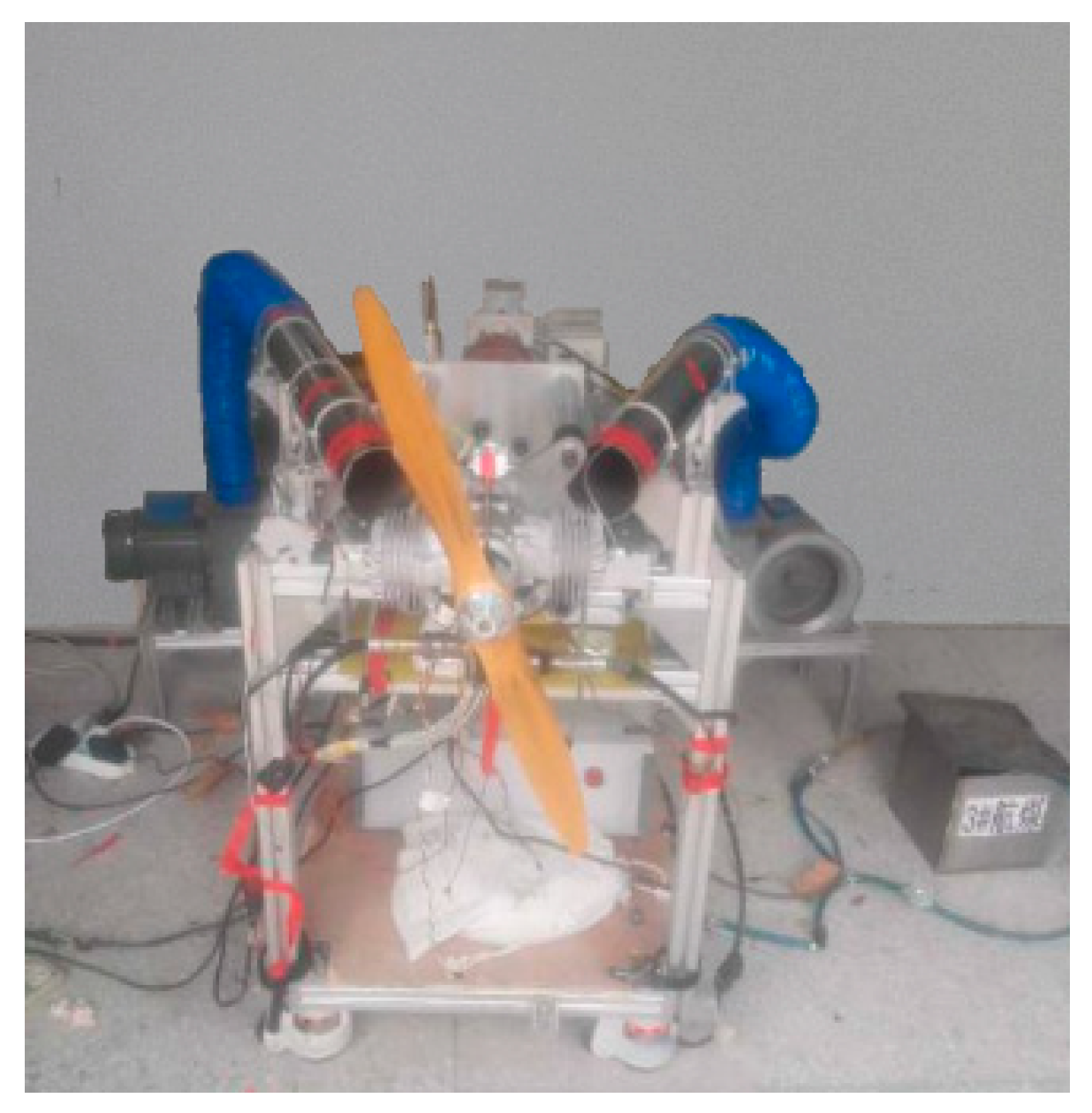
3. Analysis of the Fault State and Establishment of the Fault Data Sample

The content of the fault diagnosis should be clearly defined first before diagnosing the fault. The abnormality of the engine control system mainly includes the fuel injection failure of the injector, low fuel supply pressure, leaks of the exhaust pipe, and the intermittent flameout of engine. Combined with the normal state of the 3 W engine control system, a total of five status types are defined. In this paper, fault injection technology is used to simulate these faults. An engine control system fault diagnosis experimental platform built using various sensors and actuators is shown in Figure 1. With this platform, the fault injection method is used to simulate the control system fault, and the corresponding data is collected and filtered to realize the data sample establishment. In the following analysis process, 80 sets of data are selected from each type of data in the fault sample, among them, 30 sets are used as training sample and 50 sets are used as test sample. All of them make up the data sample.

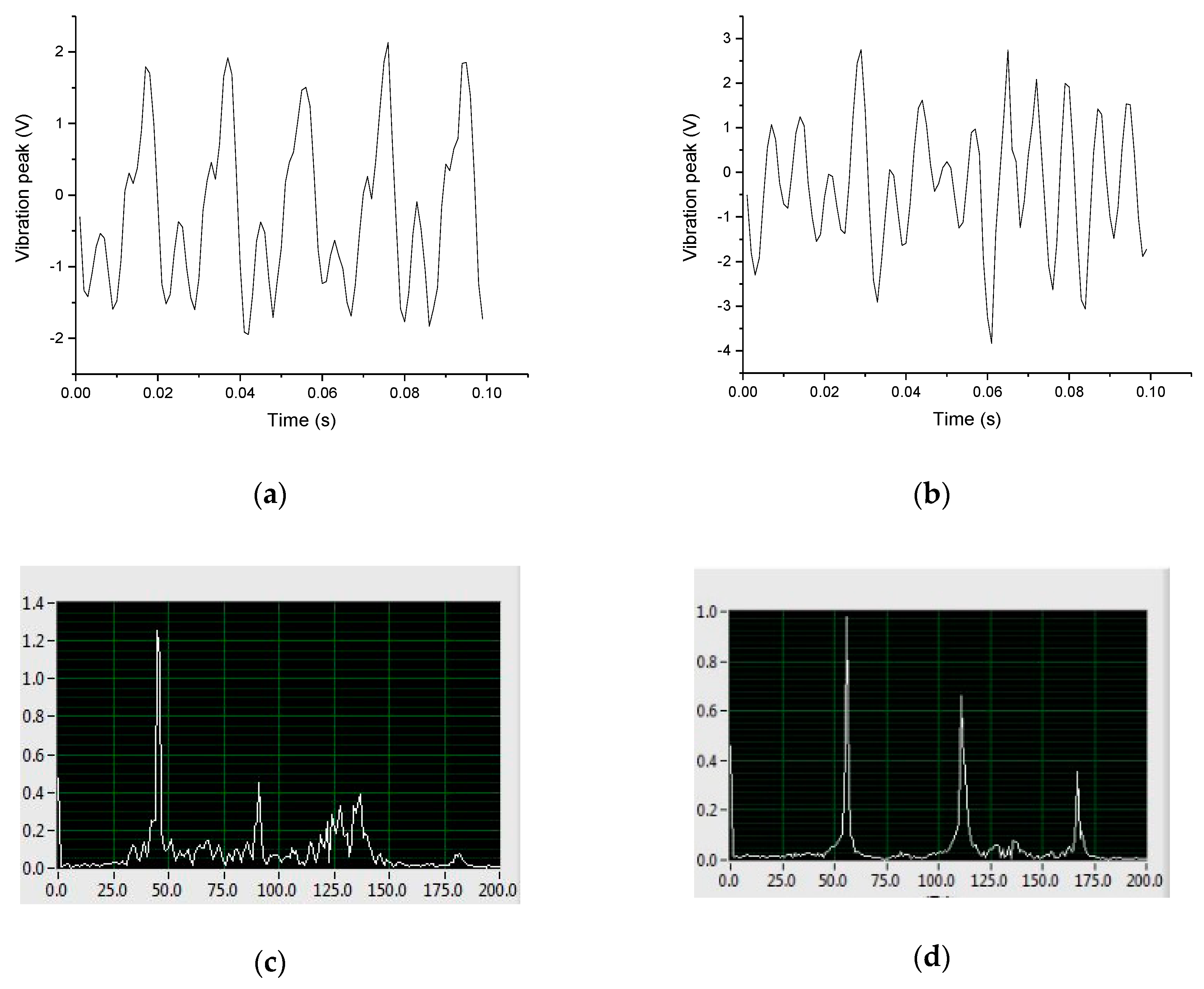
3.1. Analysis of Fault Signal

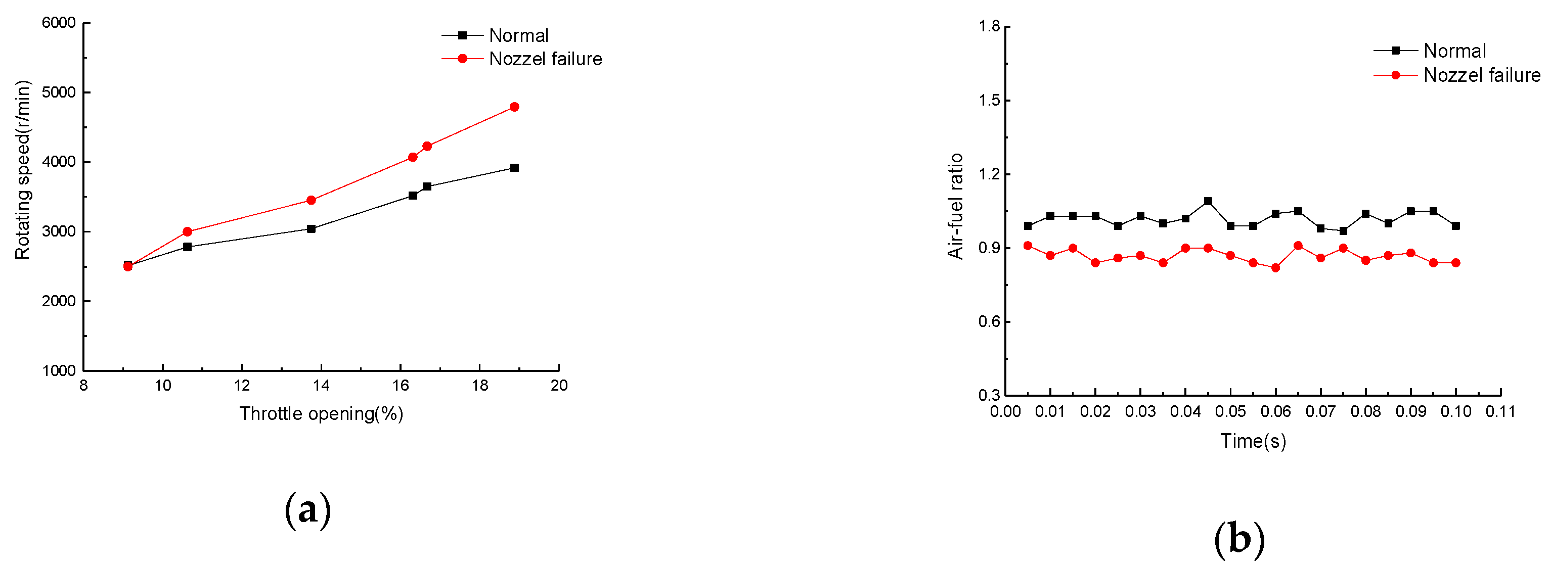
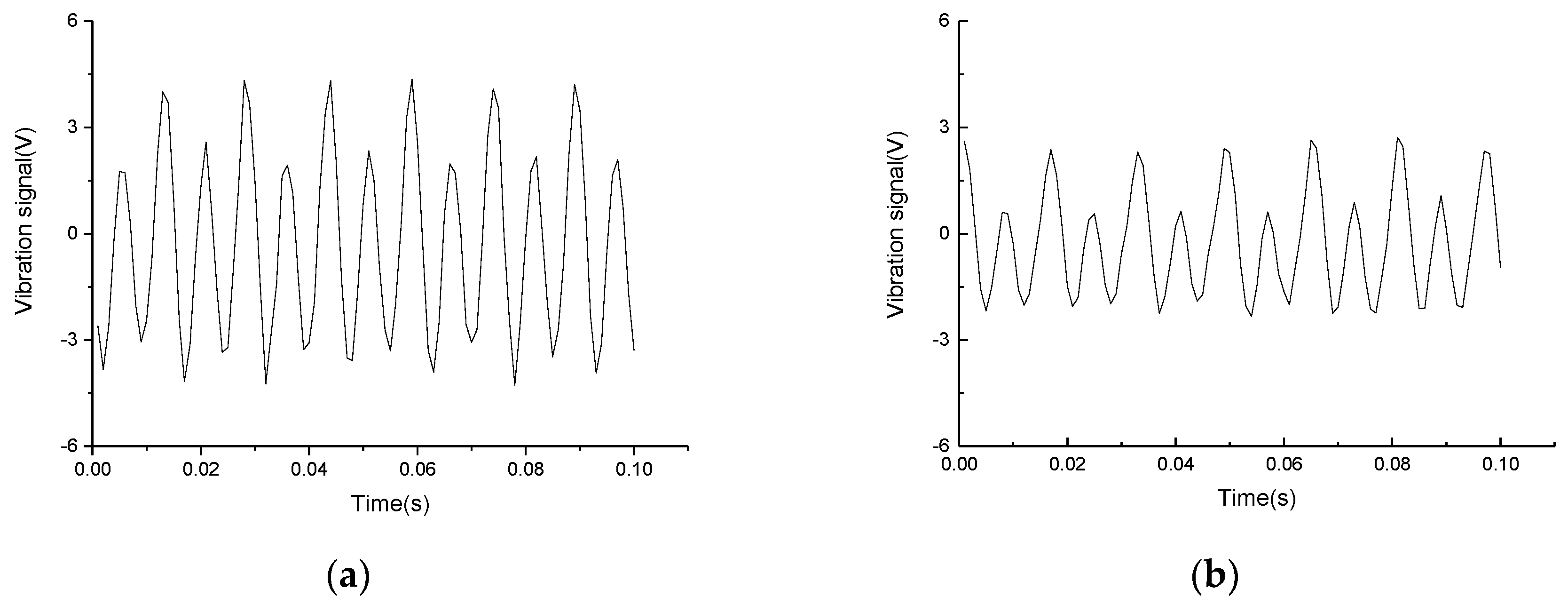
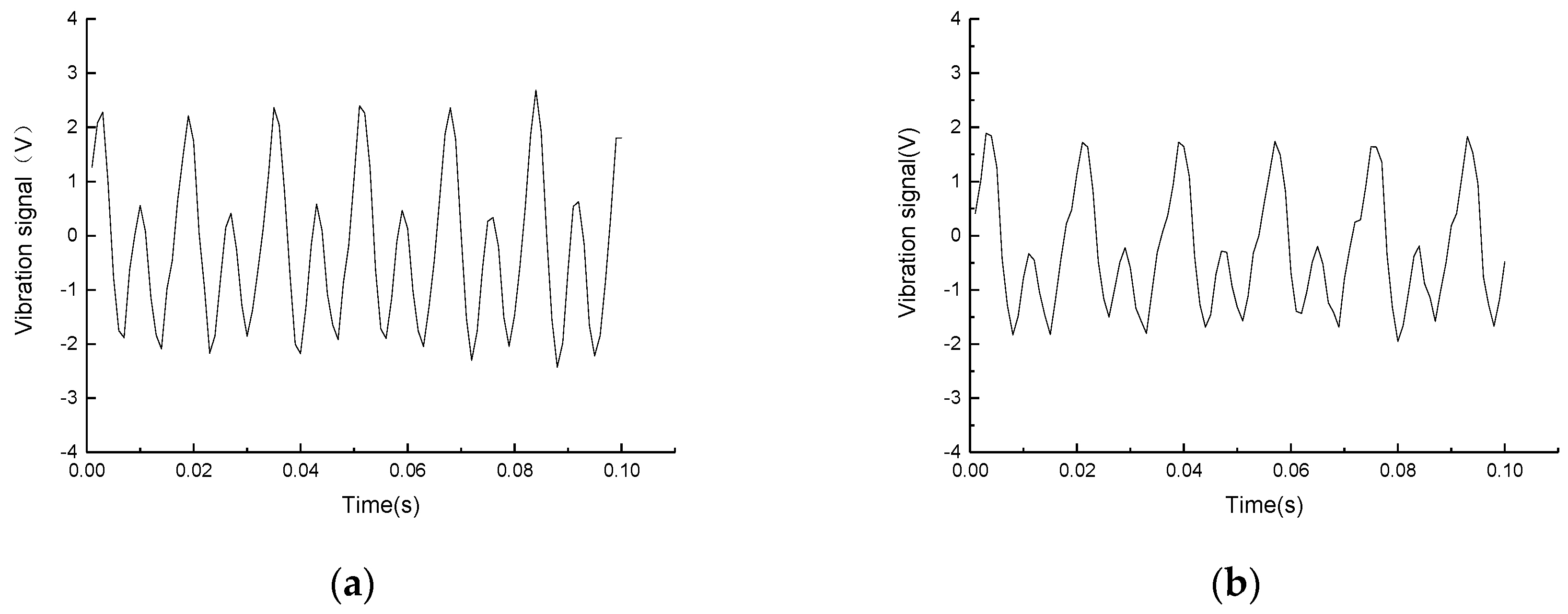
3.1.1. Fuel Injection Failure of the Injector

Fuel injection failure of the injector is mainly achieved by increasing the fuel injection pulse width in the engine fuel injection pulse. When the 3 W engine is working normally, the ECU controls the fuel injection pulse width by querying the engine pulse spectrum data according to the current throttle opening and speed information. When failure occurs, compared with the normal state, the fuel injection pulse width increases, and the fuel injection amount increases. In addition, under the same throttle opening, the engine speed is different when the normal state and the fuel injection pulse width are abnormal. So, the engine speed will increase when the fuel injection amount increases.
Figure 2 shows the change of the speed signal and the air-fuel ratio signal under normal and fuel injection fault conditions. Figure 2a reflects the change of the rotational speed with the throttle opening, the red line represents the change of the rotational speed when the fuel injection fault of the injector occurs, and the black line represents the change of the rotating speed under the normal state. With the figure, it can be gotten that the throttle opening of both is the same at around 2500 r/min. As the throttle opening increases, the difference in the rotational speeds of the two states become larger and larger. Figure 2b reflects the change of the air-fuel ratio of the first cylinder within 0.1 s under the condition of 3500 r/min, wherein the red line represents the air-fuel ratio when the fuel injection is abnormal, and the black line represents the air-fuel ratio under normal conditions. Compared with the two air-fuel ratios, the air-fuel ratio when the fuel injection is abnormal is much smaller than the normal value. This is because the fuel injection amount is too large, causing the incomplete combustion of the fuel which leads to a decrease in the engine air-fuel ratio.
The vibration signal can not only reflect the time domain variation of the engine speed, but the peak value of it can also reflect the amount of function of the engine. At the same rotating speed, the increase of the injection pulse width leads to an increase in the amount of fuel injection, and the engine increases the work per unit time, thus releases more energy. Taking the engine operating at 4000 r/min as an example.
Figure 3 shows the time-domain waveforms of the cylinder vibration under different conditions in 0.1 s. Figure 3a represents the time domain waveform diagram of the cylinder vibration when the fuel injection is abnormal, and Figure 3b represents the cylinder vibration signal in the normal state. As the figure shows, the waveform change law between the two conditions is basically the same, but the peak of the cylinder vibration in the normal state is lower than the peak when the fuel injection is abnormal. This phenomenon further illustrates the energy relationship mentioned above.

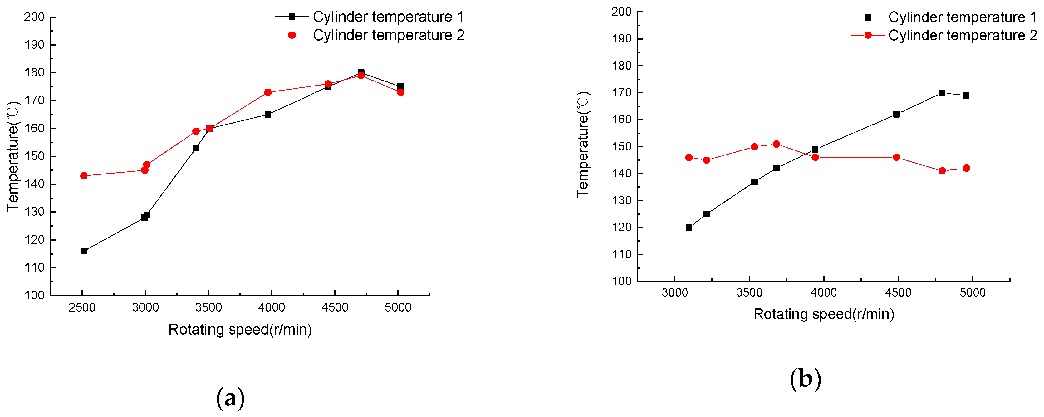
3.1.2. Low Fuel Supply Pressure

The low fuel supply pressure failure is simulated by changing the value of the oil pressure regulating valve. Under normal conditions, the oil pressure of the 3 W engine is 3.0 Bar, and the oil pressure regulator is limited to 2.5 Bar during fault simulation. When the fuel supply pressure is low, it will not only cause the decrease of the unit time power of the engine but also decrease the amount of injected fuel, which will increase the oxygen concentration in the exhaust gas and increase the air-fuel ratio. Since the power is the product of torque and angular velocity, the low fuel supply pressure will also decease the torque when under the same rotation speed.
In addition, low fuel supply pressure will make the engine speed difficult to stabilize. For example, assume that the current engine speed is 4000 r/min, the throttle opening is the same as the normal state. According to the engine pulse spectrum map, the fuel injection pulse width is constant. Since the oil pressure is small, the fuel injection amount is reduced, and the engine speed will be reduced. At this time, compared with the normal state, at the same speed, the throttle opening becomes larger than normal. So, the ECU will increase the injection pulse width. If the influencing factor of the increases of the pulse width is greater than the influence of the oil supply, it will increase the engine speed to about 4000 r/min. The existence of this cycle will make the engine speed difficult to stabilize.
Figure 4 shows the relationship between engine speed and torque under normal conditions and low fuel supply pressure. The black line in Figure 4a represents the speed in the normal state, and the red line represents the speed in the low fuel supply pressure. It can be gotten from Figure 4a that the engine speed is difficult to stabilize when the fuel pressure is too low. Figure 4b represents the relationship between the engine and the torque, where the black line represents the normal data and the red line represents the torque at low fuel pressure. It can be seen that the engine output torque is lower when the fuel pressure is lower at the same speed.
Figure 5 reflects the vibration waveform of the engine at a speed of 3500 r/min. Figure 5a represents the change of the vibration signal with time under normal conditions while Figure 5b represents the change of the vibration signal with time when the fuel pressure is too low. By observing these two figures, it can be seen that under normal conditions, the peak of the vibration signal is greater than 2 V, and when the fuel pressure is too low, the peak of the vibration signal of the cylinder is less than 2 V, which means that when the fuel pressure is too low, the work per unit time is less, and the vibration energy of the engine is smaller.
Figure 6 reflects the changes in engine temperature and speed with normal conditions and low fuel pressure. Figure 6a represents the change of cylinder temperature with the speed under normal conditions. It can be seen from it that when the cylinder is running continuously at a speed of 4500 r/min, the cylinder temperature will exceed 170 degrees, and a fan which uses the PID algorithm to adjust the temperature of the cylinder will be turned on to cool the 3 W engine. With this measure, the temperature of the cylinder will remain around 170 degrees. Figure 6b reflects the situation when the fuel pressure is low. It can be seen from it that the temperature of the number two cylinders is maintained at about 145 degrees with the change of the rotational speed, and the temperature of the number one cylinder will increase and exceed 170 degrees with the increase of the speed. The reason for this may be that the fuel pressure is reduced and the energy released by the combustion of the fuel is reduced, resulting in uneven energy distribution between the two cylinders.

3.1.3. Leaks of the Exhaust Pipe

In this paper, the simulation of the leaks of the exhaust pipe is realized by loosening the connecting bolts between the exhaust pipe of the number two cylinder and the cylinder block. Compared with the normal state, when leaks of the exhaust pipe occur, it will cause a large amount of oxygen to enter the exhaust pipe, which will directly affect the value of the oxygen sensor, thereby increasing the air-fuel ratio. However, leaks of the exhaust pipe have less effect on the engine block vibration, torque, and other signals.
Figure 7 is a comparison diagram of the air-fuel ratio of the two cylinders under normal conditions and when the number two-cylinder exhaust pipe leaks. Figure 7a represents the relationship between the air-fuel ratio and the rotational speed, and Figure 7b shows the change of the air-fuel ratio within 0.1 s in the engine at 3000 r/min, where the black line represents the air-fuel ratio of the number two cylinder in the normal state, and the red line represents the air-fuel ratio when the exhaust pipe leaks. It can be seen from the figure that whether in the time domain or in the frequency domain, the leaks of the exhaust pipe will cause the air-fuel ratio to increase compared with the normal state.

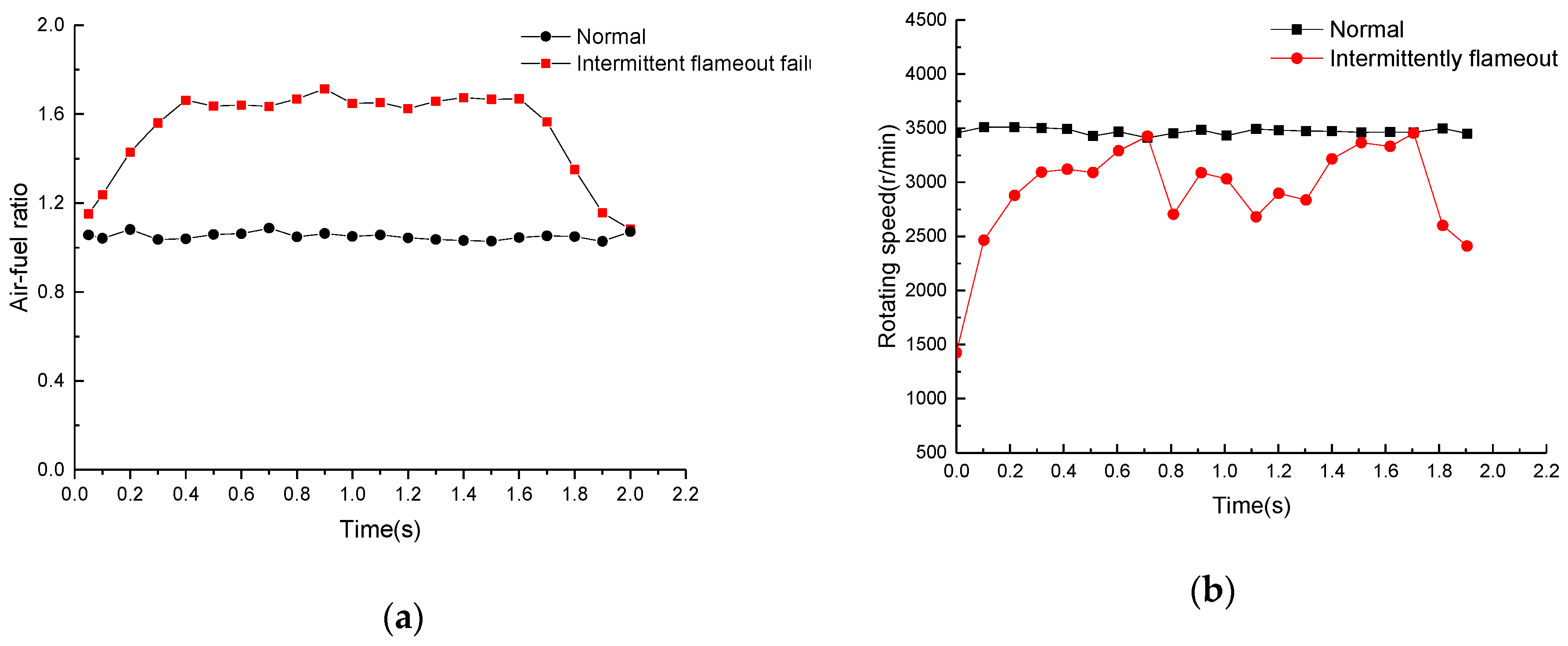
3.1.4. The Intermittently Flameout of Engine

The intermittent flameout of engine is simulated by continuously turning off the power supply of the igniter. In theory, the ECU will continue to inject the fuel when the engine is not ignited. At this time, the fuel cannot be burned, the oxygen concentration in the exhaust gas is reduced, and the air-fuel ratio signal is reduced. However, the ECU of the 3 W engine used in this platform receives the speed signal from the igniter, so once the igniter is de-energized, the ECU cannot find the speed signal, and the fuel injection pulse width will not be generated, resulting in the failure to inject oil. The air-fuel ratio will increase sharply compared to normal state.
Figure 8a reflects the change of air-fuel ratio with time, in which the black line and the red line represent the air-fuel ratio under normal state and the air-fuel ratio under intermittent flameout failure state, respectively. It can be seen from the figure that at the moment when the ignition is turned off, the air-fuel ratio will gradually increase due to the loss of the injection pulse width. As the engine starts, the air-fuel ratio will gradually return to normal. Also, the rotating speed of the engine will be decreased sharply when the ignition is turned off and return to normal as the engine starts. However, it should be noticed that at the moment of restart, the engine’s speed fluctuates greatly. Figure 8b represents the change of the speed with time in the two states of the engine at 3500 r/min.
The intermittent flameout of engine will cause the harmonic component of the engine vibration signal to increase. Figure 9 shows the frequency and time domain of the vibration signal under normal engine conditions and intermittent flameout failures. Among them, Figure 9a,c represents the time domain and the frequency domain waveform diagrams of the vibration signal under normal state. While Figure 9b,d represent the time domain and the frequency domain waveform diagrams of the vibration signal under intermittent flameout failure state. Through the comparison of the four images, it can be found that the waveform of the vibration signal is very irregular under the intermittent flameout state, and the acquired time-domain waveform contains a large number of irregular harmonics.

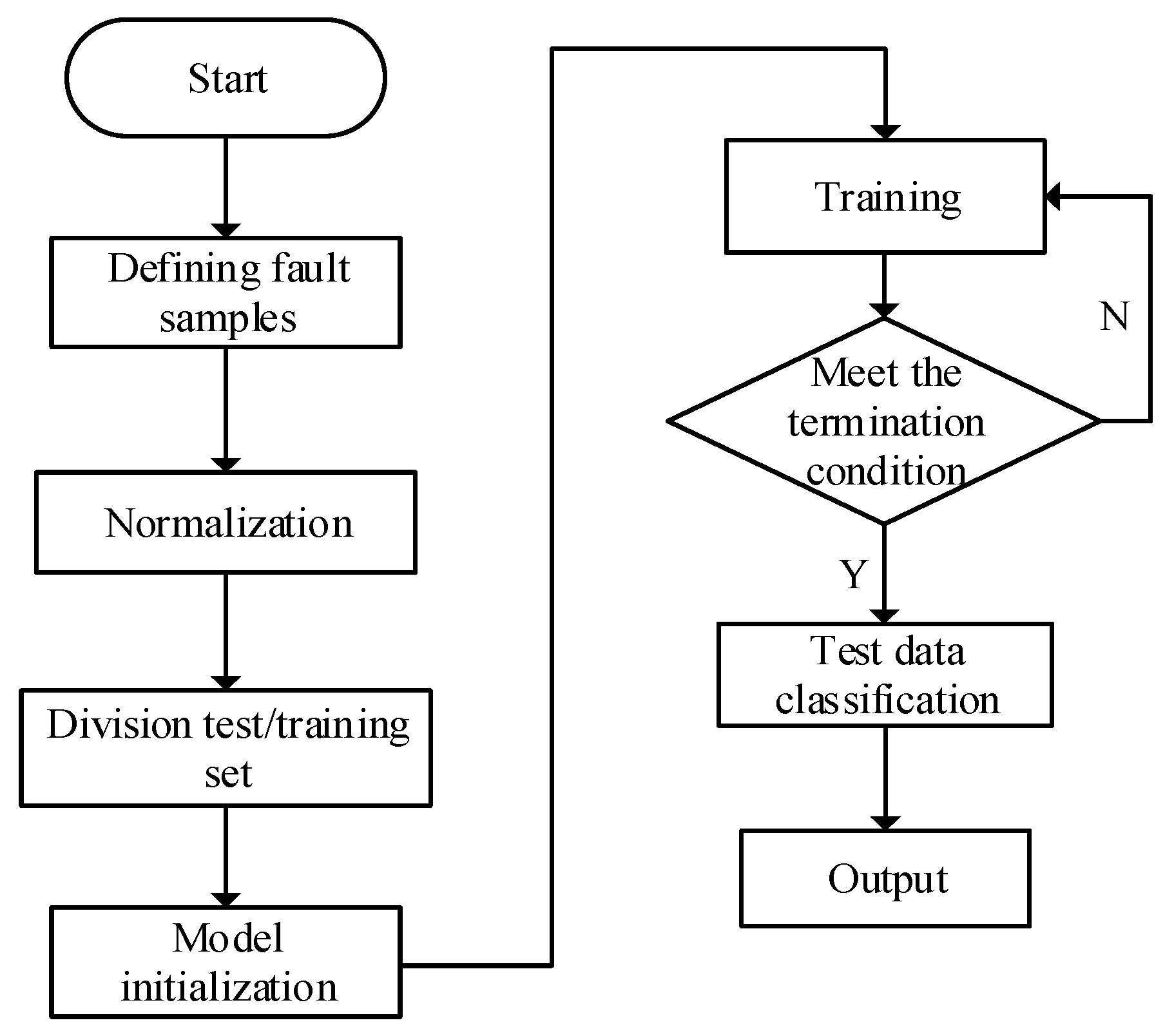
3.2. Creation of the Fault Diagnosis Data Sample

According to the analysis results of the characteristic signals in each fault state in Section 3.1, it is found that the characteristic signal can establish a single mapping relationship with each fault sample. The correspondence between fault characteristics and characteristic signals is shown in Table 1.
Data samples for fault diagnosis is established by finding analog signals such as vibration signals in the frequency domain of the corresponding speed. The 8-dimensional vectors ( x 1 , x 2 , x 3 , x 4 , x 5 , x 6 , x 7 , x 8 ) . are used as inputs to probabilistic neural networks and support vector machines. Among them, x 1 represents the current rotating speed, x 2 represents the throttle opening, x 3 represents the frequency signal, x 4 represents the vibration peak, x 5 and x 6 represent temperatures of the two cylinders, x 7 and x 8 represent the two-cylinder air-fuel ratios, respectively. During the experiment, the rotating speed was within 2500–5500 r/min, and the rotating speed was increased at 500 r/min intervals. In each fault state, 80 sets of data were recorded and screened out. The data of each state is collected as data samples, and some typical data of each fault state with an engine speed of about 3000 r/min are shown in Table 2.
The status bar in the table indicates the state of the engine control system, state 1 represents the engine control system is normal, state 2 represents the fuel injection failure of the injector, state 3 represents the low fuel supply pressure, state 4 represents the leaks of the exhaust pipe, and state 5 represents the intermittent flameout of engine. With the data shown in Table 2, it can be seen that when an injector failure occurs, the throttle increases due to an increase in the amount of fuel injection, the air-fuel ratio of the two cylinders increases, and the vibration peak increases, which is consistent with the actual situation. When the fuel pressure is too low, due to the decrease of the fuel supply amount, the throttle opening increases, the vibration peak decreases, and the air-fuel ratio of the two cylinders increase at the same rotation speed, which is also consistent with the actual situation. Similarly, when the number 2-cylinder exhaust pipe leaks, the air-fuel ratio of the number 2 cylinder increases due to air leakage from the exhaust pipe, which is also consistent with the actual situation. In the state where the engine is intermittently flameout, since the injector of the 3 W engine does not inject fuel, the air-fuel ratio of the two cylinders increases compared with the normal condition, which is consistent with the actual situation. Therefore, a conclusion can be gotten that all the fault states’ data filtered by the fault sample are truly valid.

3.3. Data Processing

After the sample data is acquired, the fault diagnosis algorithms chosen before are used to sort the data. The specific processing of the two algorithms can be shown with the following flowchart which named with Figure 10.
Firstly, the data sample should be defined with different kinds which are shown in Table 2. After that, due to the different units of the signals, the accuracy of the data classification may be reduced. So, the normalization of the sample is used here. The form is shown with Equation (10).
f : x i y i = ( y i max y i min ) x i x i min x i max x i min + y i min
where x i represents the value of each element in the input vector, y i represents the normalized value. x i max and x i min represent the maximum and minimum values of the same type of elements in the input vector respectively, and setting the value of the output between 1 and −1, which means the y i max = 1 and   y i min = 1 .

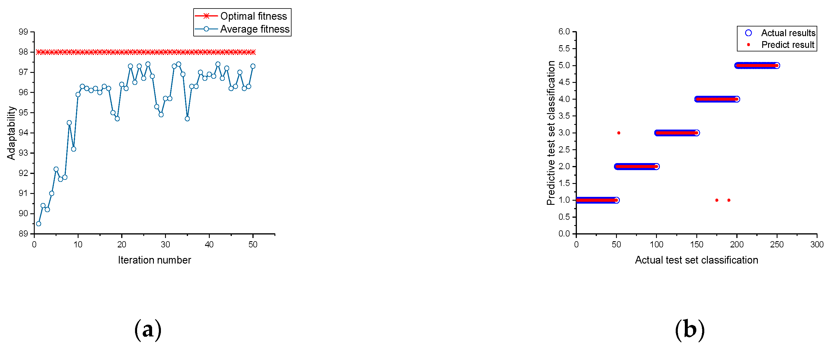
4. Introduction to Particle Swarm Optimization Algorithm

Particle Swarm Optimization is a kind of optimization algorithm based on swarm intelligence. Compared with the genetic algorithm, PSO has no process of selection, crossover and mutation, and the optimization process is relatively simple [21].
The PSO algorithm requires that a group of random particles be initialized first in a certain spatial range, and then the particles follow the current optimal particle and begin to iteratively search for the optimal solution in space. The number of iterations depends mainly on the number of populations [22]. Assuming that in a D-dimensional search space, the position and velocity of the i-th particle are x i = [ x i 1 , x i 2 , x i D ] and V i = [ V i 1 , V i 2 , , V i D ] . In each iteration, the particle finds the optimal solution of the individual p i = [ p i 1 , p i 2 , p i D ] and the optimal solution in the population p g = [ p g 1 , p g 2 , p g D ] . Then the current speed and location are updated through Equations (11) and (12).
v i j ( k + 1 ) = w v i j + c 1 r 1 [ p i j x i j ( k ) ] + c 2 r 2 [ p g j x i j ( k ) ]
x i j ( k + 1 ) = x i j ( k ) + v i j ( k + 1 ) , j = 1 , 2 D
where w = 1 represents the inertia weight, c 1 = 1.5 and c 2 = 1.7 represent the learning factor, r 1 and r 2 represent the random number between 0 and 1.
Due to the optimization goal is to optimize the accuracy of algorithm classification, which is a single optimization target, the basic particle swarm optimization which uses a single objective optimization function is used in this paper. The specific form of the optimization function is given in the specific analysis below.

5. Results and Analysis of the Optimization Algorithm

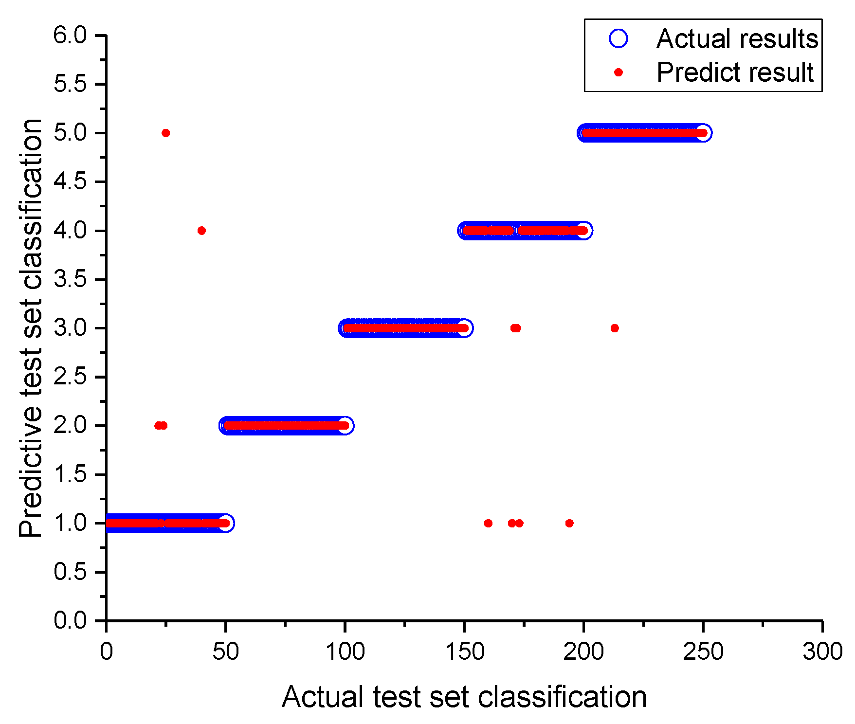
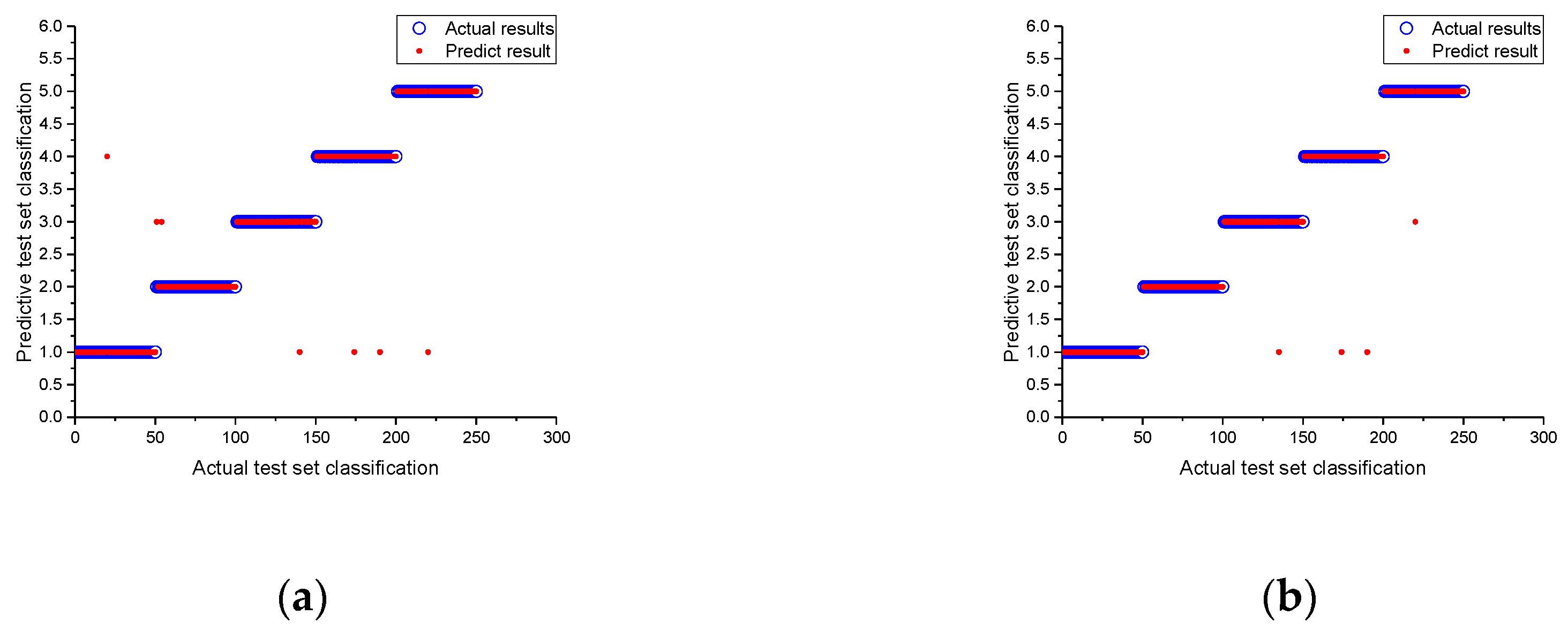
5.1. Results of the Probabilistic Neural Optimization

According to the sample screening results, the constituent eigenvectors of the eight characteristic signals are used as the input vectors of the probabilistic neural network.
In Figure 11, the red dot represents the result of the probabilistic neural network for each input vector classification prediction, while the blue circle represents the actual data result. When the red dot coincides with the blue circle, the classification can be regarded as correct. It can be seen from the figure that when under the normal state, the exhaust pipe leakage state and the intermittent flameout of engine state, some sample points are misclassified, while under the other states, the classification result is completely correct. By statistically correcting the classification prediction results, the classification results of the probabilistic neural network are obtained. The value of σ can affect the accuracy of the classification. When the smoothing factor σ = 0.5, the classification accuracy of the whole test sample is as high as 92.8%, and the result is ideal. On the one hand, the high accuracy rate proves the excellent classification characteristics of the probabilistic neural network. On the other hand, it also reflects that the screening of characteristic signals and the establishment of fault data samples are accurate.
The process of PSO optimization probabilistic neural network is based on training samples, through the idea of cross-validation to find the optimal smoothing factor. The cross-validation ideal means to group the original data, one part as a test set and the other part as a verification set, and using the training set to train the classifier firstly, then using the verification set to test the trained model to obtain the classification accuracy as a performance indicator for evaluating classifiers. The basic mathematical relationship of the objective function in a probabilistic neural network can be expressed as Equation (13).
v a l u e = f ( σ )
In the objective function, σ is the input variable, and value represents fitness. The actual meaning of value is the average classification accuracy under cross-validation. The purpose of optimization is to find the maximum fitness value in the optimization process and the corresponding σ.
In the PNN network, the optimization process is relatively simple because only one parameter σ needs to be changed. Set the value of σ to [0.01, 1]. The maximum evolution number of the population in the particle swarm is 50, and the population number is 20. The iterative optimization process and the final classification result are shown in Figure 12. After solving, the probability of a probabilistic neural network is the highest when σ = 0.1803 and finally reaches 96.4%. The error rate that still exists may be caused by the unclassifiable samples.

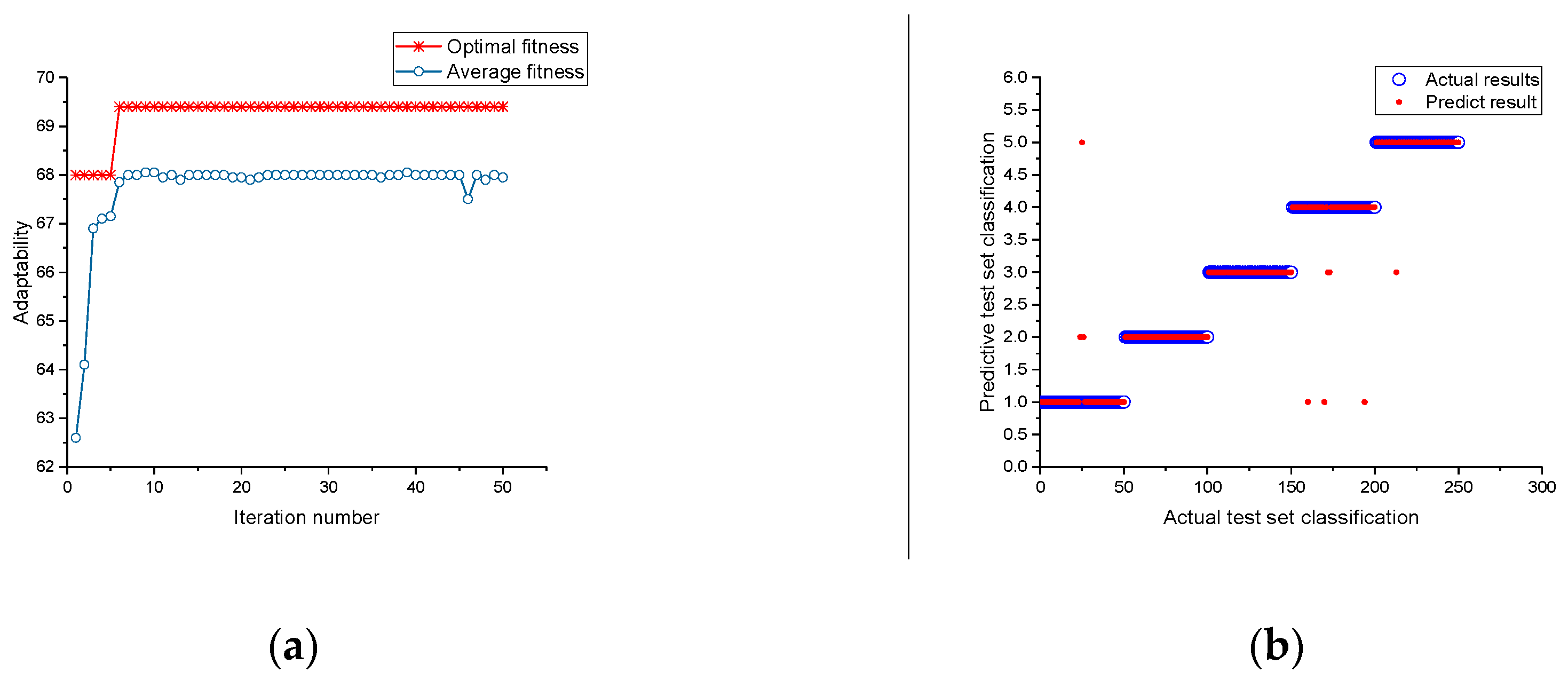
5.2. Results of the Support Vector Machine Optimization

The kernel functions of SVM are various. The different kernel functions are selected to observe the influence of the kernel function on the final classification result. The support vector machine inputs the feature vectors composed of 8 feature signals, and the output is the classification prediction result for each feature vector.
Figure 13 shows the results of different kernel function data classification. Figure 13a–d represent the classification results using linear kernel functions, radial basis kernel functions, polynomial kernel functions, and Sigmoid kernel functions, respectively. The blue circle in the figures represents the actual label of the sample, and the red dot represents the label of the SVM classification prediction. The higher the coincidence of the red dot and the blue circle, the higher the accuracy of the classification. Table 3 represents the final classification results of the test samples when different kernel functions are used when selecting C-SVM in SVM. Since there is no clear chosen principle for the penalty parameter c and the kernel function parameter g, c = 2 and g = 1 are randomly selected here. The results in Table 3 show that under the condition of this parameter, among the four kernel functions, the polynomial kernel function has the highest classification accuracy, and the Sigmoid kernel function has the lowest classification accuracy.
When using the PSO algorithm to optimize the SVM algorithm, taking C-SVM as an example, firstly the appropriate range of c and g values should be chosen. Then based on the training samples, the cross-validation method is used to output the average classification accuracy under cross-validation of training samples. After multiple iterations of PSO, finding the best average classification accuracy and the best c, g parameters of the training samples. Finally, using the best c and g parameters to complete the classification of the test samples. Through this way, the classification accuracy can be improved and the generalization ability of the classifier under the parameter state can be judged. Taking the Sigmoid kernel function as an example to introduce the optimization process of PSO. The basic mathematical relationship of the objective function in this optimization is shown with Equation (14).
v a l u e = f ( c , g )
In this equation, the penalty parameter c and the kernel function parameter g are input variables, and the value represents the fitness of the particle swarm algorithm in the equation, which actually represents the classification accuracy of SVM. By inputting different c and g parameters during the optimization process, the maximum fitness can be found.
Figure 14 represents the iterative optimization process of the Sigmoid kernel function in SVM and the final classification effect on the test samples. The fitness of Figure 14a represents the accuracy of the actual classification. The average fitness is the average of the accuracy of all particle classifications in a single solution, the best fitness is the highest accuracy of particle classification in an iterative process. In the optimization process, the value of the penalty factor c is set to (22, 28), and the value of the kernel function parameter g is set to (2−8, 2−2). After several iterations, the Sigmoid kernel function finds the best c and g parameters. The classification of the test samples was re-completed using the c and g parameters, and the final accuracy was actually as high as 98.8%. The final classification effect is shown with Figure 14b. The high accuracy indicates that Sigmoid does have good and generalization ability in the range of values of c and g. On the other hand, it also shows that the range of values of c and g is relatively correct.

5.3. Comparison and Analysis of Diagnostic Method Results

It can be seen from Table 4 that PNN and SVM are found to have high classification accuracy when dealing with engine fault data, indicating the correctness of the selection of these two intelligent algorithms and feature signal data samples. Through the optimization of the PSO algorithm, the classification accuracy of Sigmoid kernel function in SVM is greatly improved. The classification results of kernel function and PNN in SVM have improved. On the one hand, the importance of the range of parameter values is explained. On the other hand, it also shows that PSO has optimize the important parameters that affect the classification results. Overall, compared to PNN, after being optimized by PSO, SVM classification accuracy is higher, reflecting the advantages of SVM in small sample data classification. In the SVM classification, the polynomial kernel function of v-SVM and the Sigmoid kernel function in C-SVM have the highest classification accuracy. From the perspective of the whole optimization process, the SVM parameters are relatively numerous. It is difficult to select the penalty parameter c and the kernel function parameter g. However, unlike SVM, PNN only needs to set the smoothing factor σ, so the optimization process is relatively simple, and compared with SVM, PNN is more convenient to use.

6. Conclusions

In this paper, a fault diagnosis and optimization method for engine control system based on probabilistic neural network and support vector machine are proposed. The German 3 W piston engine is used as a control object, and the fault injection method is used to cause failures of the engine control system. The mapping relationship between the characteristic signal and various faults is established according to the data characteristics of the feature signal. Then, by doing experiments, the engine fault diagnosis data samples are established. After that, the particle swarm optimization algorithm is used to optimize the important parameters of the probabilistic neural network and the support vector machine. By analyzing and comparing the results of fault diagnosis, it shows that the fault diagnosis method based on probabilistic neural network and support vector machine can effectively diagnose the common faults of the control system. Under the optimization of particle swarm optimization algorithm, the accuracy of PNN and SVM fault diagnosis classification results are significantly improved. The classification accuracy of PNN is up to 96.4%, and the classification accuracy of SVM is up to 98.8%, which greatly improved the applicability of PNN and SVM in fault diagnosis technology of aviation piston engine control system.

Author Contributions

Writing—original draft preparation, B.W.; writing—review and editing, H.K.; data curation, X.M.; project administration, B.Y.

Funding

This work is supported by the Fundamental Research Funds for the Central Universities (grant no. NS2018017).

Conflicts of Interest

The authors declare no conflict of interest.

References

  1. Barrett, W.J.; Rembold, J.P.; Burcham, F.W. Flight test of a full authority Digital Electronic Engine Control system in an F-15 aircraft. AIAA J. 1981. [Google Scholar] [CrossRef]
  2. Chen, Q. Some measures to improve engine reliability. Civ. Aviat. Technol. 2002, 1, 39–41. [Google Scholar]
  3. Yan, J. Research on Fault Diagnosis Expert System of Aviation Piston Engine Based on Fault Tree Analysis. Ph.D. Thesis, University of Electronic Science and Technology of China, Chengdu, China, 2010. [Google Scholar] [CrossRef]
  4. Akhenak, A.; Chadli, M.; Maquin, D.; Ragot, J. Sliding mode multiple observer for fault detection and isolation. In Proceedings of the 42nd IEEE International Conference on Decision and Control, Maui, HI, USA, 9–12 December 2003. [Google Scholar] [CrossRef]
  5. Jiang, B.; Staroswiecki, M.; Cocquempot, V. Fault Accommodation for Nonlinear Dynamic Systems. IEEE Trans. Autom. Control 2006, 51, 1578–1583. [Google Scholar] [CrossRef]
  6. Jiang, B.; Gao, Z.; Shi, P.; Xu, Y. Adaptive Fault-Tolerant Tracking Control of Near-Space Vehicle Using Takagi–Sugeno Fuzzy Models. IEEE Trans. Fuzzy Syst. 2010, 18, 1000–1007. [Google Scholar] [CrossRef]
  7. Chadli, M.; Davoodi, M.; Meskin, N. Distributed state estimation, fault detection and isolation filter design for heterogeneous multi-agent linear parameter-varying systems. IET Control Theory Appl. 2017, 11, 254–262. [Google Scholar] [CrossRef]
  8. Sebastiani, F. Machine learning in automated text categorization. ACM Comput. Surv. 2002, 34, 1–47. [Google Scholar] [CrossRef]
  9. Ye, Z.; Sun, J. Probabilistic neural networks based engine fault diagnosis. Acta Aeronaut. Astronaut. Sin. 2002, 23, 155–157. [Google Scholar] [CrossRef]
  10. Bedekar, P.P.; Bhide, S.R.; Kale, V.S. Fault section estimation in power system using Hebb’s rule and continuous genetic algorithm. Int. J. Electr. Power Energy Syst. 2011, 33, 457–465. [Google Scholar] [CrossRef]
  11. Ni, J. Reasearch on Fault Diagnosis and Hardware-in-loop Simulation for Actuator of Aero-Engine. Ph.D. Thesis, Nanjing University of Aeronautics and Astronautics, Nanjing, China, 2016. [Google Scholar]
  12. Ding, L. Engine Fault Diagnosis Based on IMF Band Energy Characteristics and Support Vector Machine. Intern. Combust. Engines Fitt. 2018, 5, 105–107. [Google Scholar]
  13. Dai, Y.; Wang, J.; Liu, G. Optimum Decoder for Barni’s Multiplicative Watermarking Based on Minimum Bayesian Risk Criterion. In Proceedings of the 2008 IEEE International Conference on Networking, Sensing and Control, Sanya, China, 6–8 April 2008 . [Google Scholar] [CrossRef]
  14. Lu, Y. Stock Market Trend Forcast Based on Parameter Optimized Support Vector Model. Ph.D. Thesis, Zhejiang Gongshang University, Hangzhou, China, 2013. [Google Scholar] [CrossRef]
  15. Wang, F. Research and Application of Support Vector Machine Algorithm. Ph.D. Thesis, Jiangnan University, Wuxi, China, 2008. [Google Scholar]
  16. Vapnik, V.N. The Nature of Statistical Learning Theory; Springer Science & Business Media: Berlin, Germany, 1995. [Google Scholar] [CrossRef]
  17. Chen, G. Bayesian layered model based on MCMC simulation and its application. Sci. Technol. J. Electron. Ed. 2015, 4, 76–77. [Google Scholar] [CrossRef]
  18. Chen, M. Principles and Examples of MATLAB Neural Network; Tsinghua University Press: Beijing, China, 2013. [Google Scholar]
  19. Chen, Y.; Xiong, Q. Support Vector Machine method Application Tutorial; Meteorological Press: Beijing, China, 2011. [Google Scholar]
  20. Yang, X.; Hao, Z. Algorithm Design and Analysis of Support Vector Machine; Science Press: Beijing, China, 2013. [Google Scholar]
  21. Gong, C.; Wang, Z. Proficient in MATLAB Optimization Calculation; Publishing House of Electronics Industry: Beijing, China, 2014. [Google Scholar]
  22. Xu, J.; Li, Z.; Wang, H.; Qian, F. A new particle swarm optimization for multiobjective problem. Comput. Digit. Eng. 2006, 34, 31–34. [Google Scholar] [CrossRef]
Figure 1. Fault diagnosis test platform for the engine control system.
Applsci 09 04122 g001
Figure 2. Change chart of speed and air-fuel ratio under normal and nozzle failure conditions. (a) Chart of speed variation with throttle opening, (b) Chart of transient air-fuel ratio change with different air-fuel ratios.
Applsci 09 04122 g002
Figure 3. Vibration waveform of nozzle failure and normal condition. (a) Nozzle fault vibration waveform, (b) Normal vibration waveform.
Applsci 09 04122 g003
Figure 4. Rotating speed and torque change diagram. (a) Curve of rotating speed varying with time, (b) Curve of torque varying with time.
Applsci 09 04122 g004
Figure 5. Vibration signal waveform under low oil pressure and normal conditions. (a) Vibration waveform in the normal state, (b) Vibration waveform when fuel pressure is low.
Applsci 09 04122 g005
Figure 6. Temperature change chart of two cylinders under normal condition and low fuel pressure condition. (a) Change chart of cylinder temperature in normal condition, (b) Change chart of cylinder temperature when fuel pressure is low.
Applsci 09 04122 g006
Figure 7. Air-fuel ratio diagram of exhaust pipe leakage and normal conditions. (a) Chart of air-fuel ratio changing with rotating speed, (b) Change chart of transient air-fuel ratio.
Applsci 09 04122 g007
Figure 8. Charts of speed and air-fuel ratio changing with time. (a) Chart of air-fuel ratio versus time, (b) Change chart of transient speed.
Applsci 09 04122 g008
Figure 9. Time-domain and frequency-domain analysis chart of vibration signals. (a) Vibration waveform in normal state, (b) Vibration waveform of flameout fault, (c) Frequency domain diagram of normal state, (d) Frequency domain diagram of flameout fault.
Applsci 09 04122 g009
Figure 10. Flowchart of the program.
Applsci 09 04122 g010
Figure 11. Classification results of PNN.
Applsci 09 04122 g011
Figure 12. PNN iterative process and results after PSO optimization. (a) Iterative optimization process, (b) Final classification results.
Applsci 09 04122 g012
Figure 13. Classification results of SVM kernel function. (a) Linear kernel function, (b) Polynomial kernel function, (c) Radial basis function, (d) Sigmoid kernel function.
Applsci 09 04122 g013aApplsci 09 04122 g013b
Figure 14. PSO iterative optimization and final results. (a) Iterative optimization process, (b) Final classification results.
Applsci 09 04122 g014
Table 1. Mapping relationship between fault types and characteristic signals.
Fault TypeThe Signature Signals Required for Establishing the Mapping
The fuel injection failure of the injectorThrottle opening, air-fuel ratio signal and vibration peak
Low fuel supply pressureRotating speed signal, vibration peak, air-fuel ratio signal, throttle opening, torque signal and cylinder temperature signal
Leaks of the exhaust pipeAir-fuel ratio signal
The intermittent flameout of engineAir-fuel ratio signal, rotating speed signal and vibration frequency domain signal
Table 2. Fault sample data.
Rotating Speed (r/min)Throttle Opening (%)Vibration Frequency (Hz)Vibration Peak Value (V)Cylinder Temperature of Number 1 (°C)Cylinder Temperature of Number 2 (°C)Number One Cylinder λNumber Two-Cylinder λState
353916.563592.301581590.981.021
350814.813592.821591580.910.932
349417.813581.951381511.131.263
357516.813582.281571591.311.034
346116.875592.231581571.201.235
Table 3. Results analysis of different kernel functions in C-SVM.
Kernel FunctionAccuracySVM Train Parameter Options
Linear kernel function96.4%c = 2, g = 1, t = 0
Polynomial kernel function98.4%c = 2, g = 1, t = 1
Radial basis kernel function93.6%c = 2, g = 1, t = 2
Sigmoid kernel function40.4%c = 2, g = 1, t = 3
Table 4. Comparison of PNN/SVM classification results.
Classification ModelClassification Accuracy (%)Optimized Accuracy with PSO (%)
Probabilistic neural network92.896.4
C/v-SVM linear kernel function96.4/96.497.6/98.4
C/v-SVM polynomial kernel function98.4/84.498.4/98.8
C/v-SVM radial basis kernel function93.6/99.299.2/96.8
C/v-SVM Sigmoid kernel function40.4/87.698.8/92.4

