1. Introduction
Multi-agent path planning (MAPP) involves finding the set of least-cost paths for a set of agents co-existing in a given
graph such that each of the agents is free from collision, where a collision is defined as at least two agents moving to the same location at the same time. MAPP attracts increasing attention due to its practical applications in multi-robot systems for surveillance automation, video gaming, traffic control, and many other domains [
1,
2,
3,
4]. This problem is, however, difficult to solve because the configuration space grows exponentially with the number of agents in the system, incurring extremely heavy computational efforts. It is an NP-hard problem to find optimal solutions for MAPP in its general form [
5].
Approaches to solving MAPP problems fold into three main categories:
coupled, decoupled and
intermediate [
6].
Coupled approaches search the
joint configuration space of the multi-agent system, which is the
Tensor product of the free configuration spaces of all the individual agents. A popular coupled planner is the A* algorithm [
7] that directly searches the whole joint configuration space, making such an approach computationally infeasible when the number of agents is large. Enhanced variants of A*, such as operator decomposition (OD), enhanced partial expansion A* (EPEA*), and iterative deepening A* (IDA*), can—to some extent—mitigate the exponential growth in the number of neighbors by improving the admissible heuristics [
8,
9,
10,
11]. Coupled approaches are optimal and complete, but usually at high computational cost.
Decoupled approaches plan for each agent separately and then adjust the path to avoid collisions. Algorithms in this category are generally faster because they perform a graph search and collision-avoidance adjustment in low-dimensional spaces. However, optimality and completeness are not guaranteed [
3,
12].
Intermediate approaches lie between coupled and decoupled ones because they dynamically couple agents and grow the search space during the planning. In this way, the search space is initially small and grows when necessary. A few intermediate MAPP algorithms can guarantee optimality and completeness. State-of-the-art examples include Conflict-Based Search (CBS) [
6,
13]. CBS is a two-level algorithm. At the high level, conflicts are added into a
conflict tree (CT). At the low level, solutions consistent with the constraints given by the CT are found and updated to agents. CBS behaves poorly when a set of agents is strongly coupled. Meta-agent CBS (MA-CBS) is then proposed by merging strongly coupled agents into a meta-agent to handle the strongly coupled scenarios.
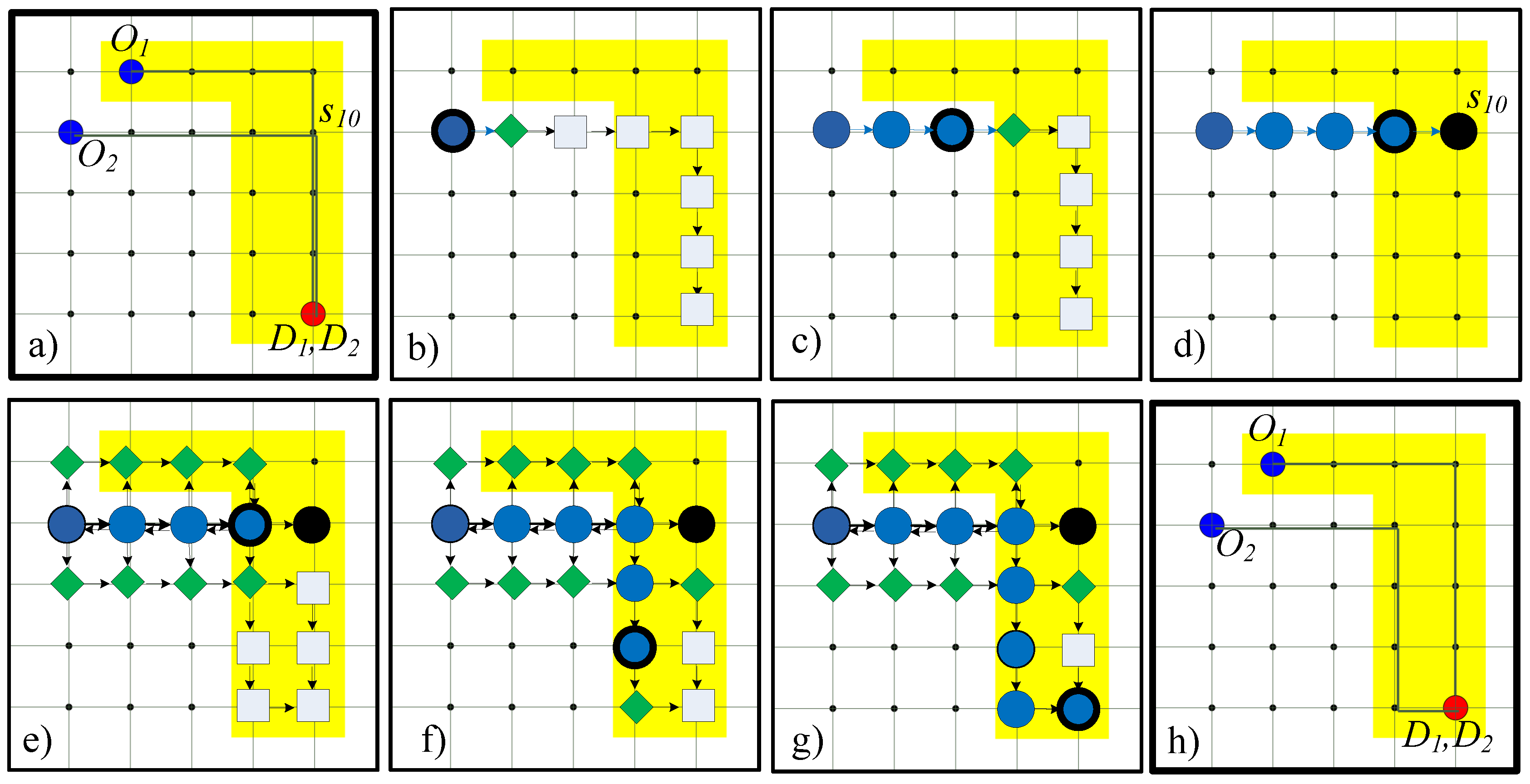
The M* algorithm is a state-of-the-art coupled approach. It starts with decoupled planning and applies a strategy called
sub-dimensional expansion to dynamically increase the dimensionality of the search space in regions in which agent collisions occur. In this way, an efficient graph search with a strict collision-free constraint can be achieved, while minimizing the explored portion of the joint configuration space. M* identifies which subsets of agents can be safely decoupled and hence plans for multi-agents in a lower-dimensional space. Compared to CBS and its variant MA-CBS, M* and its variants, e.g., recursive M* (rM*), have much more fine-grained control over some technical details, such as the management of conflict sets for better scalability. The fine-grained nature of M* allows it to be integrated into MA-CBS to take advantage of both [
14]. Recent work extended both M* and CBS algorithms to handle the imperfect path execution due to unmodeled environments and delays [
15,
16].
Most fundamental MAPP approaches assume hard collisions, which means that solutions in which agents share resources (nodes or edges) are rejected. In many real world scenarios, some degree of resource sharing between agents is acceptable, so the hard-collision constraint needlessly over-constrains the solution space. This paper relaxes the hard collisions constraint by allowing some sharing of resources, including space and various services on edges/nodes, by agents. Such sharing reduces the quality of the path, i.e., the satisfaction level of the agent using it, but as long as the quality reduction for each path is below a settable threshold, the solution is acceptable. We call this concept soft collisions. Hard collisions are still supported by having a very strict threshold, i.e., a penalty for sharing is very high. The reduction in satisfaction level experienced by an agent caused by soft collisions on resources in its path is quantified using a collision score. In this paper, we develop a generalized version of the M* algorithm, called soft-collision M* (SC-M*), for solving the MAPP problem in the soft-collision context. Note that we that we are not simply replacing hard with soft collisions, but instead introducing soft collisions as a generalization that allows modeling different types of collisions.
SC-M* extends M* by taking the perspective of soft collision on common resources. Specifically, SC-M* tracks the collision score of each agent and places agents whose collision scores exceed certain thresholds into a soft-collision set for sub-dimensional expansion, a technique that limits the search space while maintaining the optimality of the algorithm with respect to the objective. In this way, SC-M* achieves improved scalability to handle a larger number of agents while limiting the probability of collisions on resources to a bound.
In this paper, we show that SC-M* has advanced flexibility and scalability for efficiently solving the MAPP problem in the soft-collision context where common resources are considered, and can handle complex environments (e.g., with multiple types of agents requesting multiple types of resources). We theoretically prove that SC-M* is complete and suboptimal under the soft-collision constraints on resources. Experimental results demonstrate the advantages/trade-offs of SC-M* in terms of path cost, success rate and run time against baseline SC-based MAPP planners, such as SC-A* and SC-CBS.
The rest of the paper is organized as follows.
Section 2 discusses the motivation of soft collisions.
Section 3 gives technical briefing of the M* algorithm.
Section 4 presents our proposed SC-M* approach.
Section 5 evaluates SC-M* in a grid public transit network. Finally,
Section 6 concludes our work.
2. Motivation
In some planning problems, solutions in which agents share resources, i.e., they collide using the traditional MAPP problem definition, may be acceptable, at the cost of having a reduced level of agent satisfaction. Problems of this type have two properties in common: (1) Agents’ satisfaction conditions are reduced when meeting at the same place; and (2) the extent of reduction in satisfaction depends on how long the dissatisfying situation lasts in terms of distance or time.
One motivating example of this type of problems involves mass transit systems, in which passengers have various preferences, even necessities, in terms of
common resources, such as seat availability (necessary for seniors) and on-vehicle Wi-Fi supply (preferred by video viewers and game players during the trip). Passengers may interfere with one another on common resources in crowded situations. Individually optimal paths can cause serious interference, leading to low-quality experiences. Interference between passengers is soft because it is possible that they do not call for the same resource when they are on the same public vehicle. In addition, even when they call for the same resource and interfere, they are able to tolerate each other over a short time and distance. Intuitively, how likely a collision (intolerable interference) actually happens depends on: (1) whether the resource supply is less than the demands; and (2) how long the lack-of-supply condition lasts in terms of the time and distance that the passengers stay together. Passengers can be viewed as agents, moving through the transportation network. When planners plan for all the agents, sticking to eliminating any hard collision is neither necessary nor feasible. Thus, people are more interested in another problem: How can the resource received by all agents be maximized such that the probability of collision of each agent is less than a bound? This is an important topic of passenger-centered research [
17,
18,
19].
In addition to public transit scenarios, other examples include: network traffic engineering, where multiple data streams can route through a router. Long streams will have a higher chance of being blocked when unexpected traffic spikes pop up, exceeding the link capacity [
20]. How to maximize the throughput with a bounded chance of blocking is of great interest to researchers in the field of communications and computer networks.
Another example is planning for large-scale self-driving cars, where multiple cars can share the same lane, and the number of cars on a road will influence the chance of crashes among autonomous vehicles [
21,
22]. Scholars and engineers dealing with the fundamentals of autonomous vehicles in unstructured and dynamic environments aim to increase the road traffic while bounding the crash risk.
Military transportation also has the soft-collision property, in which transport aircrafts or vehicles are subject to higher risks to be detected and attacked by enemy troops when many of they move together due to path overlap for a long distance. Formally, as the transportation volume on a road increases, the degree of concealment decreases [
23]. The dispatcher must bound the security risk when attempting to maximize the military transportation efficiency.
To support these application classes, we introduce the soft-collision property (related to common resources) to MAPP. SC-M*, introduced in this paper, is the first attempt to generalize M* to handle real MAPP problems in a soft-collision context, considering various common resources requested by agents. Specifically, SC-M* changes M*’s definition of a collision so it can represent soft collisions on resources and their impact on an agent’s dissatisfaction level. We show the advantages of the SC-M* against other SC-based MAPP solvers.
4. Soft-Collision M* (SC-M*)
M* assumes hard-collision constraint which does not apply to many real-world applications. Our contribution in this paper is to generalize M* to soft-collision context where common resources are considered, and to introduce soft collisions as a generalized concept allows us to model different types of collisions. In addition, we show the advantages and trade-offs of the proposed algorithm in this new scenario. The proposed SC-M* extends M* by changing the definition of a collision, so paths with hard collisions but with a level of dissatisfaction on resources below a given threshold are acceptable. In this section, we formulate the concept of soft collision on common resources, describe the generalized M* (i.e., soft-collision M*) for planning in the soft-collision context, and extend our approach to a more complex environment with multiple types of agents requesting multiple types of resources.
4.1. Soft-Collision Constraint on Common Resources
Inspired by real-world scenarios, we introduce the recourse-related soft-collision property to the model of an agent. We define that all the agents have the following properties: (1) a collision among agents is soft, quantified using some collision scores; and (2) different agents have different collision scores, according to their individual experiences through the paths. We suppose that each agent cares about a set of resources . To obtain the properties, we introduce to each agent an additional attribute called resource experience (for each resource) and use the resource experience to calculate the collision score.
In doing so, this section first uses the
resource experience (as defined in
Section 4.1.1 Definition 1) to quantify how dissatisfying the agent is about the resource allocated to it. Then, we combine this information of all the resources into a
collision score (as defined in
Section 4.1.2 Definition 2) that indicates the probability of the agent announcing a collision given its resource experience.
Threshold of collision is used to limit the collision score, implying to what degree of unpleasantness we want to pursue the solution. The agent, of which the collision score exceeds the threshold, will be placed into a soft-collision set via the
soft-collision function for sub-dimensional expansion (as defined in
Section 4.1.3 Definition 3).
4.1.1. Definition 1 (Resource Experience)
We define resource experience to quantify the dissatisfying experience per resource about which an agent cares.
Let
be a path from the source to some ;
be the immediate successor of along the path ;
be the capacity (amount) of the subset of the resource on the edge , given by the graph model; and
be the amount of the subset of the resource actually allocated to the agent j on the edge , called the allocated resource value.
The
resource experience is then defined as the
dissatisfying experience of agent
j on resource
along the path
:
where
is the indicator function, whose value is one if the logical condition is true, else zero;
is the
satisfying value regarding the resource
, which is a positive real value;
is the edge cost regarding travel time/distance given by the graph model; and
is formulated as:
Obviously, if and only if no other agents are physically moving along with agent j on the edge . The allocated resource value quantifies the level of interference incurred by other agents when they physically move together. In contrast, the traditional hard-collision setting will always label a collision to the agent j and all other involved agents whenever is (even slightly) smaller than . The resource experience is implemented as an attribute of the vertex class and can be calculated incrementally using Algorithm 1.
| Algorithm 1. Function: experience (). |
| Input: : base vertex; : immediate successor of the base vertex; A: list of resources |
| Output: with updated experience |
| 1: for in A do |
| 2: for j in I do |
| 3: .exp[][j] ← .exp[][j] + |
| 4: end for |
| 5: end for |
| 6: return //the successor with updated experience |
Combined with the allocated resource value, which serves as a proxy of the interference level, the definition of resource experience in Equation (
6) actually defines a property of an agent: Only the situation in which the resource allocated to an agent is dissatisfying because of the co-existence of other agents (i.e.,
should hold), will contribute to the dissatisfying experience of that agent. Furthermore, each dissatisfying condition is weighted by the edge cost
. In this way, we can quantify the resource experience in terms of how long such a dissatisfying condition lasts in travel time or distance, which is quantified by
. As discussed below, the resource experience of an agent will determine its collision score, which is defined from a probabilistic point of view.
4.1.2. Definition 2 (Collision Score)
We use the resource experience results from Definition 1 to calculate the collision scores. This is defined from the view point of collision probability, that must be constrained under some threshold.
Let
be the event that agent j announces a collision (i.e., when agent j calls for one of the resources, the allocated resource is less than satisfying);
, where , be the set of dissatisfying experiences of agent j along path on the resource ; and
be a customized cumulative distribution function (CDF) defined on , mapping the resource experience D to a probability of collision on the resource .
The
collision score of the agent
j is defined as the probability of how likely a collision occurs to the agent
j on
at least one of the resources given its resource experience
:
Note that calculates the complement of the success probability—the joint probability of being tolerable at all resources.
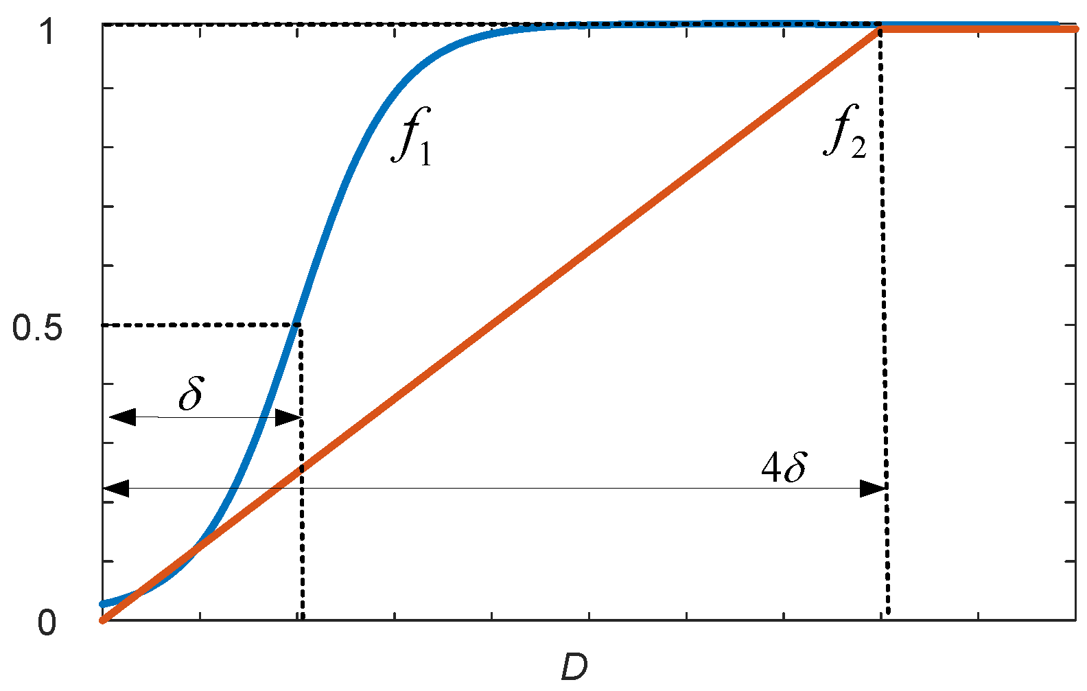
Figure 2 shows two example designs of
f:
, with a discontinuity point
, is a sigmoid-based CDF function, featuring a surge in the collision score (the derivative is bump-shaped) at the experience value around
. This function is suitable to important resources that are sensitive to the agent;
is a linear CDF with a shallow slope (the derivative is flat). This function can apply to trivial resources that are not very sensitive to the agent but still accumulate to contribute to the collision score. We use the offset parameter
to adjust the
tolerance level of the dissatisfying experience. With larger
, the agent will tolerate a longer unpleasant experience before announcing a collision.
Although the definition of the collision score can be customized according to different practices, the probabilistic definition of collision score introduced here is a general one: Different types of resources may have different value ranges, and Equation (
8) standardizes the resource ranges, mapping them to a value within
and enabling an efficient integration of different types of resources to the framework.
4.1.3. Definition 3 (Soft-Collision Function)
Now, according to the collision scores from Definition 2, we want to pick out the above-threshold agents and place them into the soft-collision set via the soft-collision function for the purpose of applying the sub-dimensional expansion.
Given a path
and corresponding resource experience
for the agent
j, the
soft-collision function of the agent
j is
where
T is the
threshold of collision. The definition of the
global soft-collision function is then defined as
Based on Definition 3, we can formally construct the soft-collision constraint on common resources and obtain the soft-collision constrained MAPP problem:
This problem setting is general and can be utilized to express the hard collision setting in Equation (
2) by setting
or changing the condition inside the indicator function of Equation (
6) to
with infinite cost.
4.2. SC-M* Description
SC-M* is a general solver to the MAPP problem in Equation (
11) by adjusting M* to the soft-collision constraints on common resources. The pseudocode for SC-M* is presented in Algorithm 2, where critical commands relative to the soft-collision constraint are underscored. In this algorithm, Lines 1–7 initialize each vertex
v in the vertex set
V with infinite cost from the source
(the cost of
itself is zero), set dissatisfying experience to zero and make collision set
empty. The initial open list contains
only (Line 8). In each iteration, SC-M* expands the first-ranked vertex
in the open list ordered by the total cost
(Lines 10 and 11). The algorithm terminates and returns the result if the expanded
is the destination
(Lines 12–14) or jumps to the next iteration if immediate collision occurs at
, i.e.,
(Lines 15–17). Line 18 constructs the
limit neighbors of
using Equation (
4). For each vertex
in
(Line 19), it adds
to the descendant set
of
(Line 20), updates the dissatisfying experience of
using Algorithm 1 (Line 21), and merges the immediate collision at
to its soft-collision set
(Line 22). On top of the new collision set of
, SC-M* backpropagates to update all the affected ancestor vertexes from
(see Equation (
3)) and adds them back to the open list for re-expanding (Line 23). After this collision set updating operation, if
is free from collision and has improved cost, the algorithm accepts the new cost by save the trace-back information and adding
to the open list for expansion (Lines 24–28). This process repeats until the open list is empty (Line 9) when no solution exists or the optimal solution is found (Lines 12–14).
| Algorithm 2. Soft-collision M*. |
| Input: : source joint vertex; : destination joint vertex; : joint configuration graph; A: list of resources |
| Output: Path finding results |
| 1: for all in V do |
| 2: .cost ← +∞ |
| 3: .exp ← all zero experience |
| 4: |
| 5: .traceBack |
| 6: end for |
| 7: .cost ← 0 |
| 8: open |
| 9: while open do |
| 10: open.sort() by v.cost+heuristic[v] //i.e., sort the open list from small to large |
| 11: open.pop() |
| 12: if then |
| 13: return back_track_path[] //optimal path found |
| 14: end if |
| 15: if then |
| 16: continue //skip the vertex in collisions |
| 17: end if |
| 18: conduct the construction of using Equation (4) |
| 19: for in do |
| 20: add to //note |
| 21: experience() //update experience using Algorithm 1 |
| 22: |
| 23: backpro_update( open) // 1) update all the affected soft-collision sets using Equation (3) |
| //2) add all affected vertexes back to open list (see reference [6] for details) |
| 24: if and .cost+.cost .cost then |
| 25: .cost ← .cost+.cost |
| 26: .traceBack |
| 27: open.add |
| 28: end if |
| 29: end for |
| 30: end while |
| 31: return no path exists |
SC-M* can make a transition from a decoupled individual A* () to a standard hard-collision constrained M* (), providing more flexibility to the performance of the algorithm with bounded soft-collision scores.
4.3. Completeness and Cost-Suboptimality
A MAPP algorithm is complete if it guarantees that it will either return a path, or determine that no path exists in finite time. An algorithm is optimal if it guarantees returning an optimal path if such a solution exists. SC-M* is complete and suboptimal conditioned on the soft-collision constraint (i.e., , for a given collision threshold T).
4.3.1. Completeness
Theorem 1. SC-M* is a complete algorithm.
Proof of Theorem 1. SC-M* inherits the sub-dimensional expansion from M* (i.e., it changes the
only when one of the soft-collision sets
changes). The algorithm applies A* in the updated search graph. Due to the merging operation applied to collision set
, as shown in Equation (
3),
for each vertex will change finite times (at most
m times, which is the number of agents). Because A* is complete, applying A* to a given
takes finite time to return a result. Therefore, SC-M* is complete. □
4.3.2. Cost-Suboptimality
Different from M*, which is optimal, SC-M* is suboptimal because Equations (
9) and (
10) only include the immediate conflicting agents to the soft-collision set; the agents that softly interfere with the conflicting agents in the upstream path are excluded. Those excluded agents also contribute to the announced collision (i.e., making the collision score above the threshold). Because of this, SC-M* cannot guarantee the
inclusion property, which is the basis to ensure the optimality in M* [
6]:
The optimal path for some subset of agents costs no more than the optimal joint path for the entire set of agents. Without the inclusion property, SC-M* may not guarantee cost optimality.
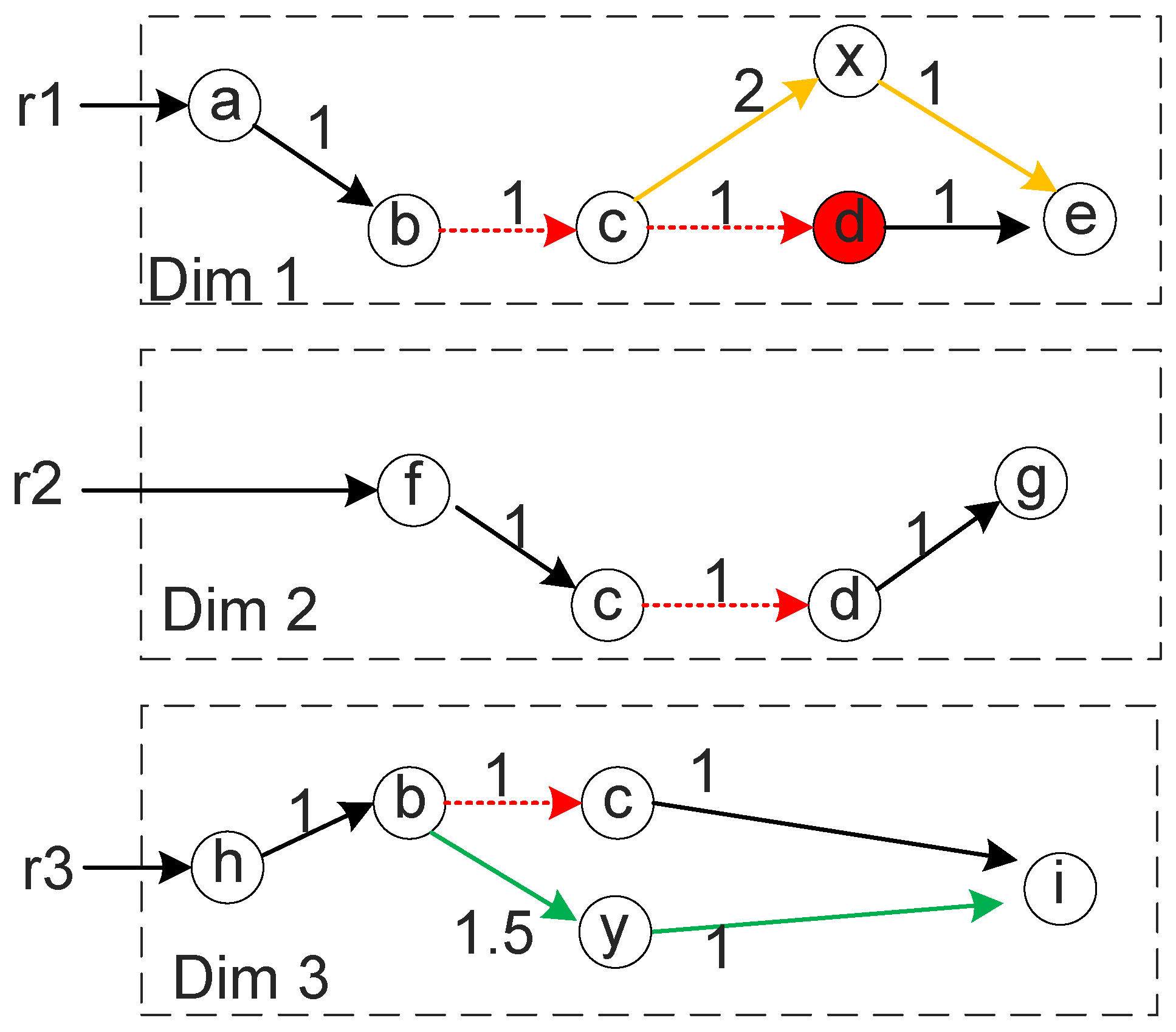
Figure 3 provides a counterexample of the inclusion property of SC-M* in the soft-collision MAPP context defined in this paper. Let
be the joint path constructed by combining the optimal path for a subset
of agents with the individually optimal paths for the agents in
. The inclusion property is defined as follows: If the configuration graph contains an optimal path
, then
,
. See
Lemma 6 in [
6].
In the soft-collision context, this inclusion property does not always hold. In
Figure 3, we have a three-agent MAPP problem (
) in the soft-collision context. Agents
,
, and
attempt to move from the vertexes
a,
f, and
h to the vertexes
e,
g, and
i, respectively. The individually optimal paths (shortest distance) are
with distance 4 for
,
with distance 3 for
, and
with distance 3 for
. The total cost of the joint individually optimal path is 10. However, assuming that the agents can only tolerate a dissatisfying experience with distance 1,
will announce a collision at vertex
d because of the interference on the edge
and
from agents
and
, respectively.
If we choose
, as can be seen in
Figure 3, the only solution would be that
takes a detour through the vertex
x to avoid the collision on the edge
, resulting in a cost of 5 for
, and the total
is 11 (3 for
, 5 for
and 3 for
). On the other hand, by searching through all three dimensions, a better solution would be that
detours through the vertex
y, and
is free from collision because the interference on the edge
disappears. The total cost of this joint path is 10.5, and we have
10.5, which is contradictory to the inclusion property.
The reason for this phenomenon is that, in the hard-collision context, only the immediate conflicting agent contributes to the collision of at vertex d. However, in the soft-collision context, both and contribute to the collision of at vertex d, and thus, the inclusion property does not apply. Without this inclusion property, which is the basis of the optimality of M*, the optimality of SC-M* cannot be guaranteed.
However, we notice that suboptimal methods have long been used successfully to solve many interesting MAPP problems [
15,
25,
26]. Given the fact that we show in the next section that SC-M* is superior to other alternative SC-based MAPP solvers (e.g., SC-A* and SC-CBS) in terms of scalability, run time, and path cost, we demonstrate that the proposed method, which is adjusted to MAPP in the soft-collision context, is a powerful tool in practice.
5. Experiments and Results
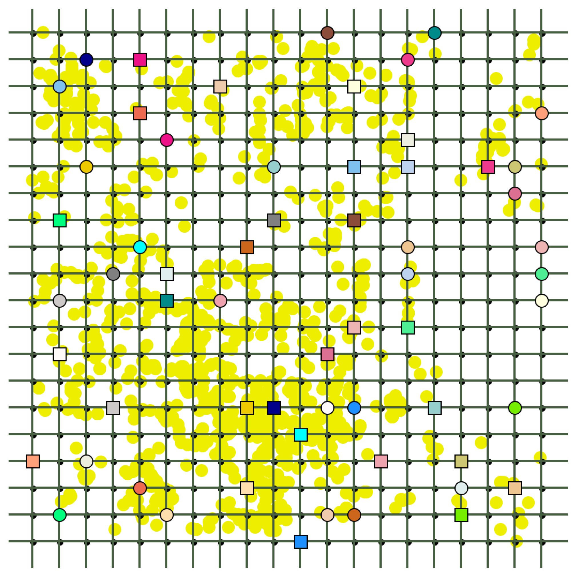
We evaluated SC-M* in simulation on a grid public mass transit network with an Intel Core i7-6700 CPU at 3.4 GHz with 16 GB RAM. As shown in
Figure 4, the grid transit environment has 20 × 20 stops. There are 20 bidirectional horizontal lines. Likewise, 20 bidirectional vertical lines are deployed in the environment. At each stop, agents can switch lines. The yellow areas are covered by some resources, such as the on-vehicle free Wi-Fi in our experiments. Agents traversing those areas can enjoy high-quality on-vehicle Wi-Fi connections. A fully covered edge has a Wi-Fi resource value of 100, and the Wi-Fi value of an edge is proportional to the length of coverage. Each agent wants to move from its source (square) to its destination (circle) with the lowest cost (i.e., a linear combination of distance cost and Wi-Fi cost) as well as bounded collision score. The second resource is the space on the edge, which is fixed at 5. The satisfying values are
and
for Wi-Fi and space resources, respectively.
We randomly generated a source–destination pair for each agent. Each trial was given a 1000-s run-time limitation to find a solution. For each configuration (including the number of agents, collision threshold T, and offset parameter ), we ran 20 random trials to calculate the average metrics (i.e., the success rate and run time). The success rate is the number of trials ending with a solution divided by the number of trials. The run time is the average over trials ending with a solution or a no-solution declaration. If all trials under a certain configuration exceeded 1000 s, we used “>1000” to represent the run time of the corresponding configuration. We used the standard A* as the coupled planner and policy generator in the SC-M* framework and compared our results to the baselines.
5.1. Planning for the One-Resource-One-Agent-Type
The first experiment considered Wi-Fi as the only resource requested by agents (i.e., ). Only one agent type exists, and all agents use sigmoid-based function as the collision CDF.
We first studied the influence of the collision threshold
T and the offset parameter
on performance.
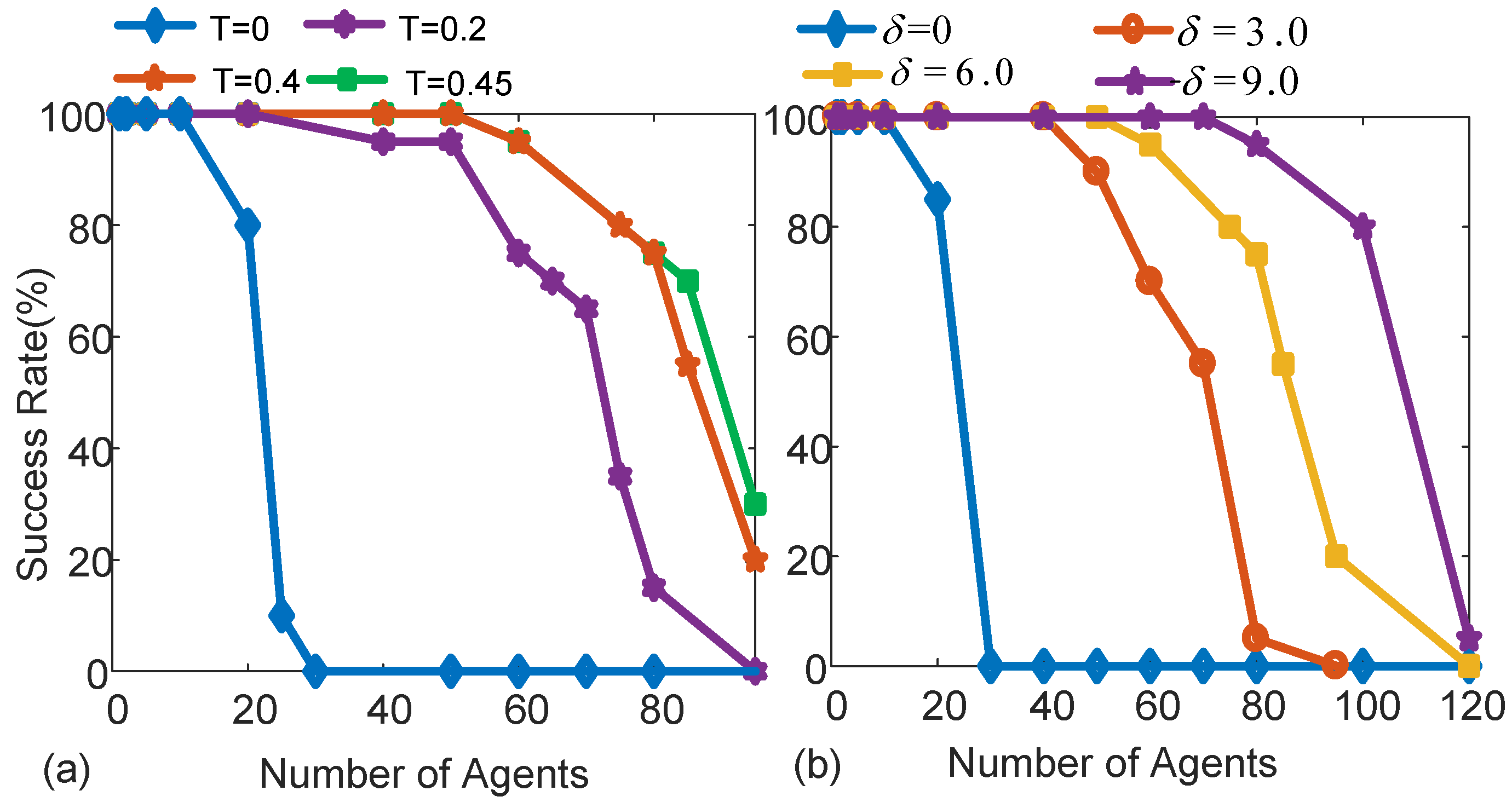
Figure 5a shows the success rate of the one-resource-one-type SC-M* with different thresholds
0 (equivalent to the basic M*), 0.2, 0.4, and 0.45, while the offset parameter is fixed to
.
Table 1 (left) shows the run time in seconds for the experiment. The results clearly show that larger thresholds bring improvement in performance with a higher success rate and lower run time for a large system size (
). The improvement in performance results from the property of SC-M* that larger thresholds render more relaxed constraints, and thus, agents are less likely to collide on resources.
Figure 5b shows the success rate of the SC-M* with different offset parameters
0, 3.0, 6.0, and
, with fixed
.
Table 1 (right) shows the run time for the experiment. The results illustrate that SC-M* is sensitive to
and can efficiently handle up to 100 agents with
. These results are reasonable because the sigmoid-based CDF is used in the experiments, featuring a surge in the collision probability at the experience value around the offset, and the offset parameter poses a cutoff value on the resource experience, with collision always announced once the resource experience is larger than the offset. The standard M* (
) can only scale to fewer than 30 agents. Taking advantage of this property, one can tune the parameters to trade off the scalability against the tightness of constraints.
5.2. Planning for the Two-Resource-Two-Agent-Type
We also evaluated SC-M* in more complex environments: two agent types requesting two resources. This experiment considered both Wi-Fi and space capacity (i.e.,
). Type I agents use
in
Figure 2 as the collision CDF for the Wi-Fi resource, and the linear CDF
for the space resource, implying that they treat Wi-Fi and space as important and trivial, respectively. On the other hand, Type II agents use
for space and
for Wi-Fi. Each agent has a 50% chance of being Type I. Both CDFs are adjusted using the same
at each trial, as illustrated in
Figure 2.
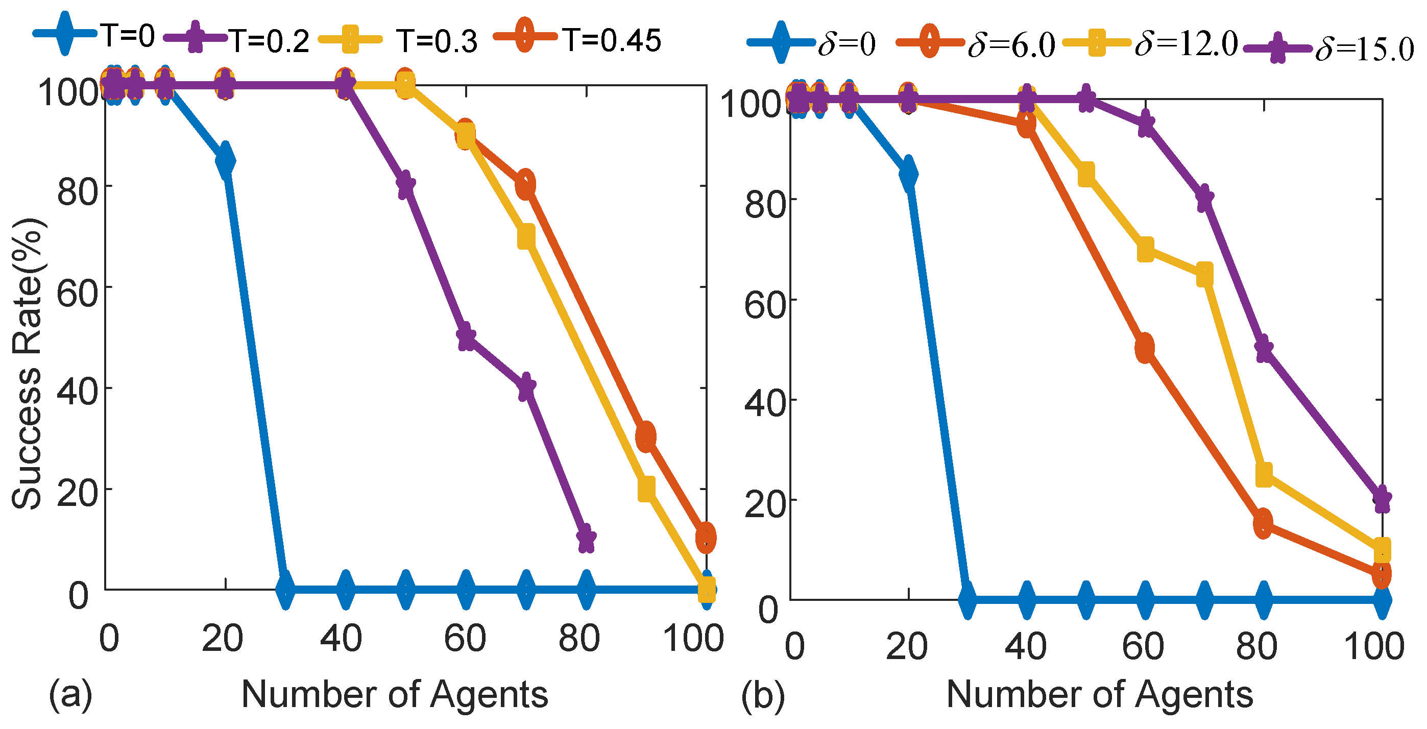
Figure 6a shows the success rate of the two-resource-two-type SC-M* with different thresholds
0 (equivalent to the basic M*), 0.2, 0.35, and 0.45, and with a fixed offset parameter
.
Table 2 (left) shows the run time for the experiments. As can be seen from the results, in general, SC-M* can handle the two-resource-two-type systems and plan for more than 80 agents. Because more resources contribute more factors to increasing the collision score, a relatively large offset (
) is needed to achieve comparable performance to the one-resource-one-type SC-M*.
Figure 6b and
Table 2 (right) present the impact of the offset parameter
on performance. Different from the first experiment, SC-M* with the above configurations is less sensitive to
, when compared to
Figure 5. The reason is that 50% of the agents are insensitive to one of the resources because of the linear CDF
, thus increasing
does not contribute to a significant reduction in collisions. This property implies that we can control the importance levels of resources efficiently through the design of collision CDFs. This experiment demonstrates that, with the proper parameter settings, SC-M* can feasibly handle a complex environment with multiple resources and multiple agent types.
5.3. Comparison of SC-M* to Baselines
We next compared the SC-M* to other SC-based MAPP algorithms, including SC-A* (optimal) and SC-CBS (suboptimal), in the one-resource-one-type environment.
5.3.1. Path Cost
Firstly, we compared the path cost of the three algorithms. We designed 60 planning tasks for environments with 4–6 agents (20 tasks for each), in which agents will encounter at least one collision along the individually optimal paths under the setting. We start with small agent numbers because SC-A* cannot handle a large number of agents.
Figure 7 shows the average difference of the three SC-based solvers relative to the individually optimal cost (i.e., the sum of the optimal cost of each agent when the agent is the only one in the system). In other words, the Y-axis represents the cost of collisions. We observe that SC-A* and SC-CBS have the lowest and highest additional cost, respectively. SC-M* solutions cost more than SC-A* but noticeably less than SC-CBS.
To be more detailed, in the experiments, we designed MAPP tasks for environments containing 4–6 agents with 20 tasks for each. All tasks were designed to encounter at least one collision along the individually optimal paths under the above-mentioned configuration. Thus, additional costs relative to the individually optimal path are expected for each of the three SC-based MAPP solvers.
Table 3 compares the results of SC-M* and SC-CBS to the optimal solutions obtained by SC-A*. The top half of the table shows the increase in cost relative to the cost for SC-A*; the costs for SC-A* for all scenarios vary within a small range so the results are in absolute numbers. The bottom half shows the ratio in run time with respect to SC-A*; the run time for SC-A* varies greatly across the experiments so we show the cost reduction as a percentage. In the table, we observe that the additional cost of SC-M* from the SC-A* is consistently lower than that of SC-CBS. We also observe that SC-M* is significantly faster than SC-A* and competitive relative to the run time of SC-CBS. The standard deviations show the fluctuations of the solutions for SC-M* and SC-CBS around the optimal solutions for SC-A*.
The reason for the results is that SC-A* is an optimal solver for this type of MAPP problem because it always explores cheaper paths in the entire multi-agent joint space before considering the paths that cost more [
7]. SC-M* is suboptimal because of the process discussed in
Section 4.3.2. Compared to SC-M*, SC-CBS suffers from more path cost due to the way it collects a collision: CBS collects collisions into a
conflict tree and arranges the collision into the form [agent
j, vertex
v, step
s], indicating that agent
j collides at vertex
v at step
s. In each iteration, CBS conducts decoupled planning to avoid agent
j reaching vertex
v at step
s. This might lose some information in the soft-collision context because there might exist another path that leads
j to vertex
v at step
s without announcing a collision, by avoiding one of the upstream vertexes involved in soft interference. In contrast, SC-M* can explore those paths excluded by SC-CBS because it searches the entire space of the immediate colliding agents.
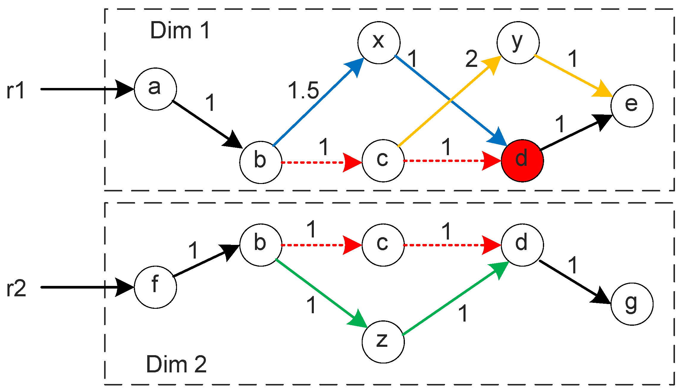
Figure 8 provides an example to visualize the difference in planning among the three SC-based MAPP solvers.
Figure 8 shows a two-agent MAPP problem in the soft-collision context. Agents
and
attempt to move from vertexes
a and
f to vertexes
e and
g, respectively. The individually optimal paths (shortest distance) for both agents are
with distance 4 for
and
with distance 4 for
, respectively. The total cost of the joint individually optimal path is 8.
and
softly collide on the edge
and
, where
can tolerate the dissatisfying experience with distance 2. However,
can only tolerate the dissatisfying experience with distance 1 and announces a collision at the vertex
d.
When using SC-CBS, we record the collision that occurred to as [, d, 3], indicating that agent will collide at vertex d at the third step. Then, SC-CSB will avoid any paths leading to d at Step 3 (including and ) and will end up with a longer detour through vertex y. The SC-CBS solution has a cost of 5 for and 9 in total.
When using SC-M*, the collision at d triggers the sub-dimensional expansion of the search graph in dimension 1, which includes both x and y. Thus, it can find a cheaper collision-free path through x and end up with a path with a dissatisfying experience of distance 1 and a cost of 4.5 for (8.5 in total). However, SC-M* does not expand dimension 2 because no collision has been announced by .
When using SC-A*, the joint search space of both dimension 1 and dimension 2 is expanded and searched. Instead of vertexes x and y, SC-A* will first investigate vertex z in dimension 2 according to some heuristics. This process leads to another cheaper path with distance 4 for (8 in total, which is the same as the individually optimal cost) and avoids all interference by moving through this path. As a result, SC-A* returns an optimal solution that satisfies the soft-collision constraint at the expense of search space.
The example in
Figure 8 illustrates the optimality of SC-A* and the advantage of SC-M* in path cost over SC-CBS. To be specific, SC-M* provides a better solution than SC-CBS by searching thoroughly through the expanded dimensions, whereas the way SC-CBS identifies collisions is inappropriate in the soft-collision context. To the best of our knowledge, no other methodology capable of dealing with the soft-collision path planning defined in Equation (
11) has been developed. It is expected that, in the future, more high-performance algorithms will be developed for solving the problem.
5.3.2. Run Time
Table 4 shows the average run time of the three SC-based MAPP solvers and we observe that both SC-M* and SC-CBS are significantly faster than SC-A* in terms of run time. This is reasonable because SC-A* always searches the global high-dimensional joint space, which is expensive. SC-CBS is faster than SC-M* because it always searches in one individual dimension at a time, whereas the SC-M* needs to occasionally deal with high-dimensional space when collisions occur.
5.3.3. Scalability
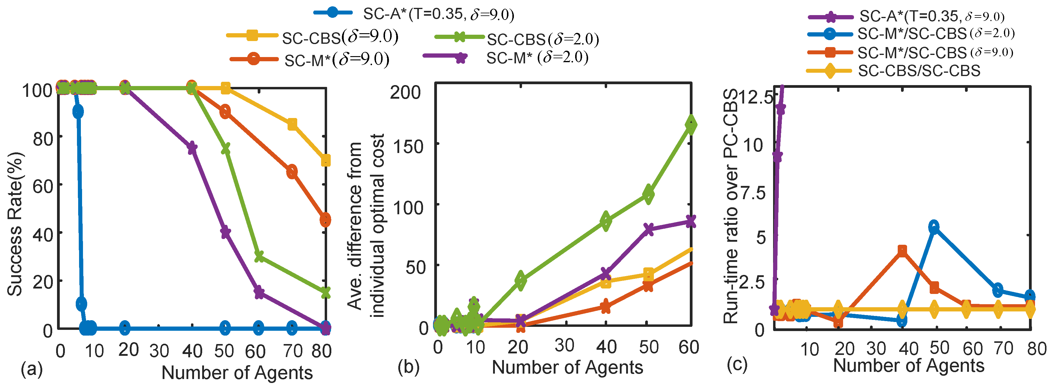
We compared the scalability of the three SC-based MAPP solvers in terms of planning for a large system size (
).
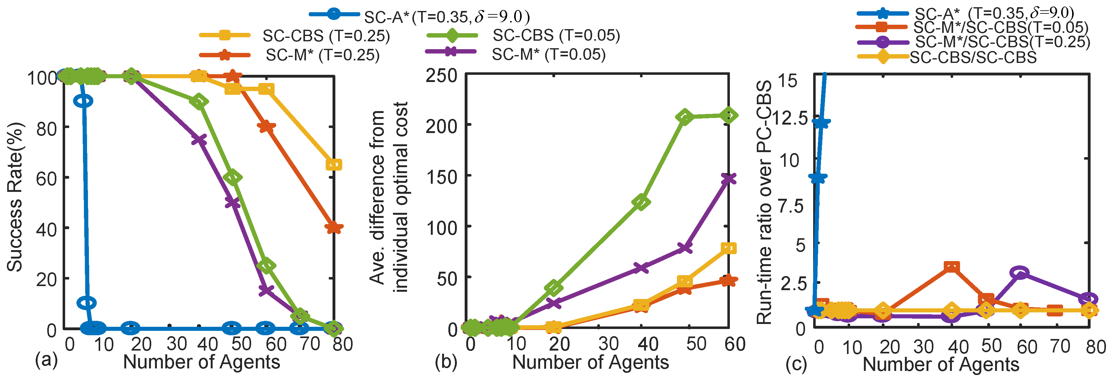
Figure 9 presents the success rate, average additional cost (i.e., how much more cost than the individually optimal path), and run-time ratio over SC-CBS under different thresholds
T, where the run-time ratio of SC-CBS is compared to itself and thus is constant. SC-A* has the slackest constraint (
) but poorest performance because of the prohibitively large search space. SC-CBS has the best success rate because of the property of the decoupled searching. However, this is at the expense of path cost. SC-M* performs decently in terms of both the success rate (significantly superior to SC-A*) and cost (noticeably lower than SC-CBS) as the number of agents increases.
The run time of the SC-M* is generally longer than that of SC-CBS. In another experiment, we observe that the run-time ratio of SC-M* over that of the SC-CBS starts to decrease after a peak. This is because we force all algorithms to terminate after 1000 s, and both curves will converge to value one when their success rates decline to zero. We conducted another scalability experiment with different offsets
(given
) and observe the same results in terms of scalability.
Figure 10 shows the experimental results.
Considering the scalability and path cost altogether, SC-M* demonstrates its overall advantages over alternative SC-based solvers.
6. Conclusions
This paper proposes SC-M*, a generalized version of M* with soft-collision constraints on common resources, which can scale to solving the multi-agent path planning problem in the soft-collision context. The SC-M* tracks the collision score of each agent and place agents, whose collision scores exceed some thresholds into a soft-collision set for sub-dimensional expansion. We show that the SC-M* has advanced flexibility and scalability for efficiently solving MAPP problems in the soft-collision context and can handle complex environments (e.g., with multiple types of agents requesting multiple types of resources). We compare the SC-M* to other SC-based MAPP solvers and show the advantages and trade-offs of the SC-M* against baselines in terms of path cost, success rate, and run time.
Future work will focus on leveraging advanced variants of M*, such as EPErM*, ODrM*, etc., to remove the basic A* component in our planner. We believe that better performance can be obtained this way because these variants improve the coupled planner and policy generator (two important components in the basic M*), which are directly related to the M* bottlenecks that limit the planning scalability. We are also interested in applying SC-M* to real-world applications for case studies. One promising research direction is to use the proposed algorithm to serve the passengers in public transits. It is expected that SC-M* will handle large-scale mobility demands in cities.
