Limited Search Space-Based Algorithm for Dual Resource Constrained Scheduling Problem with Multilevel Product Structure

Abstract

This study addresses the dual resource constrained flexible job shop scheduling problem (DRCFJSP) with a multilevel product structure. The DRCFJSP is a strong NP-hard problem, and an efficient algorithm is essential for DRCFJSP. In this study, we propose an algorithm for the DRCFJSP with a multilevel product structure to minimize the lateness, makespan, and deviation of the workload with preemptive priorities. To efficiently solve the problem within a limited time, the search space is limited based on the possible start and end time, and focus is placed on the intensification rather than diversification, which can help the algorithm spend more time to find an optimal solution in a reasonable solution space. The performance of the proposed algorithm is compared with those of a genetic algorithm and a hybrid genetic algorithm with variable neighborhood search. The numerical experiments demonstrate that the strategy limiting the search space is effective for large and complex problems.

1. Introduction

Several changes have occurred with the onset of the mass customization era following the traditional mass production era. Additionally, multipurpose machines and manufacturing processes have been adapted to flexible production systems producing a batch of small quantity [1]. In response to this trend, scheduling studies have focused on flexible manufacturing processes and have actively been conducted to solve the flexible job-shop scheduling problem (FJSP). In the FJSP research, various constraints, such as sequence dependent setup time [2,3,4], learning effect [5], and dual resource constraint [6,7,8], are considered depending on the manufacturing environment. This study deals with the dual resource constrained flexible job-shop scheduling problem (DRCFJSP) under the consideration of the worker’s skill level for machines and multilevel product structures (MLPS).

Research on the complexity of processes has been conducted, but there has been little research to reflect the complexity of product structures. The majority of the literature assumes a product structure composed of simple sequential operations for a job, which is very different from the bill of materials (BOM) structure that is widely used in manufacturing industries, especially for products requiring assembly processes. In several advanced planning and scheduling (APS) studies, the product complexity was reflected through the concept of MLPS. MLPS is a hierarchical tree that expresses the product structure and is essential for products requiring assembly processes. The top node of tree is a final product. Each child node of the tree represents a component or part of the product. With the MLPS, the operations for all the child nodes associated with the parent node must be performed, and then the operation for the parent node can be conducted. Chen et al. [9] developed a mixed integer programming model, which reflected the MLPS as a constraint; however, they only solved small-size problems with two orders. Dayou et al. [10] solved a multiobjective APS problem using a genetic algorithm (GA). To solve the structural problem of an MLPS, two chromosomes were constructed for the operation priority and machine assignment, respectively. The priority was randomly assigned through the operation priority chromosome, and the solution was constructed by assigning a feasible solution with the highest priority to a machine through the machine assignment chromosome. The performance and efficiency of the algorithm have been proven by experiments in 5 orders, 50 operations, and 20 machines. Chansombat et al. [11] focused on the determination of the operation sequence using the Bat algorithm. To solve the structural problems of the MLPS, the operation sequence was first determined and the solution feasibility was derived by correcting the misplacement of the items. In this study, unlike previous studies that separately determined the operation sequence and machine assignment, we propose a time-based integrated initial solution algorithm that allocates feasible operations and available resources (machine and worker), based on the priority rules that maintain solution feasibility and local search algorithms that narrow the search space using the earliest possible start time (EPST) and latest possible start time (LPST). In addition, previous studies determined the batch size based on the individual order quantity without considering the inventory level of the subparts and machine-dependent batch size, which is not suitable in environments where inventories exist and the batch size is required for the machine efficiency. Therefore, we combine the quantity of the subcomponents required for each order and generate the operations based on the inventory level and batch size.

The majority of the literature on scheduling considers only the machine as a constrained resource and ignores the constraints of worker availability required for the operations [12]. However, considering that the number of workers is limited in some manufacturing industries, scheduling without considering workers may be significantly different from the shop floor [6]. Studies have been conducted to solve the problem of co-considering the workers and machines as the dual resource constrained (DRC) scheduling problem. In particular, the dual resource constraints are investigated in the job shop and flexible job shop environments. The DRCFJSP has been studied using metaheuristic algorithms, such as GA [12,13], variable neighborhood search (VNS) algorithm [6,8], artificial bee colony algorithm [14], and memetic algorithm [15], because DRCFJSP adds another subproblem of worker assignment, which makes the problem complex, in addition to the machine assignment and operation sequence determination [16]. For example, EIMaraghy et al. [12] proposed a GA algorithm to solve the DRCFJSP in an environment with equal skill level of the workers. The allocation of the operations, machines, and workers was expressed as three chromosomes, and the superiority of the algorithm was proved by comparing it with the dispatching rules. Gong et al. [15] proposed a memetic algorithm for the DRCFJSP with multiobjective functions. The aim of the proposed algorithm was to minimize the makespan and workload of the machine and worker under the consideration of different worker skill levels. Lei et al. [8] proposed an efficient algorithm for solving the DRCFJSP by applying VNS. They demonstrated the performance of their algorithms in comparison with the GA. Wu et al. [6] proposed a hybrid algorithm combining the VNS and GA to solve the DRCFJSP considering worker’s learning ability. The VNS was applied to the populations, exhibiting a good performance. They demonstrated that the GA-VNS exhibits a better performance and lower relative percentage deviation than those of the GA and hybrid discrete particle swarm optimization.

The aforementioned metaheuristic algorithms are at risk of being isolated to the local optima due to the characteristics of the algorithm. Therefore, most metaheuristic algorithms prevent the solution from being isolated by introducing a wide variety of diversification, rather than concentrating on the intensification, to compensate for the weaknesses of the regional search algorithm. However, it is difficult to determine a feasible solution with many complicated constraints, and even intuitive improvements focused on intensification within a limited time are difficult due to the problem complexity. Therefore, exploring the solution space with a poor performance within the given computation time weakens the algorithm’s performance. Previous studies on the DRCFJSP were conducted by mitigating some constraints, such as worker skill, batch size, and complex product structure. In particular, the majority of the studies have developed algorithms for a simple product structure, and the metaheuristic algorithms demonstrated good performances. In this study, to deal with more complex problems with additional constraints, we propose a new local search algorithm that identifies a good search space and focuses on the intensification of a more likely space to compensate for the problem of diversification. In addition, the simple exchange of the operation sequence used in most scheduling algorithms in MLPS requires the process of solution repair for the feasibility. This results in heavy modification of the solution and increased computation time. Therefore, we use the priority rules to create a reliable initial solution for the time-based integrated initial solution algorithm, rather than the existing operation sequence expression, and derive an optimal schedule through the local search algorithm that limits the exploration space. To the best of our knowledge, our study is the first to propose an algorithm to solve the DRCFJSP that reflects the MLPS.

The remainder of this paper is organized as follows. Section 2 describes the environment and assumptions for the problem. Section 3 explains the proposed algorithm. In Section 4, we discuss the results based on the numerical experiments. Finally, some insights are discussed along with the conclusion and future research directions in Section 5.

2. Problem Description

The DRCFJSP can be applied in various industries including automobile industry, equipment industry [6] and electromechanical industry [17]. We consider DRCFJSP with an MLPS to deal with the scheduling problem of manufacturing systems with assembly lines. There is a set of orders, $O=\left\{O_1,O_2,...,O_n\right\}$; a set of final products $F=\left\{F_1,F_2,...,F_l\right\}$; a set of machines $M=\left\{M_1,M_2,...,M_m\right\}$; and a set of workers $W=\left\{W_1,W_2,...,W_k\right\}$. An order, $O_i$, denotes a production request for the final products, $F_a$, within the due date, $D{D}_i$. 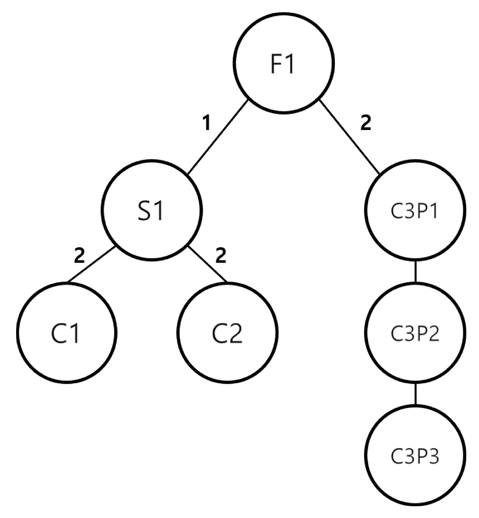MLPS is a hierarchical tree that expresses the BOM structure for a final product and subcomponents. To produce each upper element, various types of child components are required. In Figure 1, the numbers on the arcs connecting each node represent the number of child components required to produce the parent node. Figure 1 illustrates an example of the MLPS for a final product, F1, in Chen et al. [9]. F1 is produced by assembling one component S1 and two C1s, and C3 requires three successive processes, namely, P1, P2, and P3. When more than one process is required to produce a component, the process name is written along with the component name in the node. For example, in Figure 1, C3P1, C3P2, and C3P3 imply that the component C3 is processed in P1, P2, and P3, respectively.

Several constraints are considered for an environment of DRCFJSP with MLPS. First, MLPS must be considered to determine the schedule, i.e., a sequence of operations according to MLPS. For example, in Figure 1, the operations for C1 and C2 must be executed before S1. Second, each item and subitem can be processed only in the designated machines, and each worker can work on all machines. The processing time of an item depends on the assigned machine and the skill level of the worker. Third, each machine and worker cannot simultaneously perform more than two operations. The same type of item cannot be worked on machines at the same time. Finally, the production quantity is determined based on the lot size and the total demand. It must be greater than the demand and must be an integer multiple of the lot size.

In addition to the constraints, the following assumptions are made for the parameter values.

• The raw materials required for the operation of the items are sufficient.
• The operation setup time is small enough to be ignored.
• The lot-size of each operation is fixed.
• There is a difference in the skill level of each worker according to the machine; however, the improvement in the worker’s skill level because of the learning effect is small enough to ignore.

This study aims to minimize the lateness, makespan, and maximum deviation of the workload in the machines. Among these objective functions, lateness minimization has the highest priority, followed by makespan minimization and workload balance; the function with the highest priority is the most preferred. Equation (1) represents the objective function for lateness. Delays in delivery are one of the most important factors in the manufacturing environment, because frequent delivery violations and lateness cause financial damage by lowering the corporate trust and resulting in long-term declines in orders. Equation (2) minimizes the makespan, which is used in many scheduling studies as a measure of process productivity. Equation (3) represents the objective function for minimizing the deviation of workload between machines, and is used to prevent the imbalance of workload between machines. The notations used in this paper are summarized in

Table A1. Notations and symbols.

Notation	Explanation
i	order index, $i=1,2,3,...,n$
j	machine index, $j=1,2,3,...,m$
k	worker index, $k=1,2,3,...,w$
a	finished goods index, $a=1,2,3,...,a$
n	number of orders
m	number of machines
w	number of workers
M	a set of machine $M=\{M_1,M_2,...,M_m\}$
W	a set of worker $W=\{W_1,W_2,...,W_k\}$
F	a set of final item $F=\{F_1,F_2,...,F_a\}$
I${}_{\alpha }$	b-th stage c-th sub item of the final product a, where $\alpha$ is index set as $\alpha =(a,b,c)$
OL	operation list to produce
ML	a set of machines that can be operated
$M{L}^{{}^{\prime }}$	a set of idle machines
WL	allocable worker list
$I{S}_{\alpha }$	status of item $I_{\alpha }$, (if item $I_{\alpha }$ is ready to be processed: 0, otherwise: 1)
MS${}_j$	status of machine $M_j$, (if machine $M_j$ is idle: 0, otherwise: 1)
WS${}_k$	status of worker $W_k$, (if worker $W_k$ is idle: 0, otherwise: 1)
A${}_j$	list of operation that are selected from OL and can be produced on machine $M_j$
t	current time state
DD${}_i$	due date of order $O_i$
C${}_i$	completion time of order $O_i$
$p_{\alpha }$	processing time of item $I_{\alpha }$
p${}_{\beta }^{{}^{\prime }}$	processing time of operation $\beta$ considering Work skills
SL${}_{j,k}$	worker $W_k$ of worker’s skill level for machine $M_j$, ($S{L}_{j,k}\in [0.5,1]$)
WT${}_j$	total working time of machine $M_j$
CA	maximum working time per day
MC${}_j$	completion time of machine $M_j$
$c_{\alpha }$	completion time of item $I_{\alpha }$
$I{V}_{\alpha }$	inventory of item $I_{a,b,c}$
$S{I}_{\alpha ,x}$	inventory of the x-th sub item of $I_{\alpha }$
$N_{\alpha ,x}$	the amount of x-th sub item required to produce $I_{\alpha }$
LT	lot size
$s_{\beta }$	original start time of operation $\beta$
$s_{\beta }^{{}^{\prime }}$	modified start time of operation $\beta$

$$\left(G1\right)min\sum _{i=1}^n(D{D}_i-\left[\frac{C_i}{CA}\right])$$

(1)

$$\left(G2\right)min(max{C}_i)$$

(2)

$$\left(G3\right)min(maxW{T}_j-minW{T}_j)$$

(3)

3. Algorithm Based on Limited Search Space

3.1. Algorithm Process

Considering MLPS, DRCFJSP is difficult to solve because of many complicated constraints, especially complex product structure and dual resources. The development of an algorithm tailored for the problem is very important to find an optimal solution within a limited time. The rational logic behind the proposed algorithm is that spending more time within a good solution space is better than randomly searching the entire solution space. That is, we want to begin with a good initial solution and not spend much time on checking the feasibility of the solution generated from the local search algorithm. Therefore, we propose a time-based integrated initial solution algorithm in Section 3.2 and a local search algorithm in Section 3.3.

Figure 2a is a flow chart of the proposed algorithm, and Figure 2b,c shows GA and GA-VNS, respectively. The proposed algorithm has three unique features compared to GA and GA-VNS. First, the time-based integrated initial solution algorithm is used to find a good initial solution. In contrast to the method of randomly selecting an initial solution, the performance of the algorithm is improved and the computation time based on the three priority rules is reduced. Second, the limited search space algorithm is used to efficiently find candidate solutions. The problem with many constraints is a large infeasible space, and it is not easy to generate candidate solutions that do not change much compared to existing solutions while maintaining feasibility. Based on the concept of EPST and LPST for guaranteeing solution feasibility, we spend more time on generating candidate solutions within the limited search space. Third, we do not use a mutation operator to focus on intensification. A mutation operator can be introduced for diversification but it requires additional computation time.

3.2. Initial Solution

This section explains the time-based integrated initial solution algorithm. Using this algorithm, an initial solution is generated by assigning appropriate workers and operations to the available machines over time based on several priority rules. Before applying the priority rules, the operations are generated based on the inventory level and batch size as follows. First, the required production quantity is determined by comparing the order quantity and initial inventory level. Second, the operation quantity is determined as a multiple of the batch size at the time bucket with a positive production quantity. Third, the production quantity at the next time bucket is determined when the operation quantity is greater than the production quantity. The second and third steps are repeated as needed, and the same process is applied to the subitems according to the MLPS.

After generating a list of operations, three types of priority rules are applied for the initial assignment: operation rule, machine rule, and worker rule. First, in the case of the operation rule, a higher priority is randomly assigned to the orders that need to be fulfilled within a day, and a lower priority is assigned to the other orders. Second, according to the machine rule, an available machine with a smaller number of executable items has a higher priority. Figure 3 illustrates an example explaining the machine rule. There are three machines ($M_1$, $M_2$, and $M_3$) and five items ($I_{1,1,1}$, $I_{1,1,2}$, $I_{1,1,3}$, $I_{2,0,1}$, and $I_{3,0,1}$). All five items are executable on $M_1$, and $I_{1,1,1}$, $I_{1,1,2}$ and $I_{2,0,1}$ are executable on $M_2$. $M_3$ only produces item $I_{1,1,1}$. Therefore, the number of executable items of $M_1$, $M_2$, and $M_3$ are 5, 3, and 1, respectively. According to the machine rule, $M_3$ has the highest priority; thus, item $I_{1,1,1}$ is assigned to $M_3$, as depicted in Figure 3a. Then, $M_2$ becomes available with the smallest number of executable items; thus, an item is assigned to $M_2$. In this manner, all the items are assigned to the machines. In contrast, Figure 3b illustrates an example where an available machine with a larger number of executable items has a higher priority. In this case, most of the items are assigned to $M_1$, and $M_3$ becomes idle. This example demonstrates that the proposed machine rule is highly likely to derive a better solution in terms of the idle time, makespan, and workload of the machine. Finally, the worker rule identifies a worker with the highest skill for a machine among the available workers at the beginning of the production. To efficiently derive an initial solution, an available machine is selected based on the machine rule, and an appropriate worker with the highest priority is selected. Then, the item with the highest priority is assigned to the selected machine. Figure 4 and Figure A1 depict the flowchart and pseudocode for the time-based integrated initial solution algorithm.

3.3. Local Search

In this section, we propose a local search algorithm, named the limited search space (LSS) algorithm, to avoid the fluctuation of the solution performance. Candidate solutions are generated through the exchange of operations between different machines. First, after randomly selecting an operation, a list of exchangeable operations is generated by checking the machine compatibility and available time buckets. Machine compatibility can be easily checked by using the given data on the designated machines. The available time buckets in which an item can be processed is determined based on the EPST and LPST. EPST refers to the earliest time when all the sub items or raw materials are prepared so that the item is ready for the operation. LPST refers to the latest time that an item must be processed to avoid the delay of finished goods when compared to the previous solution. This process of checking the machine compatibility and available time buckets limit the search space; therefore, solution feasibility is always guaranteed even if there are many other constraints.

Next, the randomly selected operation is exchanged with an operation in the list of exchangeable operations to generate a candidate solution. The processing times of the exchanged operations can be changed depending on the worker skill level assigned to the machine. When the completion time of the operation is delayed when compared to the previous solution, it affects the schedules of the following operations. To maintain the efficiency of the algorithm, the same amount of delay is applied to all the operations that begin after the operation that causes the delay. Then, the candidate is generated by modifying the operation’s start time to be as early as possible based on the updated EPST and availability of worker and machine. Figure 5 depicts the pseudocode for the candidate generation.

Finally, the solution is updated based on the performance improvement in terms of the objective functions. Two approaches are employed for the solution update: limited space full search (LSFS) and limited space interactive search (LSIS). LSFS generates all possible candidate solutions using the list of exchangeable operations and determines the best solution. When a better solution is obtained, the solution is updated and moves to the first step of the algorithm. Otherwise, the algorithm is ended. In contrast, LSIS generates only one candidate solution and calculates the objective function value. When the objective function is improved, the solution is updated and immediately moves to the first step of the algorithm and searches a different part of the solution space. Otherwise, the next candidate solution is generated. After generating the candidate solutions one by one, the algorithm stops when the solution is not improved.

4. Numerical Experiments

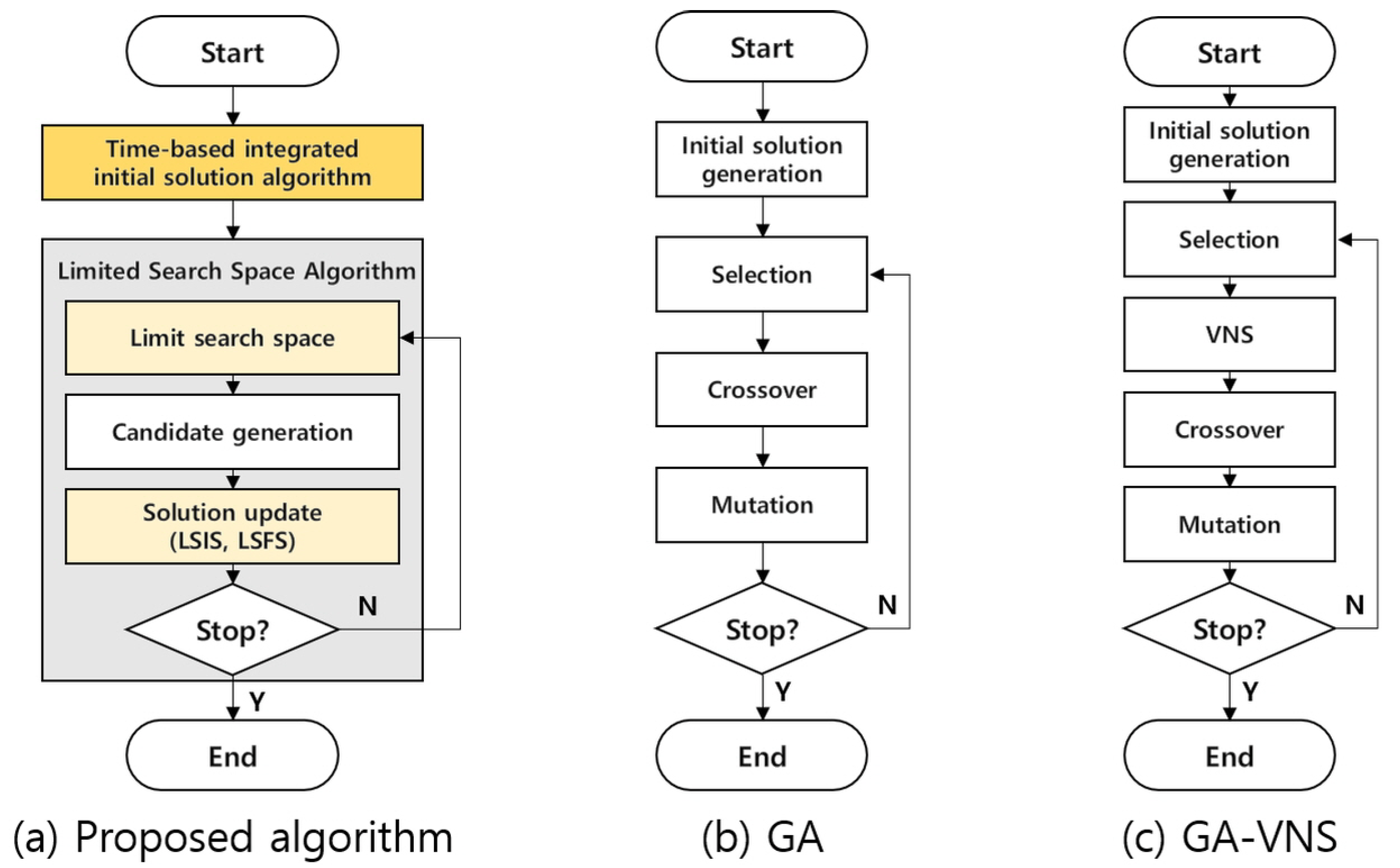
The superiority of the proposed algorithm is demonstrated through its comparison with the GA and GA-VNS. The overall algorithm structure of GA and GA-VNS is based on the previous study by Wu et al. [6]. As shown in Figure 2, GA proceeds through the procedures of initialization, selection, crossover, and mutation. The algorithm proposed by Wu et al. [6] was partially modified because it is not suitable for MLPS. In their problem, a final item requires a simple sequence of operations, and the order for a final item occurs only once. Therefore, it is easy to construct an operation sequence chromosome based on the final item. However, this is not appropriate when we consider MLPS and multiple orders for each item. The representation of the operation sequence chromosome based on the final item has a problem of uniqueness. Therefore, the decoding process is modified to consider the MLPS. The feasible suboperations required for the final product are selected based on the MLPS, and the sequence of suboperations is randomly selected if there are multiple feasible suboperations. The encoding and other parameter settings, such as crossover, mutation, elite, and tournament, are the same as those in the algorithm proposed by Wu et al. [6]. In particular, selection is performed through the elite tournament, and VNS is applied to the top 50% of the candidate s in the case of GA-VNS.

4.1. Evaluation of the Initial Solution Algorithm

To verify the effectiveness of the initial solution algorithm, we solve small scale problems. The experiment environment is described as follows.

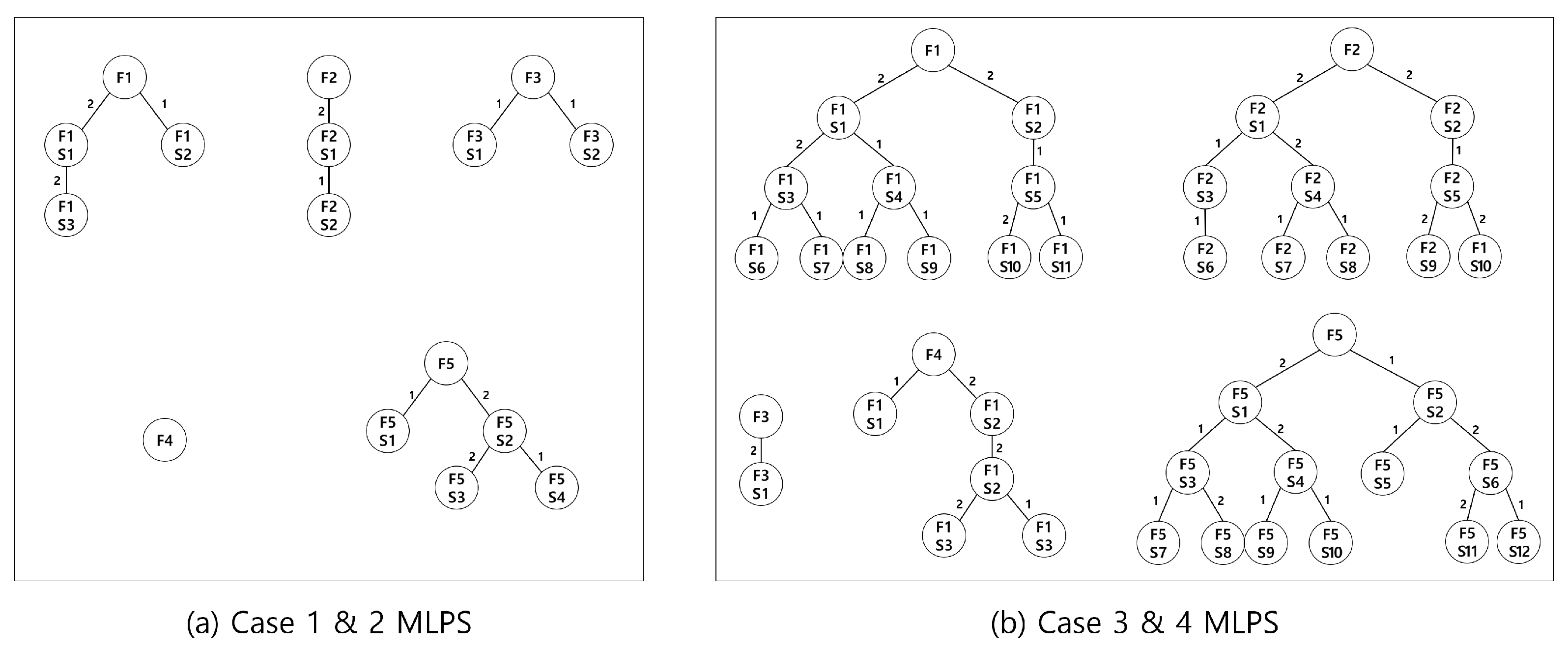
• The number of final items is five, and they have the BOM structure in Figure 6. In cases 1 and 2, a BOM can have up to two subparts for the upper part. In cases 3 and 4, the BOM structure is extended up to four levels.
• The time horizon is composed of seven time buckets, and the number of finished product s required in each time bucket can be up to 30.
• The processing time of each operation is randomly generated within a range from 1 to 15 time units.
• The number of machines is five. On an average, each machine can work on processing 30% items, and designated machines are randomly assigned.
• Capacity is either low or high. In the case of low capacity, the available time unit per day is 2000, and in the case of high capacity, 4500 units per day are available.
• The number of workers is three. The skill level of each worker is randomly generated within a range from 50 to 100%.
• Initial inventory level is zero.
• The lot size is 30.

Table 1. Result of Case 1 (low capacity: 2000; high capacity: 4500).

Algorithm	Low Capacity				High Capacity
	G1	G2	G3	Time (s)	G1	G2	G3	Time (s)
GA	17	15,789	5012	828	3	15,224	6616	864
GA-VNS	17	17,449	7780	2461	3	16,349	6037	2313
LSFS (w/o init)	20	20,325	6254	7200	4	19,573	5616	7200
LSIS (w/o init)	20	20,063	6254	2187	4	19,638	6363	6455
LSFS	7	10,794	3997	1122	2	13,841	5495	1911
LSIS	7	10,794	3997	1119	2	13,841	5495	955

and

Table 2. Result of Case 2 (low capacity: 2000; high capacity: 4500).

Algorithm	Low Capacity				High Capacity
	G1	G2	G3	Time (s)	G1	G2	G3	Time (s)
GA	21	14,952	5520	955	2	15,982	5068	899
GA-VNS	19	16,694	5672	2449	1	16,074	3497	2561
LSFS (w/o init)	21	16,574	5125	1115	6	18,106	5697	1749
LSIS (w/o init)	21	16,574	5125	1138	5	18,346	5697	1362
LSFS	8	9514	5055	3028	2	10,966	3838	1118
LSIS	8	9514	5055	1721	2	10,966	3838	1126

show numerical results with simple a BOM structure, as shown in Figure 6a. Order data is randomly generated within a range from 1 to 30, and other data remain the same. The performances of LSFS and LSIS are compared with those of GA, GA-VNS, and LSFS without initial solution algorithm, and LSIS without initial solution algorithm. In addition, the performance measures used are the objective function values (G1, G2, and G3) explained in Section 2 and computation time.

The results show that LSFS and LSIS with the initial solution algorithm are better than other algorithms. In particular, the performance gap between the algorithm with initial solution and without initial solution algorithm is quite large. As mentioned in the previous section, the main concept of the proposed algorithm is to begin with a relatively good starting point and improve the solution within the limited search space. It is also interesting that the computation time of LSIS and LSFS becomes shorter when the initial solution algorithm is applied. In other words, the performance of LSS-based algorithms is heavily dependent on the initial starting point, and the proposed initial solution algorithm plays a critically important role in achieving good performance. In addition, the performance of LSFS and LSIS is even worse than GA-based algorithms when the initial algorithm is not applied. Different from GA-based algorithms, the proposed algorithm does not use a mutation operator, and it can be worse than GA-based algorithms. The difference in the performances of LSFS and LSIS is not large. However, in terms of computation time, LSIS tends to be slightly superior to LSFS.

Next, we consider a more complex BOM structure shown in Figure 6b. We note that the proposed algorithm is terminated after 7200 seconds because it requires more computation time because of the complex BOM structure.

Table 3. Result of Case 3 (low capacity: 2000; high capacity: 4500).

Algorithm	Low Capacity				High Capacity
	G1	G2	G3	Time (s)	G1	G2	G3	Time (s)
GA	31	66,058	13,715	7119	30	66,222	14,396	6968
GA-VNS	31	65,290	15,119	18,637	28	14,907	19,598	18,776
LSFS (w/o init)	35	71,623	28,029	7200	35	71,623	28,029	7200
LSIS (w/o init)	35	71,623	28,179	7200	33	74,393	22,358	7200
LSFS	35	42,030	23,492	7200	25	42,170	17,537	7200
LSIS	35	42,030	23,492	7200	25	42,170	17,597	7200

and

Table 4. Result of Case 4 (low capacity: 2000; high capacity: 4500).

Algorithm	Low Capacity				High Capacity
	G1	G2	G3	Time (s)	G1	G2	G3	Time (s)
GA	31	70,146	13,346	9102	29	70,421	9432	9121
GA-VNS	29	67,457	19,511	25,124	30	70,150	21,991	24,444
LSFS (w/o init)	35	69,979	18,473	7200	35	76,612	19,561	7200
LSIS (w/o init)	35	70,219	18,818	7200	35	76,612	19,111	7200
LSFS	30	40,542	24,581	7200	29	44,108	27,505	7200
LSIS	30	40,542	24,641	7200	29	44,108	27,105	7200

summarize the results. In most cases, LSFS and LSIS perform better than the other algorithms, but GA performs well in case 3 with low capacity. Because of the nature of a small-size problem, in some cases, GA can be better than the strategy limiting the search space and requiring efforts in the local search, which is less efficient than randomly searching for a larger solution space. In both cases, the initial solution algorithm improves the performance of the algorithm.

4.2. Extended Experiments

The FJSP can be categorized into total FJSP and partial FJSP according to the machine compatibility. Cases 5 and 6 represent the partial FJSP, where each operation can be processed only on some machines [18], whereas case 7 represents the total FJSP, where each operation can be processed on all the machines. For extended experiments, we used a simple BOM structure, as in Figure 6a, and increased the problem size including the numbers of final items, machines, and workers.

In case 5, the data used for the experiments are same as those used in the previous section except for order data. In the cases of GA and GA-VNS, 10 iterations were performed with 20 populations due to the limitations in the computational time, unlike in previous studies that performed more than 20 iterations with over 100 populations. The other parameters are similar to those in the study conducted by Wu et al. [6] (ratio of crossover: 0.5; ratio of mutation: 0.5; ratio of elite: 0.2; ratio of VNS: 0.5).

Table 5. Result of Case 5 (low capacity: 2000; high capacity: 4500).

Algorithm	Low Capacity				High Capacity
	G1	G2	G3	Time (s)	G1	G2	G3	Time (s)
GA	4	7696.6	3279.2	2662.8	0	8215	3782.5	2953.5
GA-VNS	8	9200.8	3421.6	9475.7	0	12,121.7	3062.5	21,155.3
LSFS	6	8683.3	3541.6	9357.8	2	7899.2	2909.2	16,097.2
LSIS	7	8785	3503	4090	1	9135	4092.5	1532.9

presents the results of a numerical experiment in case 5. In this case, GA exhibits the best performance, as presented in Table 5.

Case 6 represents a larger problem in comparison with case 5, with 20 final items, 10 workers, and 10 machines. The environment contains more flexible processes, and the machines can process an average of 50% of the items. Due to the practical constraints on the computation time, the experiment was conducted by reducing the scale to 10 populations and 10 iterations. Additionally, the proposed algorithm was terminated after 7200 s.

Table 6. Result of Case 6 (low capacity: 2000; high capacity: 4500).

Algorithm	Low Capacity				High Capacity
	G1	G2	G3	Time (s)	G1	G2	G3	Time (s)
GA	70	16,235.8	6049.5	9068.7	6	18,694	5599.4	6978.4
GA-VNS	52	14,304.8	5231.6	19,612	6	16,531.9	5824.5	17,293
LSFS	9	9110	3258	7200	0	11,850.6	6863.6	7200
LSIS	9	9179	3258	7200	0	10,795.7	3826.5	7200

summarizes the results of the numerical experiment in case 6. As the problem becomes larger, the strategy limiting the search space becomes more efficient, which is different from the results of case 5. The LSS algorithm with LSFS and the LSS with LSIS are better than the GA-based algorithms in terms of all performance measures. The results demonstrate a good performance with a significant difference in terms of lateness in a shorter computation time. For example, at low capacities, the total delayed time units was 9 for the LSFS and LSIS with a computation time of 7200 s. However, the total delayed time units was 70 and 52 for the GA and GA-VNS, respectively, with a computation time of over 9000 s. At high capacities, the lateness is reduced in all algorithms; however, the LSS-based algorithms perform better than the GA-based algorithms.

Case 7 assumes the most flexible environment, in which all the machines can operate at all items. The number of final items, workers, and machines are 30, 10, and 10, respectively. Experiments are conducted under the same conditions as those of case 6.

Table 7. Result of Case 7 (low capacity: 4500, high capacity: 9000).

Algorithm	Low Capacity				High Capacity
	G1	G2	G3	Time (s)	G1	G2	G3	Time (s)
GA	82	30,953.5	5686.7	15,064	13	30,808.7	5096.6	14,714.3
GA-VNS	79	28,964.9	4801.3	38,014	12	28,862.3	5899.6	38,677.4
LSFS	31	19,396	7247.4	7200	0	27,981.7	7639.4	7200
LSIS	29	19,396	6849	7200	0	27,981.0	7223.0	7200

presents the results of a numerical experiment in case 7. The result of case 7 is similar to that of case 6. Both LSS-based algorithms outperform the GA-based algorithms in a shorter time. LSIS is more efficient than LSFS even in an environment with low capacity, which explores more search space in a shorter time as the problem becomes more complicated. Although the search space is limited, LSFS determines all the possible candidate solutions at each iteration. Therefore, it takes a longer time and does not perform well for more complex problems.

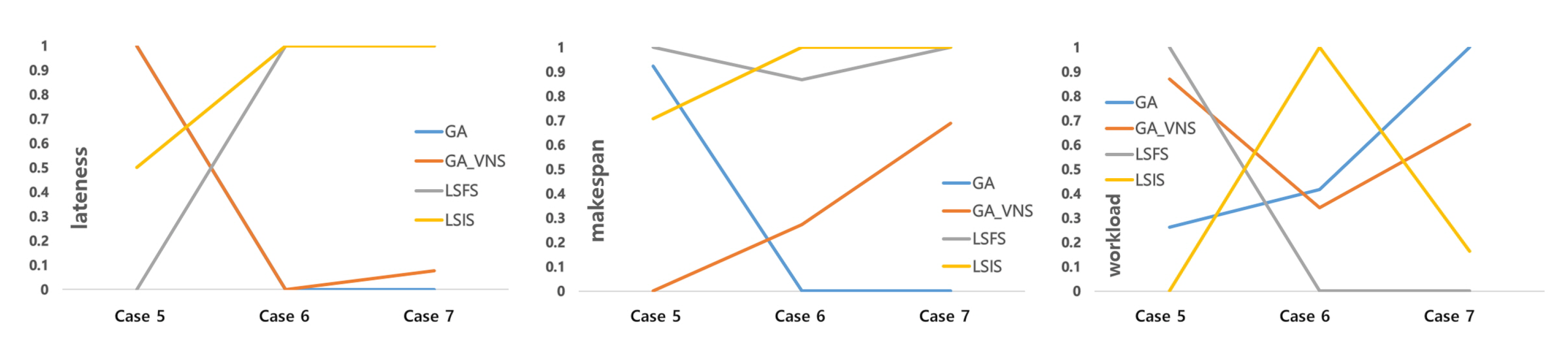
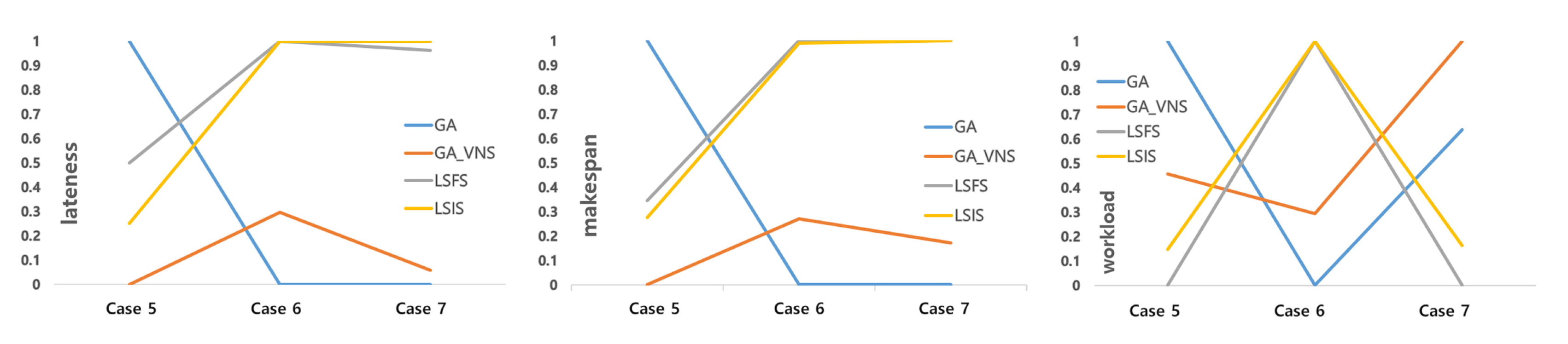
Figure 7 and Figure 8 illustrate the relative performance in comparison with the best solution, as the problem size increases in each capacity condition. The relative performance is calculated using Equation (4). The objective function values are normalized, and the best and worst solutions become 1 and 0, respectively. In terms of lateness, the objective function with the highest priority, the GA algorithm generates the best solution when the problem size is small, and the performance of LSIS is not the worst. However, as the problem size increases, LSIS generates the best solution or one that is very close to the best solution, and the performance of the GA algorithm becomes the worst. The performance of GA-VNS is similar to that of GA for cases 6 and 7. With respect to the makespan, the trend of the result is similar to that of the lateness, when the capacity is low. At high capacities, the LSS-based algorithms generate the best solutions or those that are very close to the best solution in all the cases. As for the third objective function, none of the algorithms outperform the others because this study considers a preemptive multiobjective approach, wherein the performance depends on the first and second objective functions.

$$Relativeperformance=\frac{Currentvalue-Minimumvalue}{Maximumvalue-Minimumvalue}$$

(4)

5. Conclusions

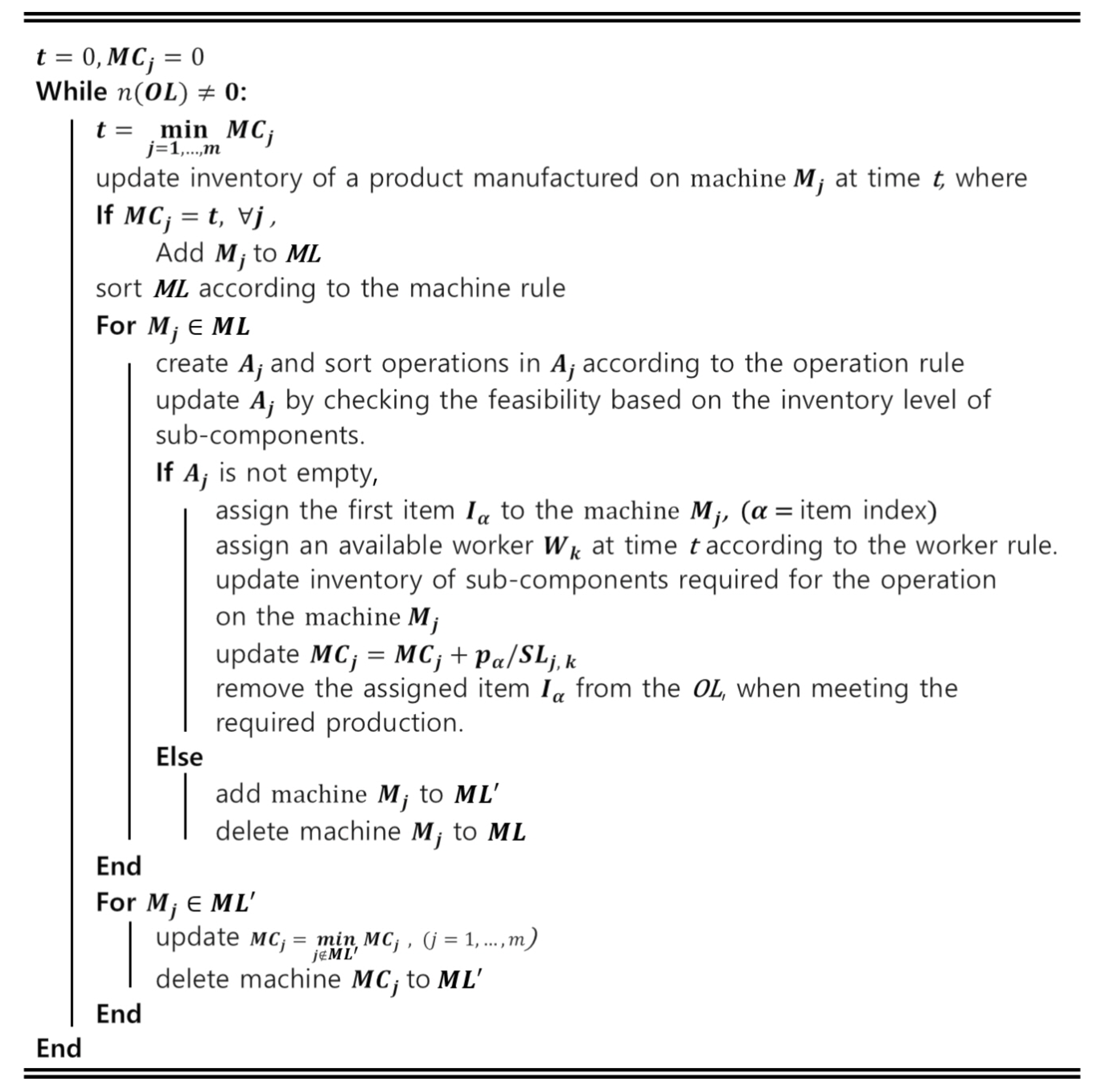
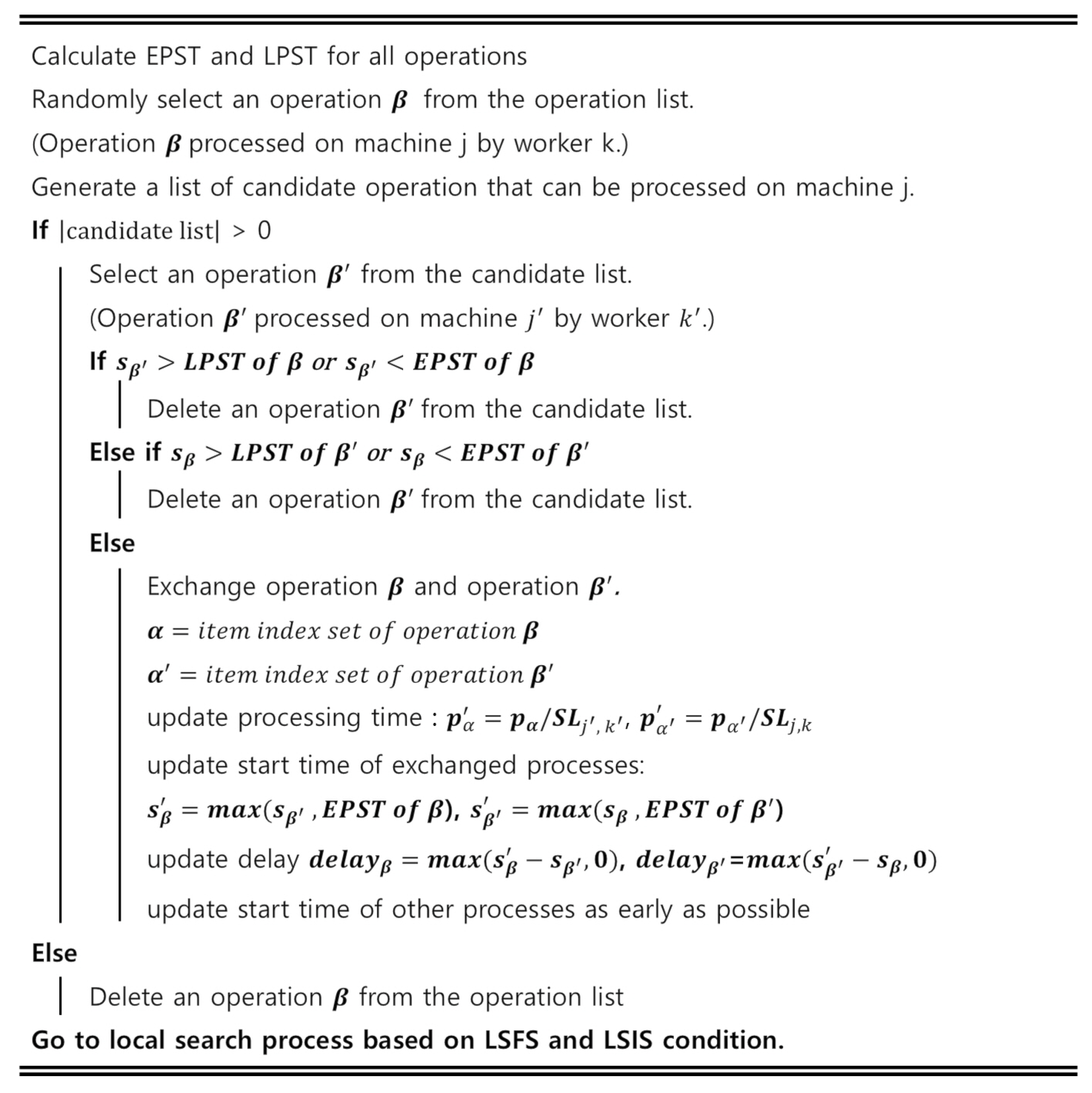
This study addressed the DRCFJSP under the consideration of worker’s skill and the MLPS. Due to the complexity of the problem, we proposed an efficient algorithm, limiting the search space to solve the complex DRCFJSP with three objective functions to minimize lateness, makespan, and machine workload distribution, which were improved sequentially. The algorithm was composed of a time-based integrated initial solution algorithm and LSS algorithm. The time-based integrated initial solution algorithm was tailored to the problem domain and modified the existing encoding method due to the unique characteristics of the MLPS. The LSS algorithm used the concept of EPST and LSPT to restrict the movement in the solution space, such that the previous solution was not considerably changed. In the limited search algorithm, the solution was updated using LSFS or LSIS.

Numerical experiments demonstrated that the proposed algorithm has an advantage for a complex problem when compared to the GA-based algorithms in terms of time and performance. In particular, when the problem size was small, the proposed algorithm was not always better than GA. In some cases, GA performed better than the proposed algorithm. However, for large-sized problems, we obtained better solutions in a shorter computation time by limiting the search space.

Further research is needed to develop extended models and algorithms considering additional constraints and uncertainties in the production system, such as the learning effect. The workers’ skill levels can be improved as the same work is repeated, and thus the efficiency can be changed. Various types of uncertainties must also be considered in future works. Because the actual manufacturing environment has various uncertainties, this research can be expanded to reflect the uncertain processing time, demand fluctuation, and machine failure. To overcome these issues, robust optimization and stochastic programming approaches can be applied.

The authors declare no conflicts of interest.