Indoor Localization Based on Wi-Fi Received Signal Strength Indicators: Feature Extraction, Mobile Fingerprinting, and Trajectory Learning

Abstract

This paper studies the indoor localization based on Wi-Fi received signal strength indicator (RSSI). In addition to position estimation, this study examines the expansion of applications using Wi-Fi RSSI data sets in three areas: (i) feature extraction, (ii) mobile fingerprinting, and (iii) mapless localization. First, the features of Wi-Fi RSSI observations are extracted with respect to different floor levels and designated landmarks. Second, the mobile fingerprinting method is proposed to allow a trainer to collect training data efficiently, which is faster and more efficient than the conventional static fingerprinting method. Third, in the case of the unknown-map situation, the trajectory learning method is suggested to learn map information using crowdsourced data. All of these parts are interconnected from the feature extraction and mobile fingerprinting to the map learning and the estimation. Based on the experimental results, we observed (i) clearly classified data points by the feature extraction method as regards the floors and landmarks, (ii) efficient mobile fingerprinting compared to conventional static fingerprinting, and (iii) improvement of the positioning accuracy owing to the trajectory learning.

Wi-Fi RSSI based indoor localization [1,2,3,4] is one of the standard approaches for indoor localization. It is able to utilize the RSSI measurements received from a large number of access points (APs) that are already built in construction. However, the Wi-Fi RSSI as a function of distance between a receiver (smartphone) and a transmitter (wireless AP) is nonlinear and varying due to interference of the indoor environments such as the other radio signals, walls, and obstacles. To address this problem, many machine learning based localization methods [5,6,7,8] have been developed, which learn a pattern of the RSSI measurements corresponding locations across the interested positioning area. In addition, due to its unbiased estimation capability, it is likely to be combined with other kinds of localization, such as pedestrian localization using inertial measurement unit (IMU) [9,10], visual localization [11,12], and magnetic sensor-based localization [13,14].

In particular, semisupervised learning algorithms have been recently suggested for efficient indoor localization, which reduce the human effort necessary for collecting training data [15,16,17,18,19,20]. For example, for indoor localization, a large amount of unlabeled data can be easily collected by recording only Wi-Fi RSSI measurements without requiring position labels, which can save resources for collection and calibration. By contrast, labeled training data have to be created manually. Adding a large amount of unlabeled data in the semisupervised learning framework can prevent the decrement in the estimation accuracy that occurs when using only a small amount of labeled data.

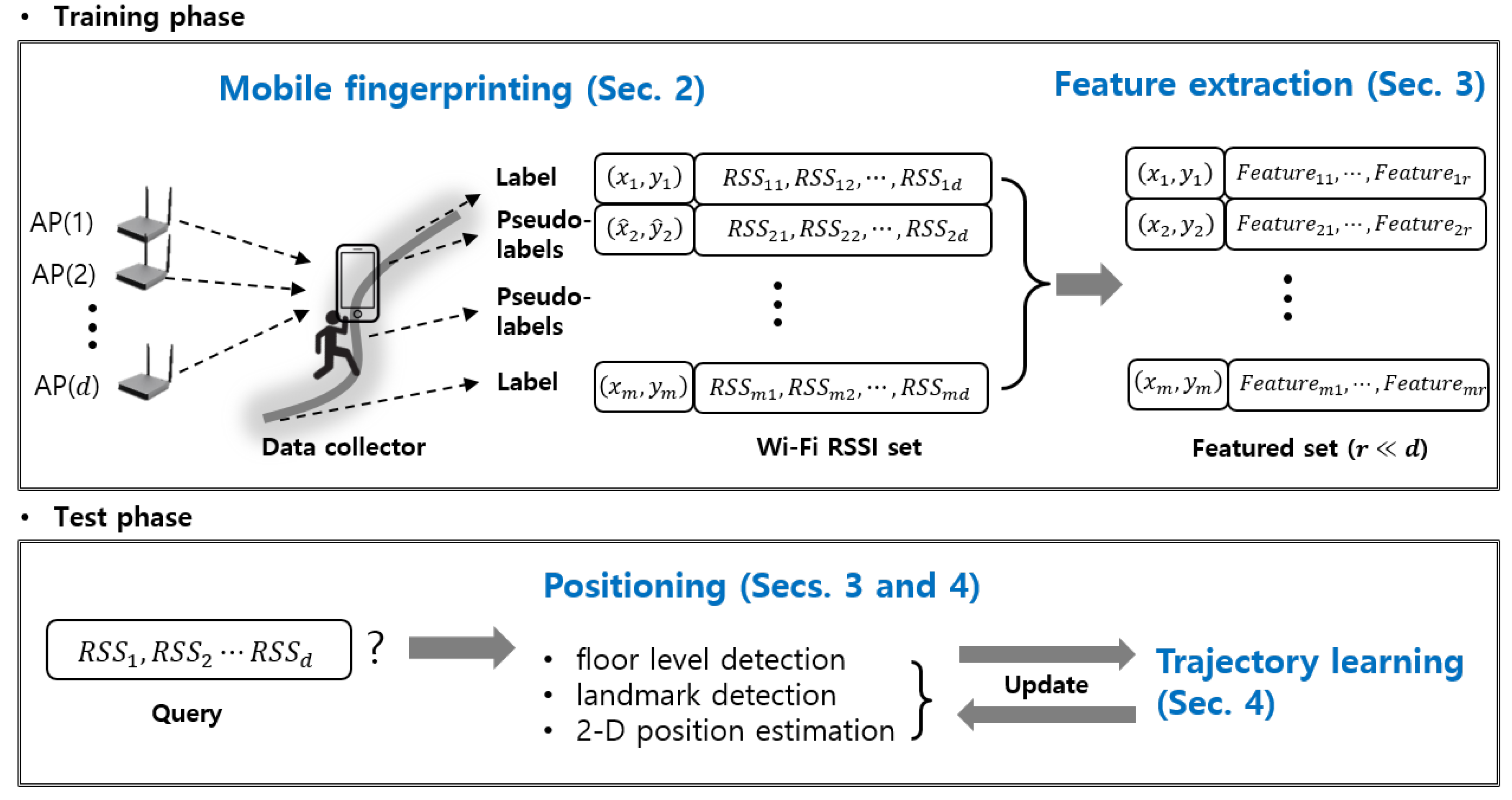
Given the advantage of semisupervised learning, this study describes (i) feature extraction, (ii) mobile fingerprinting, and (iii) mapless localization for efficient Wi-Fi RSSI-based localization. Figure 1 describes the interconnections between the research parts and the flow of our localization system.

First, the feature extraction considered in this paper aims to find a pattern from raw Wi-Fi RSSI and to reduce dimensionality. It allows not only recognizing different floor levels and different landmarks (e.g., toilet, room, and elevator), but also boosting calculation time. This study implements the multistory estimation including the classification of the floors and landmarks, by using the single Wi-Fi RSSI measurement set.

Second, most approaches to indoor localization have used the conventional static fingerprinting method in the training phase, where a trainer has to collect labeled training data stationarily at every position (or grid) while measuring and labeling Wi-Fi RSSI measurements. For more rapid and efficient collection, this study proposes the mobile fingerprinting method that allows a trainer to continue walking during the collection. Instead of the trainer’s necessity to label the positions corresponding the measurements, the proposed algorithm automatically pseudolabels (or estimates position of) the unlabeled data with a small amount of labeled data. For accurate pseudolabeling, we design a semisupervised regression by considering both the spatial and temporal relationship of the Wi-Fi RSSI sets.

Third, in indoor localization, it is common to apply a filtering method, such as a particle filter, to estimate the position or to boost accuracy [21,22,23]. However, this implies the assumption that a localization service provider can give the floor plan of the area of interest, which causes a large volume of data being transmitted to users. In this paper, the trajectory learning algorithm is integrated with the floor and landmark classification, mobile fingerprinting, and positioning for the expanded multistory building experiment.

Last, a position estimation algorithm is created by combining a particle filter and Gaussian process (GP) [24], to exploit the learned trajectories as a prior function and to use probabilistic GP likelihood by modeling the relationship between Wi-Fi RSSI and position.

We evaluate the proposed algorithms in a multifloor building through the experience of a few users. The experimental results show that (i) clearly classified data points with respect to different floors and landmarks by the feature extraction, (ii) efficient mobile fingerprinting compared to the conventional fingerprinting method, and (iii) improvement of positioning accuracy up to the average 1.2 m in comparison to standard approach thanks to the trajectory learning.

The paper is organized as follows. Section 1 surveys some studies relevant to indoor localizations. In Section 2, details about the mobile fingerprinting are presented. Section 3 examines characteristics of Wi-Fi RSSI and describes a semisupervised discriminant analysis for extracting features from raw Wi-Fi RSSI observations, with a description of floor classification and landmark detection. Section 4 introduces the mapless localization and Section 5 summarizes the experimental results. Finally, Section 6 presents the conclusion.

1. Related Studies

This section provides a survey of studies relevant to indoor localization. Different semisupervised learning techniques are reviewed for feature extraction in Section 1.1 and for mobile fingerprinting in Section 1.2. Mapless localization, in Section 1.3, describes trajectory learning and position estimation.

1.1. Semisupervised Feature Extraction

A Wi-Fi RSSI dataset consists of RSSI values corresponding to a user’s position, obtained from Wi-Fi access points (APs). The dimension of a raw Wi-Fi RSSI dataset is defined as the number of APs scanned in the entire area of interest in a building. Typically, the dimensionality is so high that it is impractical to perform real-time operations. Additionally, many of the elements in a raw RSSI database are usually empty because APs cannot cover a wide area. Therefore, reconstructing the data of a raw database is of paramount importance. Deep learning approaches [25,26,27,28] have been applied to the RSSI indoor localization. The high accuracy reported is due to its capability for feature extraction by the deep neural network structure, which learns complex pattern of the RSSI observations. The feature extraction in the standard deep learning except the autoencoder method [29] is computed among the hidden neural network layers, and then the hidden layers are connected to the latest localization layer. Thus, they cannot be used for our purpose to obtain the low-dimensional feature vector separately.

This paper combines two feature extraction methods: Fisher discriminant analysis (FDA) and principal component analysis (PCA). FDA is an a supervised dimensionality reduction method, and PCA is an unsupervised dimensionality reduction method. Supervised FDA tends to find embedded spaces overfitted to labeled samples. Therefore, it is effective to add unlabeled data, which can be collected easily and in large volumes. By using both labeled and unlabeled data, the combination of FDA and PCA can produce better accuracy compared to that achieved by solely using supervised FDA or unsupervised PCA. In this study, the role of semisupervised discriminant analysis is two-fold: dimension reduction and detection of floor level and landmarks.

1.2. Semisupervised Learning for Mobile Fingerprinting

In this section, the semisupervised learning methods for regression are presented, which are used to build the relationship between the Wi-Fi RSSI data sets and the locations. We then derive the contribution of the proposed mobile fingerprinting algorithm.

Utilization of the unlabeled data has been studied in the semisupervised learning to improve the efficiency and accuracy of the indoor localization. In those works, semisupervised deep learning methods [18,19,30] have been recently developed. The mobile fingerprinting requires the light computation and should be implemented as fast as the mobile device or the server deals with huge amount of the unlabeled data. Therefore, rather than the heavily computational deep learning methods, the support vector machine (SVM)-based [31] semisupervised learning algorithms are applied in this paper, which solves a convex optimization problem.

Semisupervised least square (SSL) [32] adds manifold regularization of unlabeled data into the standard Least Square SVR framework [33]. Because of its linearized setup, this algorithm is fast and useful for real-time application. Semisupervised colocalization (SSC) [34] builds an optimization framework consisting of a singular value decomposition, a manifold regularization, and a loss function. Because SSC estimates the locations of the APs as well as a target’s location, it requires the known locations of the AP, whereas SVR-based semisupervised algorithms do not. Moreover, the large number of tuning parameters and the heavy computation may be a burden. Both SSL and SSC apply the unlabeled data only for making a manifold regularization, through the graph Laplacian. Further progressed utilization of unlabeled data occurs in transductive support vector machine (TSVM) [35] and Laplacian Embedded Regression Least Squares (LapERLS) [36]. TSVM attempts to find the labels of unlabeled data and obtain the decision function. Because finding a solution requires searching all candidate-labels of the unlabeled data, TSVM is not feasible in most applications.

LapERLS introduces an intermediate variable as a substitute for the original labeled data. During the optimization process via Karush–Kuhn–Tucker (KKT) conditions, pseudolabels and a transformed kernel matrix are generated. Then, the pseudolabels and transformed kernel matrix are used as a substitution for the original labeled data and the original kernel matrix, respectively. This algorithm is useful for large-scale problems, due to the light computation necessary for obtaining the transformed kernel matrix, because the standard kernel matrix and Laplacian matrix are decoupled. However, LapERLS becomes inaccurate when only a small number of labeled training data points are used.

We adopt the idea of pseudolabeling from LapERLS because the pseudolabels can compensate for the lack of labeled data. To improve the accuracy of the pseudolabels, we propose adding a temporal relation to unlabeled training data that are collected as time-series. A study [37] employing a Hodrick–Prescott (H–P) filter that captures a smoothed-curve representation for a time series from training data is helpful for assigning time-series pseudolabels. Consequently, our pseudolabeling is able to consider both the spatial and temporal aspect of the training data sets. Note that this pseudolabeling technique based on this semisupervised regression is used for the mobile fingerprinting, not for estimating the user’s position.

1.3. Mapless Localization

Accommodating a mapless situation might be valuable for secure localization operations by keeping information private. The pedestrian localization based on IMU and camera sensors easily produces the integral error so the user should carefully hold the receiver such as smartphone stationary and should not rotate it. This limitation restricts its practical usage. This study eliminates the need to restrict the users’ behavior and the need to assume on the accurate signal propagation model.

Crowd-sourcing has been a useful tool for indoor localization. Because the crowdsourced data are collected from a huge number of different users conveying various mobile devices, it has potential to help solving challenging problems such as heterogeneous hardware [38] and security issues [39]. In this study, we apply crowdsourced data to learn the hidden trajectory and extract the floor plan, to compensate for the absence of true map information. The trajectory learning algorithm originates in demonstration learning [40]. For the purpose of this study, trajectory learning is combined with semisupervised feature extraction in Section 1.1.

Finally, as the position estimator, the particle filter is employed for two reasons: First, this filter can use the learned trajectories as a prior distribution. Second, in the particle filter framework, the likelihood function can be defined as the function referring to the relationship between the RSSI measurement sets and the positions. In this study, the likelihood is defined as the probabilistic model by the Gaussian process.

2. Mobile Fingerprinting Based on Semisupervised Learning

Wi-Fi fingerprint localization estimates a location by matching the currently received Wi-Fi RSSI measurements to those in a training database. For creating this database, the conventional fingerprinting method requires a trainer to manually labels all the Wi-Fi RSSI measurements at every point of the grid. Instead of the time-consuming conventional method, this section introduces a new mobile fingerprinting data collection algorithm that allows the trainer to continue walking without the stationary calibration. In the training phase for data collection, it is common sense that data collecters recognize which floor they are located on. Thus, the proposed mobile fingerprint method aims to obtain 2D position of the unlabeled data.

Suppose $y={[y_1,\dots ,y_d]}^{\mathrm{T}}\in R^d$ is the set of the Wi-Fi RSSI measurements received from d Wi-Fi APs. In 2-D space, the user’s location is defined as ($x_{\mathrm{X}}$, $x_{\mathrm{Y}}$). The l number of the labeled training data points are defined as the set ${\left\{(y_i,{[x_{\mathrm{X}i},x_{\mathrm{Y}i}]}^{\mathrm{T}})\right\}}_{i=1}^l$ with $y_i\in X\subseteq {\mathcal{R}}^d$. The u number of unlabeled data set ${\left\{y_i\right\}}_{i=l+1}^{l+u}$ comprises only the RSSI measurements.

It is desired to find the separate mappings $f_{\mathrm{X}}:X\to \mathcal{R}$ and $f_{\mathrm{Y}}:X\to \mathcal{R}$, which denote the relationships between Wi-Fi signal strength and location of the smartphone, using the labeled training data ${\left\{(y_i,x_{\mathrm{X}i})\right\}}_{i=1}^l$ and ${\left\{(y_i,x_{\mathrm{Y}i})\right\}}_{i=1}^l$, and the unlabeled data ${\left\{y_i\right\}}_{i=l+1}^{l+u}$. Because the models $f_{\mathrm{X}}$ and $f_{\mathrm{Y}}$ are learned independently, we omit the subscripts of $f_{\mathrm{X}}$, $f_{\mathrm{Y}}$, and of $x_{\mathrm{X}}$, $x_{\mathrm{Y}}$, for simplification.

In the SVM-based semisupervised learning framework, the optimization formulation is as follows,

$$\begin{array}{c}\hfill f^{*}=\arg \underset{f\in {\mathcal{H}}_k}{\min }c\sum _{i}V(y_i,x_i,f)+{\gamma }_A{\parallel f\parallel }_A^2+{\gamma }_I{\parallel f\parallel }_I^2,\end{array}$$

(1)

where V is a loss function; ${\parallel f\parallel }_A^2$ is the norm of the function in the Reproducing Kernel Hilbert Space ${\mathcal{H}}_k$; ${\parallel f\parallel }_I^2$ is the norm of the function in the low dimensional manifold; and c, ${\gamma }_A$, and ${\gamma }_I$ are the regularization weight parameters. To represent the manifold ${\parallel f\parallel }_I^2$, the method uses graph Laplacian, the so-called graph-based semisupervised learning, and it is also called a semisupervised support vector machine when we use an $ϵ$-insensitive loss function. Then, the solution is achieved by iterative quadratic programming. More details about the semisupervised algorithm can be found in [37].

2.1. Hodric–Prescott Filter

Let us describe a scenario of mobile fingerprinting where a trainer collects the training data during walking. The observations are naturally recorded in time-series. This section introduces capturing the temporal property from the mobile fingerprint data by exploiting the H–P filter [41]. By using the H–P filter, the optimization problem can be formulated as follows,

$$\begin{array}{c}\hfill \underset{f}{\min }\sum _{i=1}^K{\left(f\left(y_i\right)-x_i\right)}^2+{\gamma }_T\sum _{i=3}^K{\left(f\left(y_i\right)+f\left(y_{i-2}\right)-2f\left(y_{i-1}\right)\right)}^2\end{array}$$

(2)

where ${\left\{(y_i,x_i)\right\}}_{i=1}^K$ is the time-series labeled training data over discrete time horizon K. The second term renders the sequential functional values $f\left(y_i\right),f\left(y_{i-1}\right),f\left(y_{i-2}\right)$ on a line in the embedded space. The solution of Equation (2) in matrix form is

$$\begin{array}{c}\hfill f={\left(I+{\gamma }_{T}D{D}^{\mathrm{T}}\right)}^{-1}x,\end{array}$$

where $x={[x_1,\dots ,x_K]}^{\mathrm{T}}$ and

$$\begin{array}{c}\hfill D={\left[\begin{array}{ccccccc}0& 0& \cdots & \cdots & \cdots & \cdots & 0\\ 0& 0& 0& \cdots & \cdots & \cdots & 0\\ 1& -2& 1& 0& \cdots & \cdots & 0\\ 0& 1& -2& 1& 0& \cdots & 0\\ ⋮& ⋮& ⋮& ⋮& ⋮& ⋮& ⋮\\ 0& \cdots & \cdots & 0& 1& -2& 1\end{array}\right]}_{K\times K.}\end{array}$$

(3)

In the following section, this H–P filter-based optimization is combined with the semisupervised learning framework to assign the temporal aspect to the unlabeled data.

2.2. Semisupervised Pseudolabeling

Here, the semisupervised optimization to create accurate pseudolabels for the unlabeled data by considering both the temporal and spatial aspect is presented.

Given the labeled and unlabeled training data ${\left\{(y_i,x_i)\right\}}_{i=1}^K$ arranged in chronological order, the optimization for generating pseudolabels $\tilde{X}\in R^K$ is

$$\begin{array}{cc}\hfill & \underset{\tilde{X}\in R^n}{\min }\frac{c}{2}{E}^{\mathrm{T}}E+\frac{1}{2}{\mu }_1{\tilde{X}}^{\mathrm{T}}L\tilde{X}+\frac{1}{2}{\mu }_2{\tilde{X}}^{\mathrm{T}}D{D}^{\mathrm{T}}\tilde{X}\hfill \\ \hfill & \mathrm{subject}\mathrm{to}:\Lambda \tilde{X}-X=E,\hfill \end{array}$$

(4)

where $\Lambda$ is a diagonal matrix of trade-off parameters with ${\Lambda }_{ii}=1$ if $y_i$ is a labeled data point and ${\Lambda }_{ii}=0$ if $y_i$ is an unlabeled data point. ${\mu }_1$ and ${\mu }_2$ represent a trade-off relationship between spatial and temporal correlation, matrix D is defined in Equation (3), and $X\in R^K$ is given by

$$\begin{array}{c}\hfill X=\left\{\begin{array}{c}\begin{array}{cc}{x}_i& \mathrm{if}{y}_i\mathrm{labeled}\end{array}\\ \begin{array}{cc}0& \mathrm{else}\mathrm{if}{y}_i\mathrm{unlabeled}\end{array}\end{array}\right.,\end{array}$$

and graph Laplacian L is defined as $L=B^{-1/2}(B-C)B^{-1/2}$, with the adjacency matrix C and the diagonal matrix B given by $B_{ii}={\sum }_{j=1}^K{C}_{ij}$. In general, the edge weights $C_{ij}$ are defined as a Gaussian function of Euclidean distance, given by

$$C_{ij}=\exp \left(-\parallel x_i-x_j{\parallel }^2/{\sigma }_w^2\right),$$

where ${\sigma }_w^2$ is the kernel width parameter.

With the introduction of a multiplier ${\alpha }_P$, the Lagrangian of Equation (4) is given by

$$\begin{array}{c}\hfill L=\frac{c}{2}{E}^{\mathrm{T}}E+\frac{1}{2}{\mu }_1{\tilde{X}}^{\mathrm{T}}L\tilde{X}+\frac{1}{2}{\mu }_2{\tilde{X}}^{\mathrm{T}}D{D}^{\mathrm{T}}\tilde{X}+{\alpha }_P\left(\Lambda \tilde{X}-X-E\right)\end{array}$$

(5)

The derivatives of Equation (5) with respect to the variables $\tilde{X}$, ${\alpha }_P$, and e set to zero are

$$\begin{array}{ccc}\hfill \frac{\partial L}{\partial \tilde{X}}& =& {\mu }_{1}L\tilde{X}+{\mu }_{2}D{D}^{\mathrm{T}}\tilde{X}+\Lambda {\alpha }_P=0\hfill \end{array}$$

(6)

$$\begin{array}{ccc}\hfill \frac{\partial L}{\partial e}& =& cE-{\alpha }_P=0\hfill \end{array}$$

(7)

$$\begin{array}{ccc}\hfill \frac{\partial L}{\partial {\alpha }_P}& =& \Lambda \tilde{X}-X-E=0\hfill \end{array}$$

(8)

Substituting Equation (7) into Equation (8) gives

$$\begin{array}{c}\hfill \Lambda \tilde{X}-\frac{1}{c}{\alpha }_P=X.\end{array}$$

(9)

Then, the linear algebraic equations satisfying the KKT conditions are defined as follows,

$$\begin{array}{c}\hfill \Phi A=F,\end{array}$$

(10)

where

$$\begin{array}{c}\hfill \Phi =\left[\begin{array}{cc}{\mu }_{1}L+{\mu }_{2}D{D}^{\mathrm{T}}& \Lambda \\ \Lambda & -\frac{1}{c}\end{array}\right]\end{array}$$

(11)

and,

$$\begin{array}{c}\hfill A=\left[\begin{array}{c}\tilde{X}\\ {\alpha }_P\end{array}\right],F=\left[\begin{array}{c}0\\ X\end{array}\right]\end{array}$$

(12)

Therefore, the optimal pseudolabels are obtained by inverse calculation of the matrix $\mathrm{\Phi }$. The advantages of this optimization compared to traditional semisupervised learning are as follows.

• A closed-form solution can be obtained from the linear algebraic Equation (10), which is faster than for other semisupervised algorithms and requires an iterative quadratic programming (QP) solver.
• The solution for $\tilde{X}$ also inherits the sparsity characteristics of a support vector machine [42]. This is beneficial when we manage training data storage by saving reliable training data only, that is, large values of ${\alpha }_P$ i.e., the support vectors.
• In addition to spatial representation, a time-series representation is considered, where the relevant term, ${\mu }_{2}D{D}^{\mathrm{T}}$, is inserted independently into the optimization problem. Without a substantial increase in computational time, it improves the accuracy of the pseudolabels. Its performance is analyzed in the next section.

In a summary, we address the role of the mobile fingerprinting and the connection to the next sections. The mobile fingerprinting is a method for database construction. Especially, it is useful when amount of the labeled data is not enough by its capability of accurately labelling the positions of the unlabeled data. As shown in Figure 1, the calibrated data from the mobile fingerprinting are used for the following feature extraction in Section 3 and the localization in Section 4.

3. Feature Extraction and Application to Floor Classification and Landmark Detection

Section 3.1 overviews the characteristics of Wi-Fi RSSIs and the need for feature extraction. Section 3.2 describes a semisupervised discriminant algorithm for the floor classification and landmark detection.

3.1. Wi-Fi RSSI Characteristics

This section examines characteristics of Wi-Fi RSSIs and discovers the necessity of the feature extraction for Wi-Fi RSSI-based indoor localization.

3.1.1. Nonlinearity and Uncertainty

According to a propagation model of Wi-Fi RSSIs [43,44,45], the RSSI value decreases exponentially when the distance between a transmitter and a receiver increases linearly. In reality, however, the interruption of the multipath generates uncertain Wi-Fi RSSIs because of the existence of a number of walls and the interference from other radio signals.

For validation, we record Wi-Fi RSSI values on an office floor shown in Figure 2a. Figure 2b shows the RSSI values according to the distance from Wi-Fi AP2; one graph shows the RSSI curve when a user moves along the corridor and the other is when the path is interrupted by walls. Because this study does not assume the that a map is available, it is impossible to predict the change in RSSI patterns with respect to the distance.

3.1.2. Sparsity

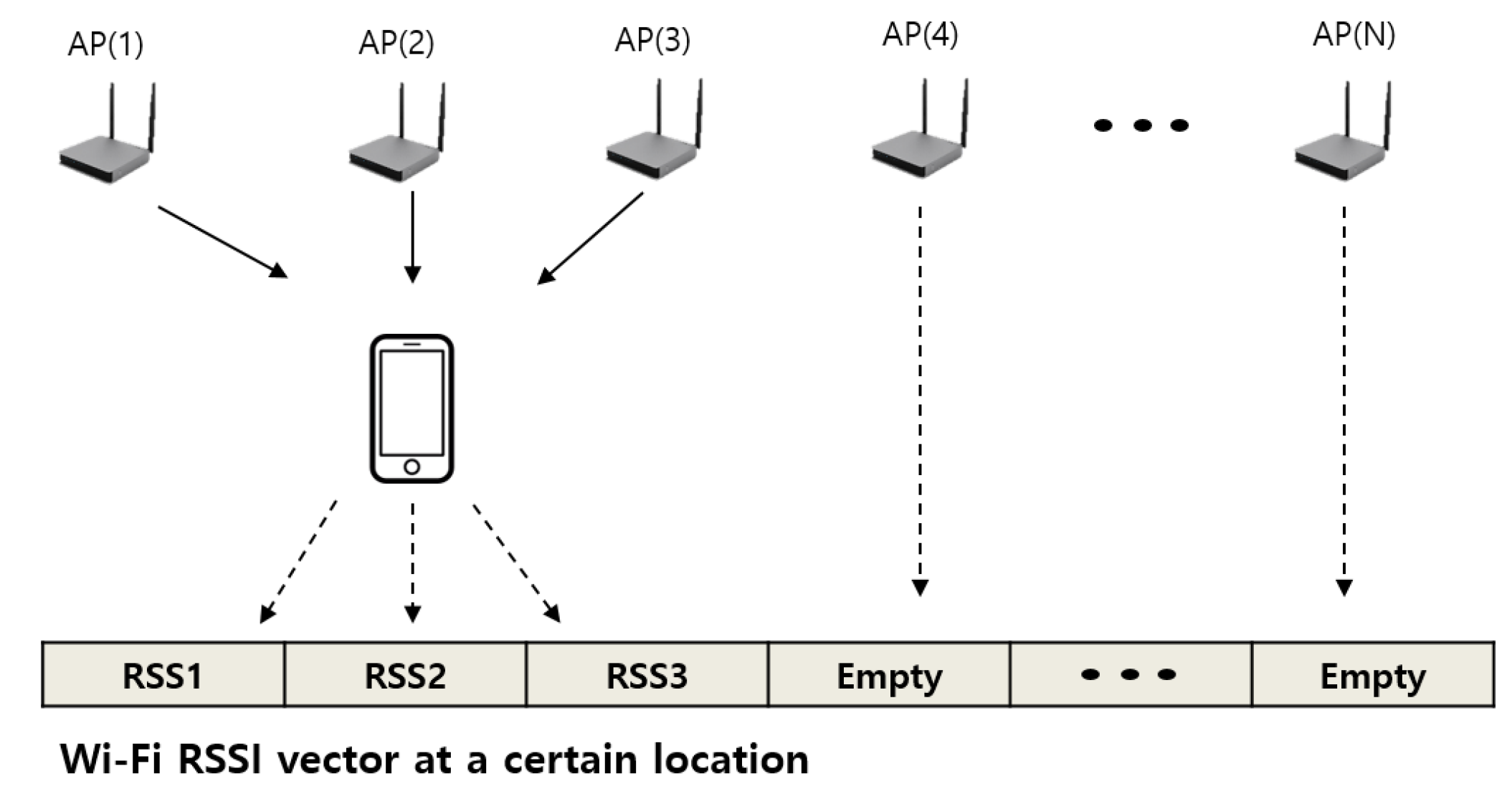
The other important characteristic is the sparsity of the raw Wi-Fi RSSI measurements. In a typical building, many Wi-Fi APs are installed, such as commercial APs, private internet-connected devices, and WLAN printers. For example, 193 APs were scanned in our experimental floors, and 531 APs are used in the the UJIIndoorLoc open dataset [46].

Not all the APs can be scanned at one point position because a single AP does not cover the entire positioning area. Thus, the RSSIs of APs located far from a user are recorded empty, as illustrated in Figure 3. The typical method to deal with the empty elements is to replace them by the possibly minimum RSSI value, e.g., −100 dBm. However, the sparsity still exists because the minimum RSSI values replace most of the elements, which may deteriorate localization performance. Therefore, we need to extract a feature. Further, substantially reduced dimensionality is helpful to reduce computational load.

3.2. Semisupervised Discriminant Analysis

Both principal component analysis (PCA) and Fisher discriminant analysis (FDA) have been widely used for feature extraction. These methods play the role of reducing dimensionality by highlighting meaningful elements from the original data vector. FDA is a supervised learning as it uses only labeled data, and PCA is an unsupervised learning because it uses only unlabeled data. The combination of FDA and PCA is categorized into the semisupervised learning.

3.2.1. Generalized Eigenvalue Problem

Remember that $y={[y_1,\dots ,y_d]}^{\mathrm{T}}\in R^d$ is the set of the raw Wi-Fi RSSIs. The feature set is given $z\in R^r$$(1\le r\le d)$, which is the resultant low-dimensional set by a feature extraction implementation. Let $T\in R^{d\times r}$ be a transformation matrix; then, it has the following relationship,

$$\begin{array}{c}\hfill z=T^{\mathrm{T}}y,\end{array}$$

(13)

where ${·}^{\mathrm{T}}$ represents the transpose operation. Both FDA and PCA solve the following optimization problem,

$$\begin{array}{c}\hfill T^{\mathrm{opt}}={\mathrm{argmax}}_T\left[\mathrm{tr}\left(T^{\mathrm{T}}BT{\left(T^{\mathrm{T}}CT\right)}^{-1}\right)\right],\end{array}$$

(14)

where B is a quantity we want to increase, C is a quantity to be hopefully decreased, and $\mathrm{tr}(·)$ represents the trace of a matrix.

Further, suppose that ${\left\{{\lambda }_i\right\}}_{i=1}^d$ is the set of generalized eigenvalues and ${\left\{{\phi }_i\right\}}_{i=1}^d$ is the set of the corresponding generalized eigenvectors. Then, the generalized eigenvalue problem can be defined as

$$\begin{array}{c}\hfill B\phi =\lambda C\phi .\end{array}$$

(15)

The generalized eigenvectors are orthogonal to matrix C:

$$\begin{array}{c}\hfill {\phi }_i^{\mathrm{T}}C{\phi }_j=0,\end{array}$$

(16)

for $i\ne j$, and the eigenvectors are normalized:

$$\begin{array}{c}\hfill {\phi }_i^{\mathrm{T}}C{\phi }_i=1\mathrm{for}i=1,2,\cdots ,d.\end{array}$$

(17)

Additionally, assume that the eigenvalues are organized in descending order:

$$\begin{array}{c}\hfill {\lambda }_1\ge {\lambda }_2\ge \cdots \ge {\lambda }_d.\end{array}$$

(18)

Finally, the transformation matrix can be summarized as

$$\begin{array}{c}\hfill T^{\mathrm{opt}}=\left(\sqrt{{\lambda }_1}{\phi }_1|\cdots |\sqrt{{\lambda }_r}{\phi }_r|\cdots |\sqrt{{\lambda }_d}{\phi }_d\right).\end{array}$$

(19)

From Equation (19), it can be seen that the influence of the transformation becomes deemphasized as the dimension order increases, because the eigenvalues and eigenvectors are decreasing.

3.2.2. PCA

Let ${\left\{y\right\}}_{i=1}^u$ be a set of u unlabeled RSSI observations and $S^p$ be the total scatter matrix, given by

$$\begin{array}{c}\hfill S^p=\sum _{i=1}^u(y_i-\mu ){(y_i-\mu )}^{\mathrm{T}},\end{array}$$

(20)

where $\mu$ is the mean of all the observations:

$$\begin{array}{c}\hfill \mu =\frac{1}{u}\sum _{i=1}^u{y}_i.\end{array}$$

(21)

Equation (20) can be also expressed in a pairwise form as

$$\begin{array}{ccc}\hfill S^p& =& \sum _{i=1}^u{y}_i{y}_i^{\mathrm{T}}-n\mu {\mu }^{\mathrm{T}}\hfill \\ \hfill & =& \frac{1}{2}\sum _{i,j=1}^u{y}_i{y}_i^{\mathrm{T}}-\frac{1}{2}\sum _{i,j=1}^u{y}_i{y}_j^{\mathrm{T}}\hfill \\ \hfill & =& \frac{1}{2}\sum _{i,j=1}^u{W}_{ij}^p(y_i-y_j){(y_i-y_j)}^{\mathrm{T}},\hfill \end{array}$$

(22)

with $W_{ij}^p=1/u$. PCA finds the transformation matrix $T^{pca}$ where

$$\begin{array}{c}\hfill T^{\mathrm{pca}}={\mathrm{argmax}}_T\left[\mathrm{tr}\left(T^{\mathrm{T}}{S}^{p}T{\left(T^{\mathrm{T}}T\right)}^{-1}\right)\right].\end{array}$$

(23)

Note that PCA is an unsupervised method that does not require label information such as floor level. Thus, PCA alone cannot be used for a supervised problem such as floor classification and landmark detection in this paper.

3.2.3. FDA

Let ${\left\{(y_i,w_i)\right\}}_{i=1}^l$ be a set of l labeled training data points, where $w_i\in \{1,2,\dots ,C\}$ is the label of the RSSI vector $y_i$. For example, the label can be either floor level or a user-defined landmark. In FDA, the between-class covariance matrix $S_b$ and the within-class covariance matrix $S_w$ are defined as

$$\begin{array}{ccc}\hfill S^b& =& \sum _{c=1}^C{l}_c({\mu }_c-\mu ){({\mu }_c-\mu )}^{\mathrm{T}},\hfill \end{array}$$

(24)

$$\begin{array}{ccc}\hfill S^w& =& \sum _{c=1}^C\sum _{i:w_i=c}({\mathrm{Y}}_i-{\mu }_c){({\mathrm{Y}}_i-{\mu }_c)}^{\mathrm{T}},\hfill \end{array}$$

(25)

where $l_c$ is the number of the labeled data points in class $c\in \{1,2,\dots ,C\}$ with $l={\sum }_{c=1}^C{l}_c$, ${\displaystyle \sum _{i:w_i=c}}$ indicates summation over i such that $w_i=c$, and ${\mu }_c$ is the mean vector of the data points in class c, given by

$$\begin{array}{ccc}\hfill {\mu }_c& =& \frac{1}{l_c}\sum _{i:w_i=c}{\mathrm{Y}}_i.\hfill \end{array}$$

(26)

The transformation matrix for FDA is given by

$$\begin{array}{c}\hfill T^{\mathrm{fda}}={\mathrm{argmax}}_T\left[\mathrm{tr}\left(T^{\mathrm{T}}{S}^{b}T{\left(T^{\mathrm{T}}{S}^{w}T\right)}^{-1}\right)\right].\end{array}$$

Equations (24) and (25) can be expressed by the following weight matrices.

$$\begin{array}{ccc}\hfill W_{ij}^b& =& \left\{\begin{array}{c}\begin{array}{cc}\frac{1}{l}-\frac{1}{l_c}& \mathrm{if}{w}_i=w_j\end{array}\\ \begin{array}{cc}\frac{1}{l}& \mathrm{if}{w}_i\ne w_j\end{array}\end{array}\right.\hfill \end{array}$$

(27)

$$\begin{array}{ccc}\hfill W_{ij}^w& =& \left\{\begin{array}{c}\begin{array}{cc}\frac{1}{l_c}& \mathrm{if}{w}_i=w_j\end{array}\\ \begin{array}{cc}0& \mathrm{if}{w}_i\ne w_j\end{array}\end{array}\right.\hfill \end{array}$$

(28)

3.2.4. Semisupervised Combination of FDA and PCA

To extend to a semisupervised version, it modifies the original FDA in a way that utilizes the unlabeled data. Let ${\left\{(y_i,w_i)\right\}}_{i=1}^{l+u}$ be the set of both the labeled and unlabeled data points, where l is the number of the labeled data points and u is the number of the unlabeled data points. If $\left\{(y_i,w_i)\right\}$ is the labeled data, $w_i\in \{1,2,\dots ,C\}$ denotes the class labels; for the unlabeled data, $w_j=0$. Analogously to traditional semisupervised discriminant analysis, we define the new weight matrices, modified from Equations (27) and (28):

$$\begin{array}{ccc}\hfill W_{ij}^{bS}& =& \left\{\begin{array}{c}\begin{array}{cc}\frac{1}{l}-\frac{1}{l_c}& \mathrm{if}{w}_i=w_j=c\end{array}\\ \begin{array}{cc}\frac{1}{l}& \mathrm{if}{w}_i\ne w_j\end{array}\\ \begin{array}{cc}\frac{1}{u}& \mathrm{if}{w}_i=0\mathrm{or}{w}_j=0\end{array}\end{array}\right.\hfill \end{array}$$

(29)

$$\begin{array}{ccc}\hfill W_{ij}^{wS}& =& \left\{\begin{array}{c}\begin{array}{cc}\frac{1}{l_c}& \mathrm{if}{w}_i=w_j=c\end{array}\\ \begin{array}{cc}0& \mathrm{if}{w}_i\ne w_j\end{array}\\ \begin{array}{cc}0& \mathrm{if}{w}_i=0\mathrm{or}{w}_j=0\end{array}\end{array}\right.\hfill \end{array}$$

(30)

The corresponding matrices $S^{bS}$ and $S^{wS}$ are

$$\begin{array}{ccc}\hfill S^{bS}& =& \frac{1}{2}\sum _{i,j=1}^{l+u}{W}_{ij}^{bS}(y_i-y_j){(y_i-y_j)}^{\mathrm{T}},\hfill \end{array}$$

(31)

$$\begin{array}{ccc}\hfill S^{wS}& =& \frac{1}{2}\sum _{i,j=1}^{l+u}{W}_{ij}^{wS}(y_i-y_j){(y_i-y_j)}^{\mathrm{T}}.\hfill \end{array}$$

(32)

The generalized eigenvalue problem for the semisupervised version is

$$\begin{array}{ccc}\hfill T^{\mathrm{semi}}& =& {\mathrm{argmax}}_T\left[\mathrm{tr}\left(T^{\mathrm{T}}{S}^{bs}T{\left(T^{\mathrm{T}}{S}^{ws}T\right)}^{-1}\right)\right],\hfill \end{array}$$

(33)

$$\begin{array}{ccc}\hfill S^{bs}& =& {\alpha }_{bal}{S}^{bS}+(1-{\alpha }_{bal})S^p,\hfill \end{array}$$

(34)

$$\begin{array}{ccc}\hfill S^{ws}& =& {\alpha }_{bal}{S}^{wS}+(1-{\alpha }_{bal})I,\hfill \end{array}$$

(35)

where I is the identity matrix and ${\alpha }_{bal}$ is a parameter to adjust the balance between PCA and FDA.

3.3. Application to Floor Classification and Landmark Detection

3.3.1. Floor Classification

To apply the proposed semisupervised discriminant analysis algorithm in Section 3.2.4 to the floor classification, the label of the training data should be defined as the floor level. As a result, the transformation matrix plays a role as dividing the classes with respect to each floor level. In the test phase, when a test RSSI measurements set is arrived, it is first processed by the transformation matrix in Equation (13). Second, the floor level is estimated by k-NN method, which selects the averagely nearest class point in the training data to the test data.

3.3.2. Landmark Detection

Landmark detection intends to recognize whether a user is located at preliminarily defined points or not. Landmarks in an indoor environment can be toilets, elevators, and rooms, which create a particular pattern of Wi-Fi RSSI measurements such that their distinct features can be distinctly extracted. In this paper, the landmark detection is used for the trajectory learning, which will be introduced in Section 4.2.

The landmark detection implementation is as follows. First, similar to the floor classification, the label of the training data should be defined as the landmark index for the semisupervised discriminant analysis algorithm in the training phase, which is described in Section 3.2.4. In the test phase, when a test RSSI measurements set has come, the distance on the signal space is calculated between each landmark’s feature set and the current RSSI feature vector. Let $D_c$ be the distance given by

$$D_c=\parallel {\overline{\mu }}_c-z_{*}\parallel ,c\in \{{\mathrm{landmark}}_1,{\mathrm{landmark}}_2,\cdots \},$$

(36)

where ${\overline{\mu }}_c={T^{\mathrm{semi}}}^{\mathrm{T}}{\mu }_c$ is the center of the training data points belong to the same landmark and $z_{*}={T^{\mathrm{semi}}}^{\mathrm{T}}{y}_{*}$ is the test RSSI feature vector.

In sum, the semisupervised feature extraction is proposed to deal with the nonlinearity and sparsity of the raw Wi-Fi RSSI measurements. Two independent feature extraction models according to the different label type are applied to the floor classification and the landmark detection. In particular, the landmark detection can trim a trajectory sample by detecting two landmarks as the start and end points of a path, which is used for the trajectory learning in the next section.

4. Mapless Localization

In this section, we achieve localization that does not require true map information. Section 4.1 formalizes the position estimation based on a particle filter and Gaussian process. Section 4.2 introduces learning trajectories collected from a crowd for creating map information.

4.1. 2-D Position Estimator Based on Particle Filter and Gaussian Process

A particle filter involves obtaining a recursive estimate of the posterior distribution $x\in {\mathcal{R}}^2$ at current time k, given all the observations $z_{1:k}\in {\mathcal{R}}^r$. When we define ${\{x_k^i,w_k^i\}}_{i=1}^{N_p}$ as the set of $N_p$ particles and corresponding weights, the posterior density function is

$$\begin{array}{c}\hfill p\left(x_k|z_{1:k}\right)\approx \sum _{i=1}^{N_p}{w}_k^i\delta (x_k-x_k^i).\end{array}$$

(37)

In Equation (37), $\delta (·)$ is the Dirac delta function. The weights are normalized so that ${\sum }_{i=1}^{N_p}{w}_k^i=1$. The estimate of the state $x_k$ is given by

$$\begin{array}{c}\hfill {\widehat{x}}_k=E\left[x_k\right|z_{1:k}]\approx \sum _{i=1}^{N_p}{w}_k^i{x}_k^i,\end{array}$$

(38)

and the weights are updated using the likelihood $p\left(z_k\right|x_k^i)$:

$$\begin{array}{c}\hfill w_k^i=w_{k-1}^{i}p\left(z_k|x_k^i\right).\end{array}$$

In this study, the likelihood is defined as a Gaussian process to achieve a nonlinear relationship between positions and RSSI observations, and is given by

$$\begin{array}{ccc}\hfill p\left(z_k|x_k\right)& =& \prod _{j=1}^{r}p\left(z_k^j\right|x_k)=\prod _{j=1}^{r}N({\mu }_{x_k}^j,{\sigma }_{x_k}^j),\hfill \end{array}$$

(39)

where $N({\mu }_{x_k}^j(·),{\sigma }_{x_k}^j(·))$ is a Gaussian distribution whose mean and variance are as follows,

$$\begin{array}{ccc}\hfill {\mu }_{x_k}^j& =& k_{*}^{\mathrm{T}}{(K(\tilde{X},\tilde{X})+{\sigma }_{GP}^{2}I)}^{-1}{z}_{*}^j\hfill \\ \hfill {\sigma }_{x_k}^{j^2}& =& k(x_k,x_k)-k_{*}^{\mathrm{T}}{(K(\tilde{X},\tilde{X})+{\sigma }_{GP}^{2}I)}^{-1}{k}_{*}.\hfill \end{array}$$

(40)

In Equation (40), training input $\tilde{X}\in R^{n\times 2}$ is defined as the pseudolabels of the x-y positions obtained in Section 2.2, and training input $z_{*}^j\in R^n$ is the Wi-Fi observation set corresponding to the j-th pseudolabels in $\tilde{X}$. Further, the kernel function and matrix, $k(·,·)$ and K, respectively, are defined by Gaussian kernel, and $k_{*}$ is the $n\times 1$ vector of covariances between $x_k$ and $\tilde{X}$. More details about the derivation of the Gaussian process and parameter selection can be found in the work by the authors of [47].

Here, $z^j$, for $j=1,\cdots ,r$ ($r=10$ in this paper) are the PCA-driven observations from Section 3.2.2, that is, $z={T^{\mathrm{pca}}}^{\mathrm{T}}y$, where y is the raw Wi-Fi RSSIs and $T^{\mathrm{pca}}$ is the transformation matrix in Equation (23). As $r=10$, ten different Gaussian process models as in Equation (39) are used.

4.2. Trajectory Learning from a Crowd

In the particle filter framework, the sampling relies on the prior probability $p\left(x_t\right|x_{t-1})$. Under the unknown-map situation, the learned trajectory compensates for the absence of the true map. The prior function is defined as follows,

$$p\left(x_t\right|x_{t-1})=P_{HF}·P_{TL},$$

(41)

where $P_{TL}$ is a learned map and $P_{HF}$ is for capturing a smoothed-curve representation of a time-series trajectory using the H–P filter introduced in Section 2.1:

$$P_{HF}=N\left(\Vert x_t-x_{t-2}-2x_{t-1}{\Vert }^2;0,{\sigma }_v\right),$$

(42)

In Equation (42), it does not require the estimation of velocity.

Now, we describe how to build $P_{TL}$. In indoor spaces, people trace similar trajectories to save their travel distance and time. The underlying idea for trajectory learning is that people tend to follow similar trajectories when they have the same departure point and destination. The departure and destination points are automatically obtained by the landmark detection algorithm described in Section 3.3.2. Suppose that we sample the trajectories $X_j^k$ obtained from M different people $k=0,\dots ,M-1$ and that the trajectories may have different trajectory lengths $j=0,\dots ,N^{\left(k\right)}-1$. Then, there might exist a hidden intended trajectory $h_{1:k}$, representative of all $X_j^k$. For example, $h_{1:k}$ can be the average trajectory of $X_j^k$.

The goal is to learn the hidden intended trajectory $h_t$. Dynamic time warping with Kalman smoothing [40] is applied to this problem. The hidden trajectory $h_t$ has length O at $t=0,\dots ,O-1$. The length O is initialized to an ample size, namely, $O=2/M{\sum }_{k=1}^M{N}^{\left(k\right)}$. The trajectory learning method treats the samples $X_j^k$ as observations of $h_t$ such that

$$\begin{array}{ccc}\hfill h_{t+1}& =& f\left(h_t\right)+w_t^h,w^h\sim N(0,{\Sigma }^h)\hfill \\ \hfill X_j^k& =& h_{{\tau }_j^k}+w_j^X,w^X\sim N(0,{\Sigma }^X).\hfill \end{array}$$

Here, the covariance ${\Sigma }^h$ and ${\Sigma }^X$ of the Gaussian noises $w^h$ and $w^X$ should be estimated. The subscript ${\tau }_j^k$ is the time index of h corresponding to $X_j^k$.

Log-likelihood maximization is used to estimate the hidden trajectory $h_t$ and the time indices ${\tau }_j^k$, as follows,

$${\max }_{\tau ,{\Sigma }^{(·)}}\log p(h,\tau ;{\Sigma }^z,{\Sigma }^X),$$

(43)

where ${\Sigma }^{(·)}$ refers to ${\Sigma }^h$ and ${\Sigma }^X$. In the work by the authors of [40], an iterative algorithm for solving Equation (43) is introduced. First, while keeping $\tau$ constant, it updates the covariance matrix ${\Sigma }^{(·)}$ by separate E and M steps. In the E step, a Kalman smoother is applied to obtain the pairwise marginals over the latent variables $h_{1:t}$; the M step updates the covariance matrix ${\Sigma }^{(·)}$. Then, dynamic time warping is applied to calculate $\widehat{\tau }$ with the given ${\Sigma }^{(·)}$ through the following optimization.

$$\begin{array}{ccc}\hfill \widehat{\tau }& =& \arg {\max }_{\tau }\log p(h,\tau ;{\Sigma }^{(·)})\hfill \\ & =& \arg {\max }_{\tau }\sum _{k=0}^{M-1}\sum _{j=0}^{N^k-1}[\log p(X_j^k|h_{{\tau }_j^k|T},{\tau }_j^k)\hfill \\ & & +\log p({\tau }_j^k|{\tau }_{j-1}^k\left)\right].\hfill \end{array}$$

(44)

The details of the dynamic programming for solving Equation (44) are described in the work by the authors of [40].

Now, we describe how to collect observations, that is, M trajectories $X_j^k$. By the landmark detection introduced in Section 3.3.2, we can estimate the edge of any pair of trajectories. Additionally, the elements of the trajectories are filled with the estimates obtained from the particle filter from Section 4.1.

To generalize map learning, suppose that we sample a set of n learned trajectories $h^{1:n}=\{h^{\left(1\right)},h^{\left(2\right)},\cdots ,h^{\left(n\right)}\}$, where each $h^{(·)}$ might have different start and end points and each $h^{1:n}$ is exploited to obtain $P_{TL}$ in Equation (41). We assume that $P_{TL}$ follows the Gaussian distribution given by

$$P_{TL}\sim N\left(x_k;{\mu }_{TL},{\Sigma }_{TL}\right)$$

(45)

and

$${\mu }_{TL}={\arg }_h\min \parallel h^{1:n}-x_k\parallel ,$$

where ${\mu }_{TL}$ is the trajectory among $h^{1:n}$ closest to $x_k$. The variance ${\Sigma }_{TL}$ is set to the estimated covariance ${\Sigma }^h$ of the learn trajectory, which is obtained from Kalman smoothing in Equation (43). The covariance ${\Sigma }^X$, which is also estimated in Equation (43), indicates how far the samples’ trajectory is apart from the learned trajectory. Therefore, by inspecting ${\Sigma }^X$, we might detect an outlier that might arise when someone does not follow the common trajectory. In this paper, the outliers are filtered out by 95% confidence interval of the trajectory samples.

5. Experiment

The experimental field is a three-story building, where the area of each floor is 47 m × 36 m. The total number of scanned Wi-Fi APs is 193 and ten people are employed for training and testing.

Training data are divided into labeled data, composed of RSSI values and the corresponding labels and unlabeled data, which only consists of RSSI measurements. The labels of the labeled data are of three different categories, namely, floor level, landmark, and 2D position. The algorithm can be seen as a hierarchical structure; the floor level is first determined, and then the position is estimated. For the trajectory learning, the trajectory samples are generated whenever two landmarks indicating the start and end points (of the trajectory) are detected. Then, they are sent to a server to learn the hidden trajectories. Subsequently, the newly learned map information is used to update the particle filter algorithm.

5.1. Mobile Fingerprint

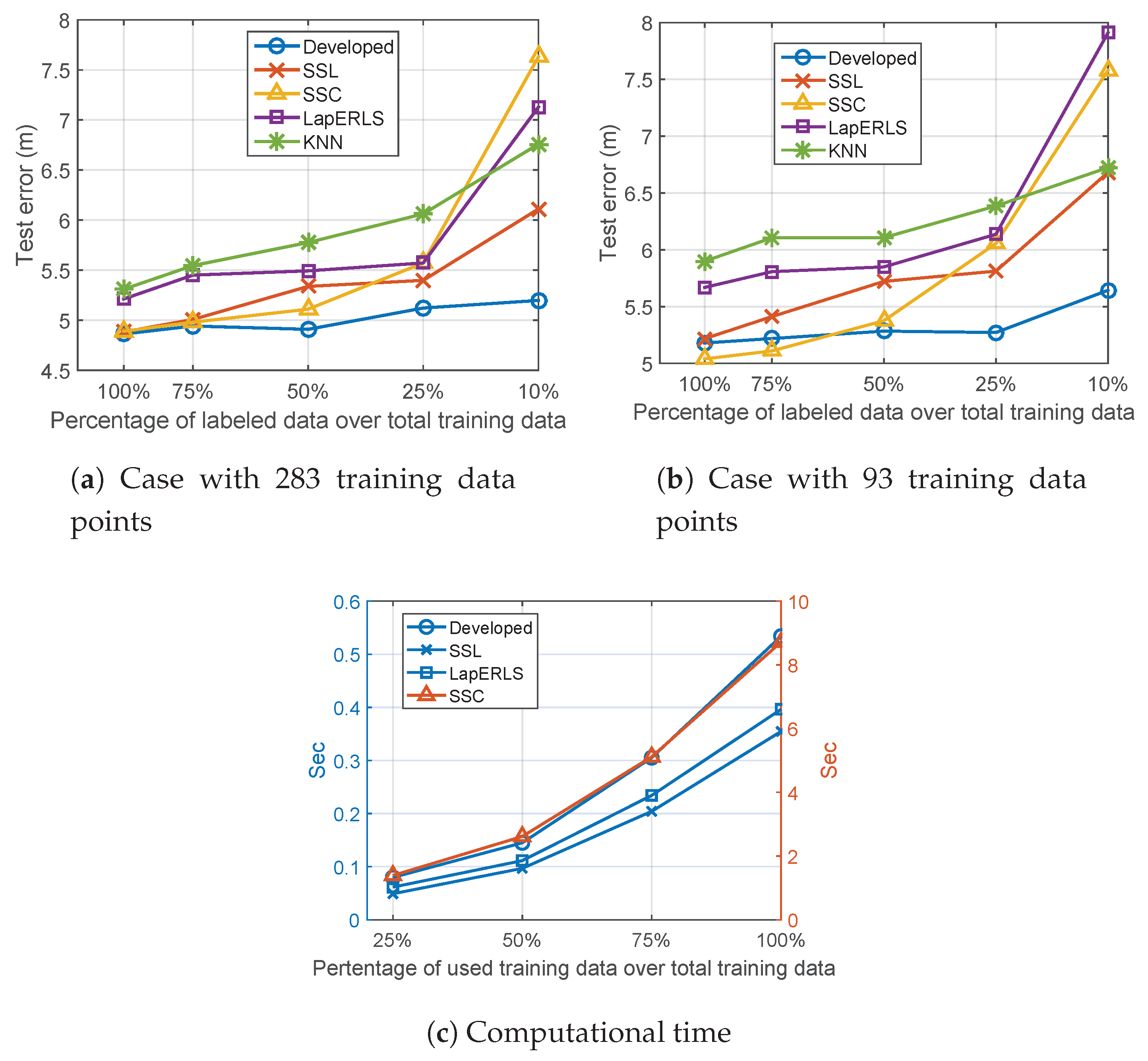
In this experiment, we compare all the benchmarks, that is, SSL, SSC, LapERLS, and the additional supervised k-NN algorithm. The parameters of the proposed algorithm are defined as ${\mu }_1=5$, ${\mu }_2=2$, $c=1$ in Equation (5), and the other parameters of the compared methods are selected for by best performance. For the experimental study, we vary the number of the used labeled training data points out of the fixed total of the training data. When 283 number of additional test data points are used, and the results using 283 and 93 training data points are shown in Figure 4a,b, respectively. From the results shown in both parts of this figure, we observe that our algorithm outperforms the compared methods. In the cases of 100% and 75% labeled data in Figure 4b, SSC provides a slightly smaller error than the other methods. However, considering the advantage given to SSC, that is, as it knows the locations of the Wi-Fi APs, this result is not noteworthy. The major contribution of our algorithm can be seen in the case where a very small number of labeled data points are used. From Figure 4a,b, our algorithm shows a slightly increasing error as fewer labeled data points are used, whereas the others exhibit a substantially increasing error when comparing the case with 25% labeled data to that with 10% case.

Finally, Figure 4c shows the CPU running time of the compared algorithms with respect to the percentage of labeled data. SSC requires more computational time than the other methods. The proposed algorithm needs slightly more time than LapERLS and SSL (an additional 0.2 s at most), due to the additional time-series term to be solved in the optimization process.

5.2. Floor Classification and Landmark Detection

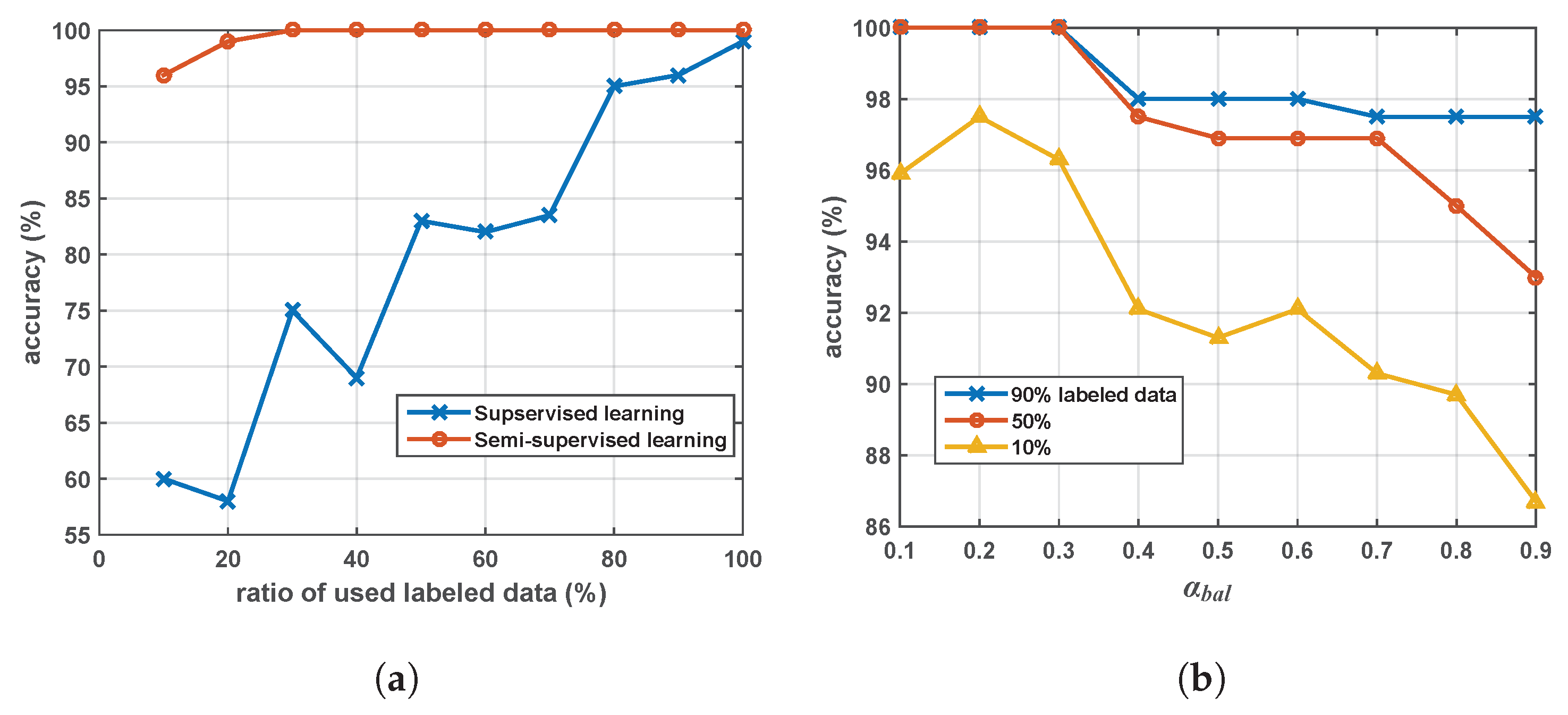
For the feature extraction, the dimensionality of the Wi-Fi RSSI set is reduced from 193 to 10, i.e., $d=193$ and $r=10$. All the RSSI values are scaled into the range [0, 1]. Figure 5a compares FDA (supervised) to the semisupervised discriminant analysis for floor level estimation. Note that because PCA is an unsupervised method, the PCA alone cannot be used for the supervised floor and landmark detections. To estimate the floor level, the k-NN method with $k=1$ is employed. In Figure 5a, the ratio of the used labeled data varies from 10% to 100%. The developed algorithm provides better accuracy than FDA. The most noticeable result appears when the ratio of the labeled data is small. Although 10% of the data is labeled, semisupervised analysis achieves 95% accuracy whereas supervised analysis results in 60% accuracy.

Selecting a tuning the balancing parameter in Equation (33) depends on a cross validation. The optimal value is selected by minimizing the training error. In Figure 5b, the floor estimation accuracy is shown with respect to the variation of parameter values ${\alpha }_{bal}$ introduced in Equation (33) and the ratio of the labeled training data. Setting a relatively large ${\alpha }_{bal}$ value intends to focus more on FDA than on PCA in the semisupervised learning analysis. In this study, ${\alpha }_{bal}=0.2$ is used in the rest of all experiments.

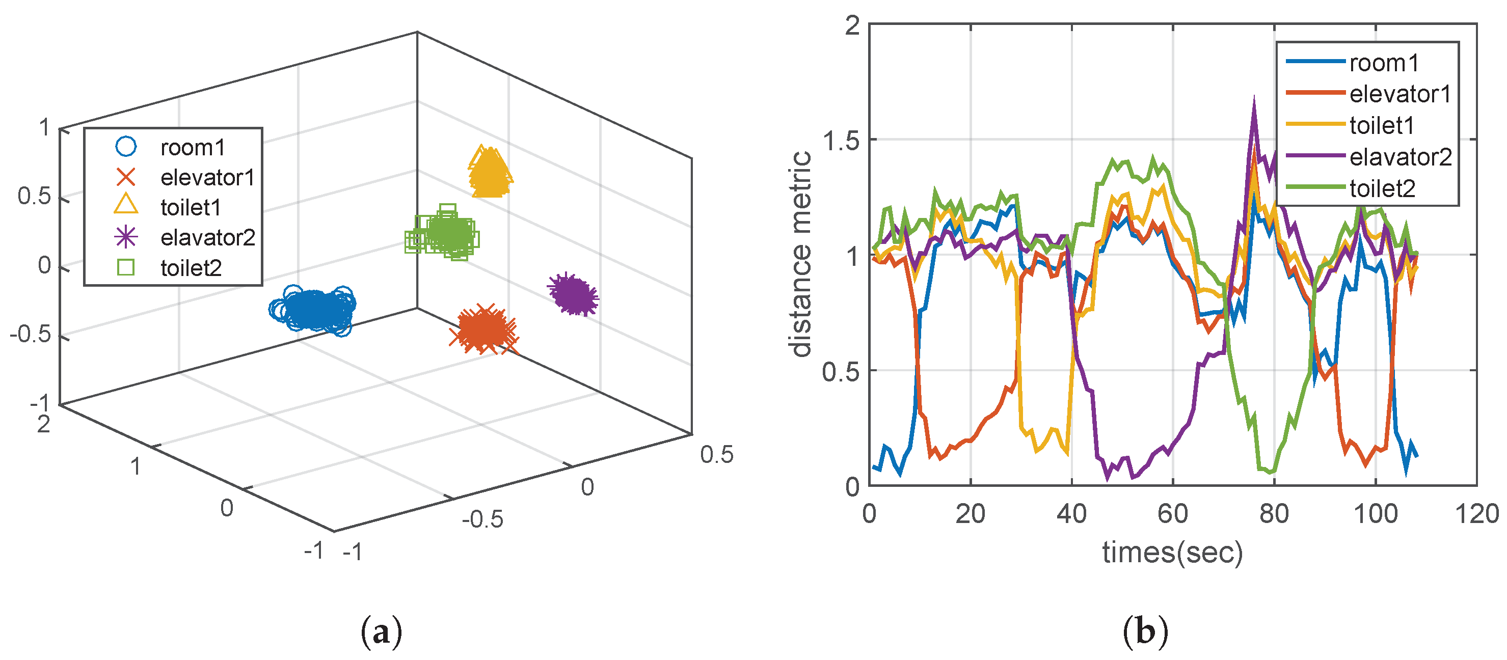
Landmarks in an indoor environment, such as toilets, elevators, and rooms, create a particular pattern of Wi-Fi RSSI measurement sets so that their distinct features can be distinctly extracted. Figure 6a clarifies the extracted features at some landmarks using the semisupervised discriminant analysis algorithm. Figure 6b shows the distance on the signal space according to a user’s path. The proposed algorithm detects the moment when the user arrives at each pre-defined landmark site with the threshold 0.3 in Figure 6b. Consequently, we can apply the landmark detection algorithm to calibrate any user’s trajectory, by determining the start and end positions. Note that these trimmed trajectories are used for the trajectory learning in Section 4.

5.3. Trajectory Learning

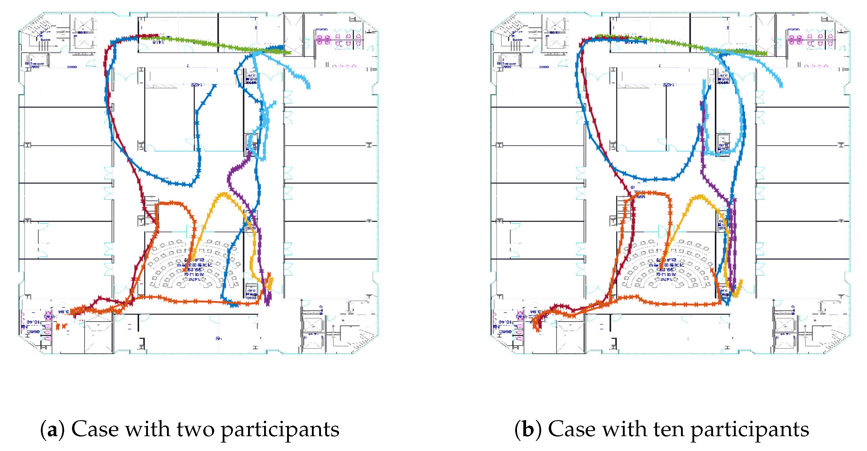
Given the trajectory samples obtained from the landmark detection, Figure 7 shows the learned map on a floor with respect to the number of the participants. In Figure 7, seven different trajectories having different start and end landmarks are drawn with the different colors. We can observe that some learned trajectories are still inaccurate in Figure 7a, as they do not match the area on the true map when only two participants join. In Figure 7b, the more participants join in, the closer the learned map approaches the ground truth.

5.4. Localization

To confirm the positioning error, two localization cases are compared with 50 number of particles setup for executing the particle filter. Figure 8a,b contains the localization results when using the learned trajectories as the prior for the particle filter. Figure 8c,d contains the localization results without using the learned trajectories. Because the user is moving, it is unable to measure the ground truths of the user’s path all the time. Instead, some waypoints are designated to alarm the user to record its location with time stamps. Based on these waypoints, the average error is calculated. Ten positioning experiments by ten different users for each case are implemented. The average error of the developed algorithm is 2.2 m. By contrast, the average error for the localization without the learned trajectories is 3.4 m. In the worst case, the proposed algorithm has 2.8 m error and the benchmark one has 5.1 m. In the best case, each has 1.3 m and 2.5 m error, respectively. Thus, the map learning improves the localization accuracy by 1.2 m on average. It is noted that in Figure 8c the positioning is remarkably inaccurate because of the indoor environment composing majority of open space, whereas the localization on the aisles are relatively more precise. On the other hand, as shown in Figure 8a, the accurately learned map information supports to overcome this environmental restriction by enhancing the accuracy. The last remark of the experimental result analysis between Figure 8b,d is the positioning regarding the south room. Because the true map information is not given in this paper, it is unable for the localization in Figure 8d to recognize the wall between the room and aisle. On the other hand, due to aid of the trajectory learning, the proposed method recognizes the isolation by the wall, in which Figure 8b shows the clear–separate position estimations between the room and the aisle.

6. Conclusions

In this study, we investigated indoor localization performing simultaneous floor classification, landmark detection, positioning, and map learning. The study was divided into three topics: (i) feature extraction from Wi-Fi RSSIs for floor classification and landmark detection, (ii) mobile fingerprinting and pseudolabeling for positioning, and (iii) mapless localization.

In the first part, characteristics of Wi-Fi RSSIs were determined by pattern recognition, using a semisupervised discriminant analysis. The proposed algorithm extracted the features from the noisy Wi-Fi signal data by reducing them from a high to a low dimension. During this process, worthless elements were removed to obtain clustered data points according to the different floors and different landmarks. At the same time, by investigating the distance between a test point and the training data on the reduced signal space, we successfully detected the floor and landmark changes.

The second part addressed the efficiency of fingerprinting. Compared to conventional static fingerprinting, our algorithm improved the efficiency for collecting the training data because a user could be mobile during the collection without manually labelling the position at every grid point in the area of interest. The proposed pseudolabeling algorithm based on the semisupervised regression aimed to obtain accurate pseudolabeled positions for the unlabeled training data. Considering both the spatial and temporal aspect, we formalized the optimization based on a graph Laplacian and H–P filter. Further, the optimization provided a closed-form solution, which enabled fast computation.

In the last part, we considered the situation where the true map information is not available. The key idea was crowdsourcing, from which we can obtain trajectory samples. From the experimental results, as more participants joined in, the learned map was updated more accurately. The experiments conducted in this study involved floors in a multifloor office building. Many people participated in validating our algorithm. The integration of all the parts led to accurate localization.